
Evaluation of the Plant Phenology Index (PPI), NDVI and EVI for Start-of-Season Trend Analysis of the Northern Hemisphere Boreal Zone


Abstract
:
1. Introduction
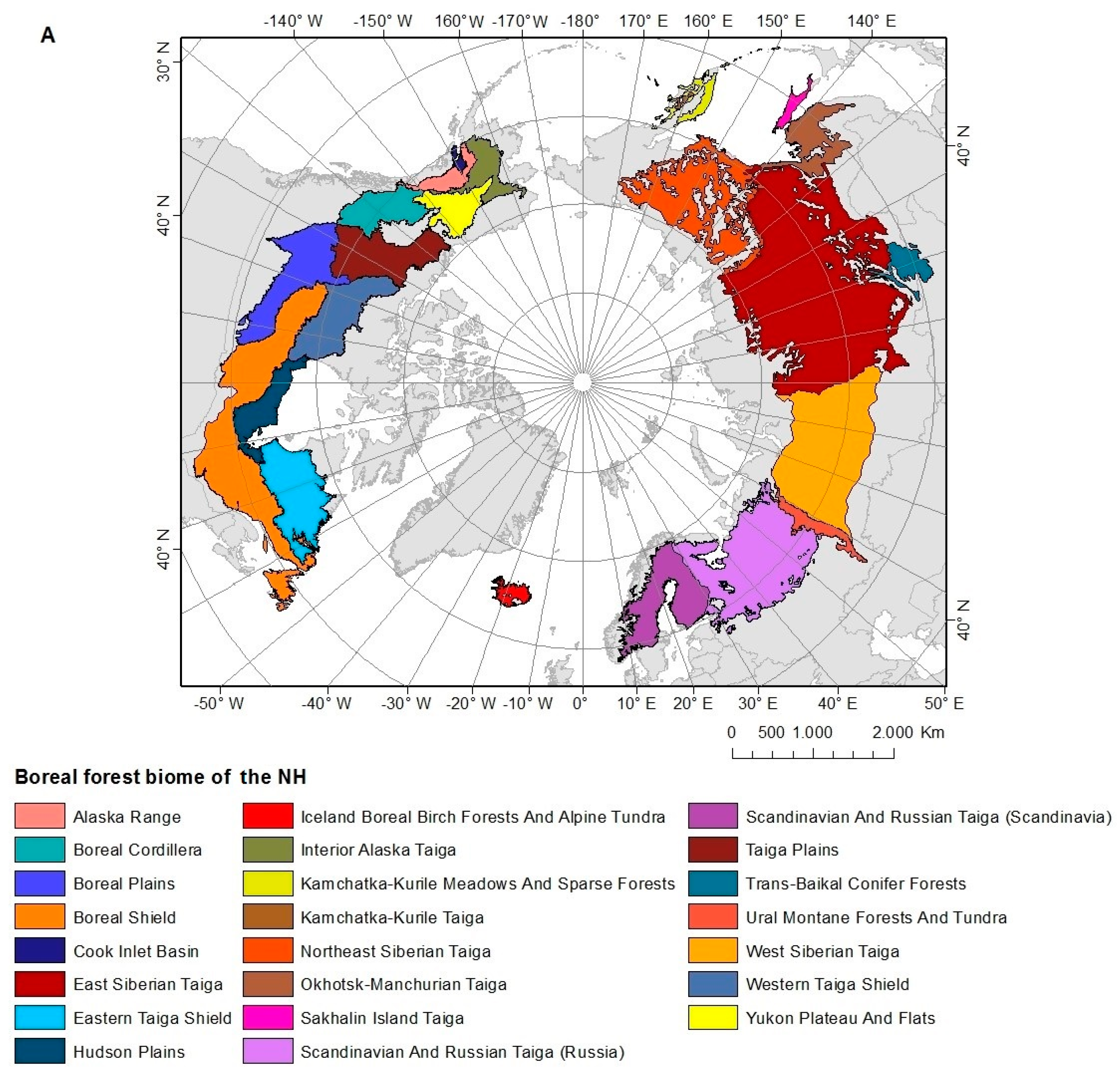
2. Study Area
3. Materials and Methods
3.1. Satellite Data
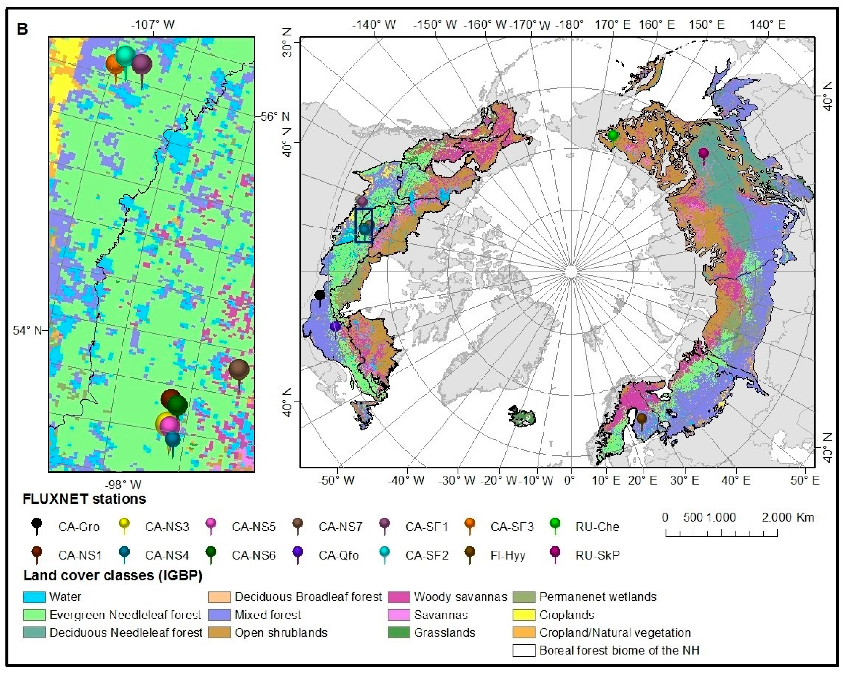
3.2. Flux Tower Data
3.3. Vegetation Indices
- M—a maximum difference between NIR and red MODIS NBAR was calculated for each pixel, for the time period 2000–2014.
- DVI value was set to 0.09, which is an empirically defined value [36]. DVIs can cause negative values if canopy DVI is lower than , which can occur during snowy conditions or for an ecosystem with very bright soil. The empirical value of was still considered to be applicable in this study, since negative estimates will not alter linearity between PPI and LAI [36].
- zenith angle (θ) value for each pixel location was acquired from “Zenith Angle at local solar noon” data layer in the MCD43C4 products.
- G value was set to 0.5 based on [59] who found that for a spherical needle (leaf) orientation G is 0.5, regardless of directions of the solar beam (different view directions). According to [36], G 0.5 is also valid for a flat leaf, when assuming a spherical (uniform) leaf angle distribution and may therefore be used in the calculation of PPI.
3.4. Start of Season (SOS) Retrieval
3.5. Statistical Analysis
4. Results
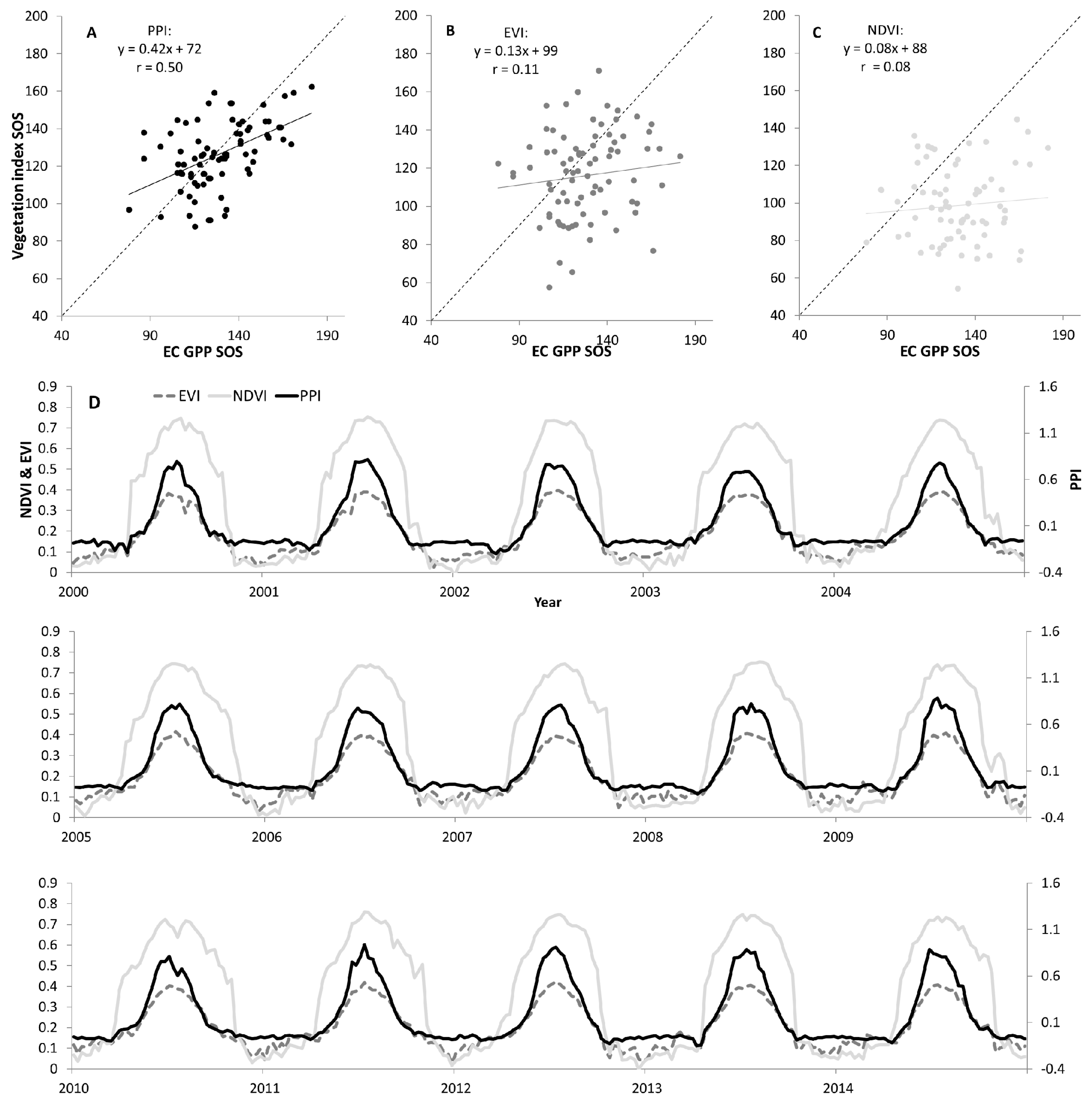
4.1. Evaluation of VI-Based SOS against in Situ GPP-Based SOS
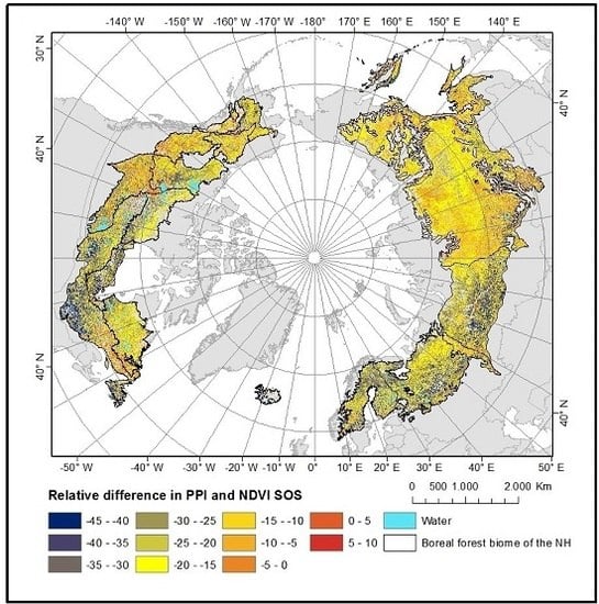
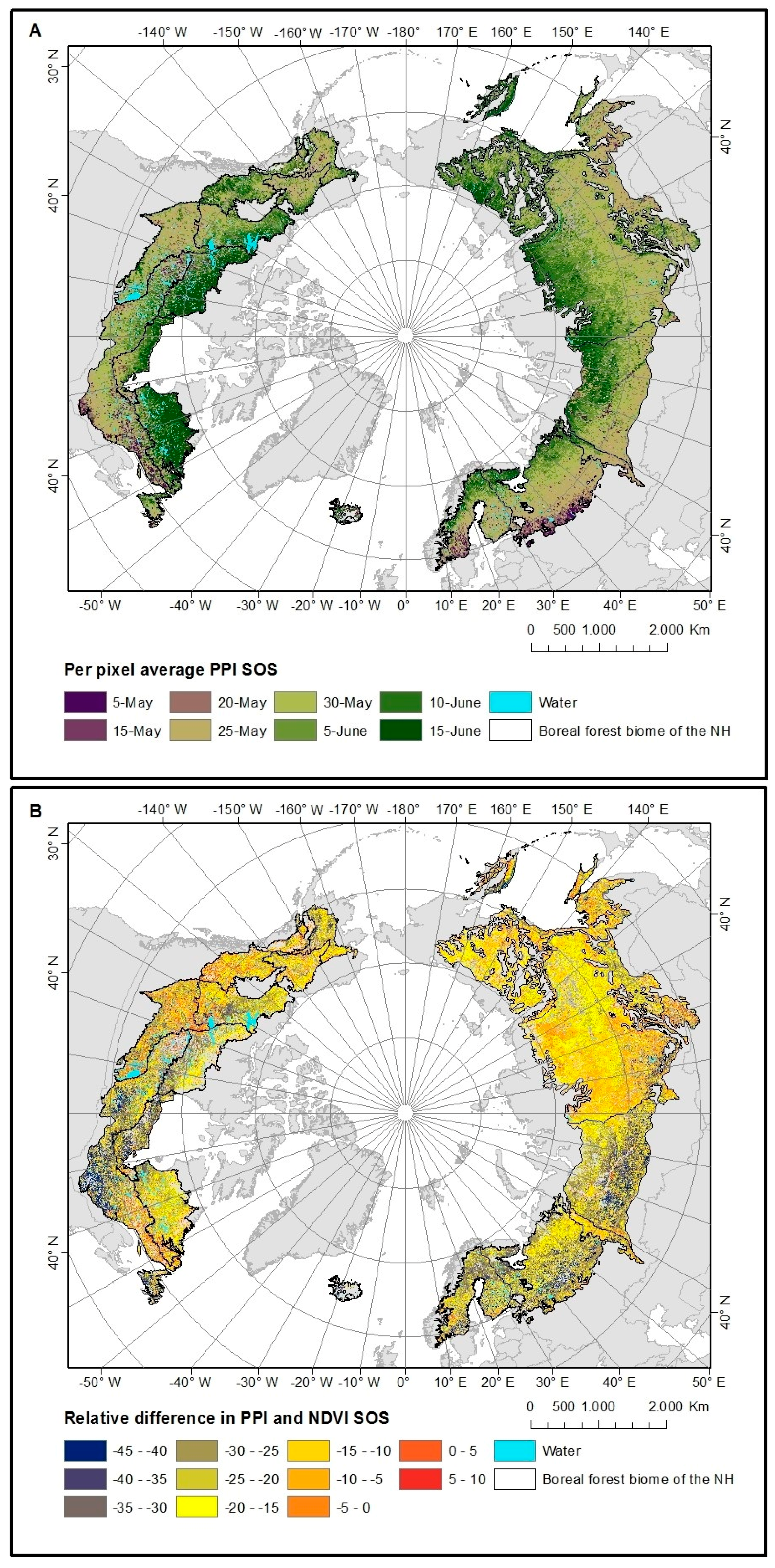
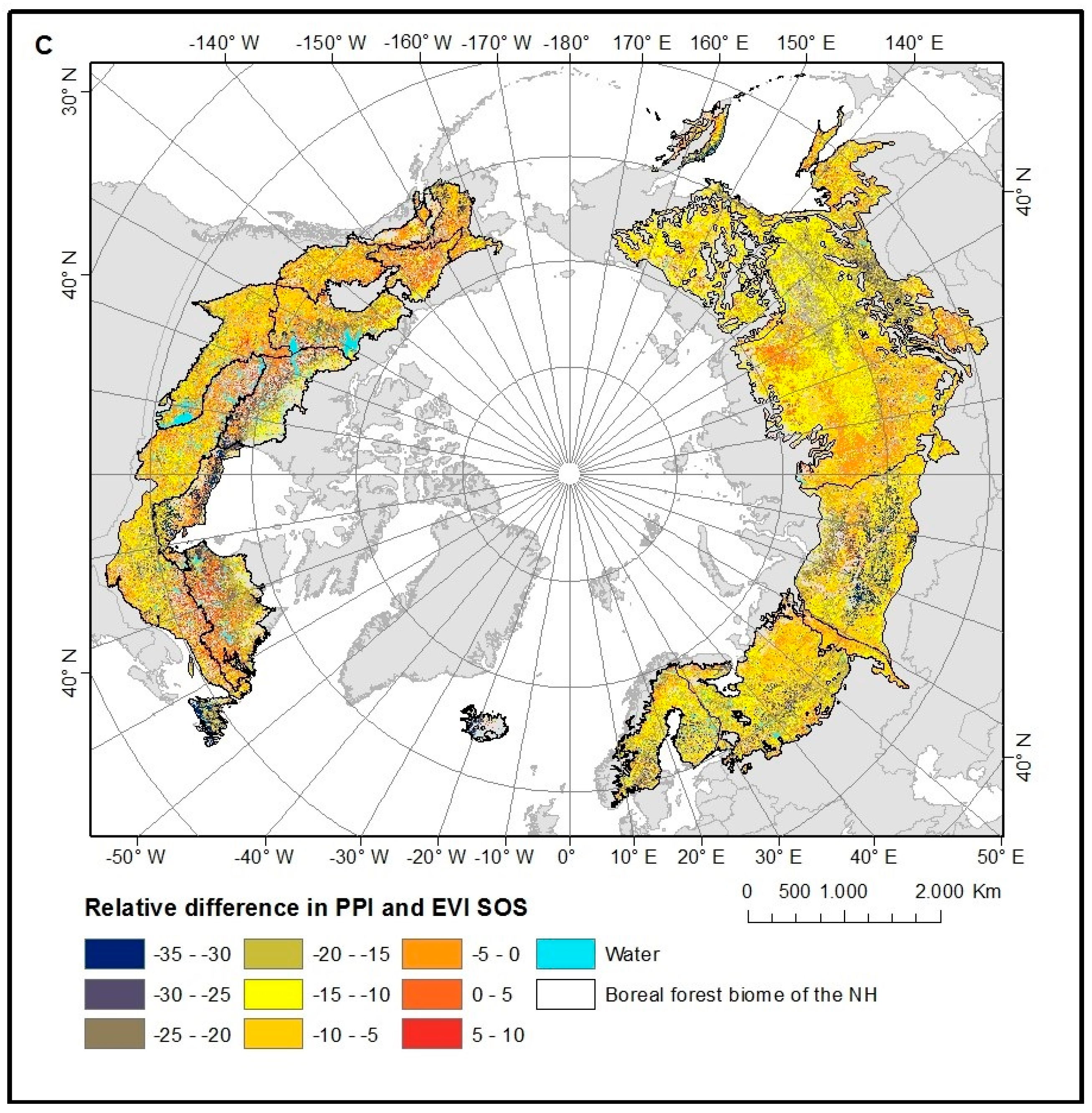
4.2. Spatial Patterns of VI SOS Estimates
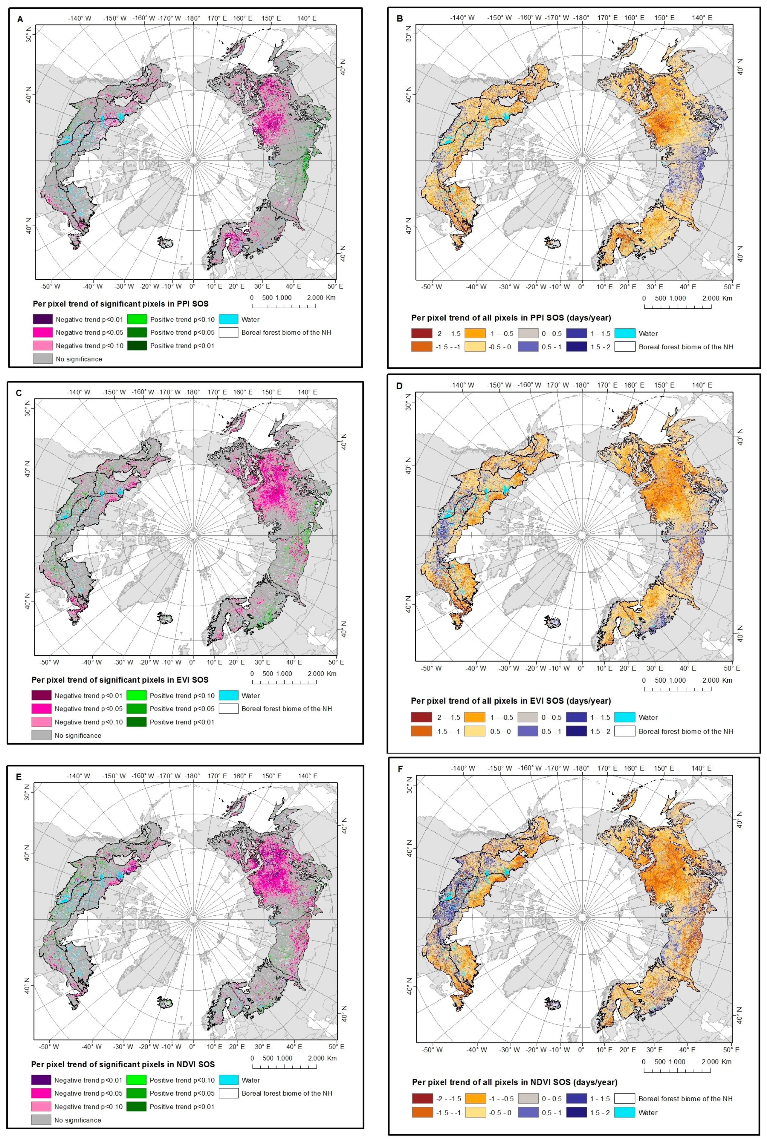
4.3. Trends in VI SOS Estimates
4.3.1. PPI
4.3.2. EVI and NDVI
5. Discussion
5.1. VI SOS Detection and Evaluation against GPP-SOS
5.2. VI SOS Spatial Patterns
5.3. VI SOS Temporal Patterns
6. Conclusions
Supplementary Materials
Acknowledgments
Author Contributions
Conflicts of Interest
Appendix A

| Site ID: Site Name | Temporal Data Availability | Location (Lat; Long) | IGBP Vegetation Cover |
|---|---|---|---|
| FI-Hyy: Hyytiala | 2000–2014 | 61.8475; | Evergreen needleleaf (ENF) |
| 24.2950 | |||
| RU-SkP: Spasskaya Pad larch | 2012–2014 | 62.2550; | Deciduous needleleaf (DNF) |
| 129.1680 | |||
| RU-Che: Cherskii | 2002–2005 | 68.6130; | Permanent wetlands (WET) |
| 161.3414 | |||
| CA-Qfo: Quebec-Eastern Boreal, Mature Black Spruce | 2003–2010 | 49.6925; | Evergreen needleleaf (ENF) |
| −74.3421 | |||
| CA-Gro: Ontario-Groundhog River, Boreal mixed wood Forest | 2003–2014 | 48.2167; | Mixed Forest (MF) |
| −82.1556 | |||
| CA-NS1: UCI-1850 burn site | 2002–2005 | 55.8792; | Evergreen needleleaf (ENF) |
| −98.4839 | |||
| CA-NS3:UCI-1964 burn site | 2001–2005 | 55.9117; | Evergreen needleleaf (ENF) |
| −98.3822 | |||
| CA-NS4: UCI-1964 burn site wet | 2002–2005 | 55.9117; | Evergreen needleleaf (ENF) |
| −98.3822 | |||
| CA-NS5: UCI-1964 burn site | 2001–2005 | 55.8631; | Evergreen needleleaf (ENF) |
| −98.4850 | |||
| CA-NS6: UCI-1998 burn site | 2001–2005 | 55.9167; | Open shrublands (OSH) |
| −98.9644 | |||
| CA-NS7:UCI-1998 burn site | 2002–2005 | 56.6358; | Open shrublands (OSH) |
| −99.9483 | |||
| CA-SF1: Saskatchewan-Western Boreal | 2001–2006 | 54.4850; | Evergreen needleleaf (ENF) |
| −105.8176 | |||
| CA-SF2: Saskatchewan-Western Boreal | 2001–2005 | 54.2539; | Evergreen needleleaf (ENF) |
| −105.8775 | |||
| CA-SF3: Saskatchewan-Western Boreal, forest burned in 1998 | 2001–2006 | 54.0916; | Open shrublands (OSH) |
| −106.0053 |
References
- Piao, S.L.; Tan, J.G.; Chen, A.P.; Fu, Y.H.; Ciais, P.; Liu, Q.; Janssens, I.A.; Vicca, S.; Zeng, Z.Z.; Jeong, S.J.; et al. Leaf onset in the Northern Hemisphere triggered by daytime temperature. Nat. Commun. 2015, 6. [Google Scholar] [CrossRef] [PubMed]
- Walther, G.R.; Post, E.; Convey, P.; Menzel, A.; Parmesan, C.; Beebee, T.J.C.; Fromentin, J.M.; Hoegh-Guldberg, O.; Bairlein, F. Ecological responses to recent climate change. Nature 2002, 416, 389–395. [Google Scholar] [CrossRef] [PubMed]
- Penuelas, J.; Filella, I. Phenology—Responses to a warming world. Science 2001, 294, 793–795. [Google Scholar] [CrossRef] [PubMed]
- Nemani, R.R.; Keeling, C.D.; Hashimoto, H.; Jolly, W.M.; Piper, S.C.; Tucker, C.J.; Myneni, R.B.; Running, S.W. Climate-driven increases in global terrestrial net primary production from 1982 to 1999. Science 2003, 300, 1560–1563. [Google Scholar] [CrossRef] [PubMed]
- Piao, S.L.; Friedlingstein, P.; Ciais, P.; Zhou, L.M.; Chen, A.P. Effect of climate and CO2 changes on the greening of the Northern Hemisphere over the past two decades. Geophys. Res. Lett. 2006, 33. [Google Scholar] [CrossRef]
- Cleland, E.E.; Chuine, I.; Menzel, A.; Mooney, H.A.; Schwartz, M.D. Shifting plant phenology in response to global change. Trends Ecol. Evol. 2007, 22, 357–365. [Google Scholar] [CrossRef] [PubMed]
- Zeng, H.Q.; Jia, G.S.; Epstein, H. Recent changes in phenology over the northern high latitudes detected from multi-satellite data. Environ. Res. Lett. 2011, 6. [Google Scholar] [CrossRef]
- Stockli, R.; Vidale, P.L. European plant phenology and climate as seen in a 20-year AVHRR land-surface parameter dataset. Int. J. Remote. Sens. 2004, 25, 3303–3330. [Google Scholar] [CrossRef]
- Penuelas, J.; Rutishauser, T.; Filella, I. Phenology feedbacks on climate change. Science 2009, 324, 887–888. [Google Scholar] [CrossRef] [PubMed]
- Liu, Q.; Fu, Y.S.H.; Zeng, Z.Z.; Huang, M.T.; Li, X.R.; Piao, S.L. Temperature, precipitation, and insolation effects on autumn vegetation phenology in temperate China. Glob. Chang. Biol. 2016, 22, 644–655. [Google Scholar] [CrossRef] [PubMed]
- Badeck, F.W.; Bondeau, A.; Bottcher, K.; Doktor, D.; Lucht, W.; Schaber, J.; Sitch, S. Responses of spring phenology to climate change. New Phytol. 2004, 162, 295–309. [Google Scholar] [CrossRef]
- Wang, X.H.; Piao, S.L.; Ciais, P.; Li, J.S.; Friedlingstein, P.; Koven, C.; Chen, A.P. Spring temperature change and its implication in the change of vegetation growth in North America from 1982 to 2006. Porc. Natl. Acad. Sci. USA 2011, 108, 1240–1245. [Google Scholar] [CrossRef] [PubMed]
- Piao, S.L.; Nan, H.J.; Huntingford, C.; Ciais, P.; Friedlingstein, P.; Sitch, S.; Peng, S.S.; Ahlstrom, A.; Canadell, J.G.; Cong, N.; et al. Evidence for a weakening relationship between interannual temperature variability and northern vegetation activity. Nat. Commun. 2014, 5. [Google Scholar] [CrossRef] [PubMed]
- Peng, S.S.; Piao, S.L.; Ciais, P.; Myneni, R.B.; Chen, A.P.; Chevallier, F.; Dolman, A.J.; Janssens, I.A.; Penuelas, J.; Zhang, G.X.; et al. Asymmetric effects of daytime and night-time warming on Northern Hemisphere vegetation. Nature 2013, 501, 88–92. [Google Scholar] [CrossRef] [PubMed]
- Melaas, E.K.; Richardson, A.D.; Friedl, M.A.; Dragoni, D.; Gough, C.M.; Herbst, M.; Montagnani, L.; Moors, E. Using fluxnet data to improve models of springtime vegetation activity onset in forest ecosystems. Agric. For. Meteorol. 2013, 171, 46–56. [Google Scholar] [CrossRef]
- Barichivich, J.; Briffa, K.R.; Myneni, R.B.; Osborn, T.J.; Melvin, T.M.; Ciais, P.; Piao, S.L.; Tucker, C. Large-scale variations in the vegetation growing season and annual cycle of atmospheric CO2 at high northern latitudes from 1950 to 2011. Glob. Chang. Biol. 2013, 19, 3167–3183. [Google Scholar] [CrossRef] [PubMed]
- Myneni, R.B.; Dong, J.; Tucker, C.J.; Kaufmann, R.K.; Kauppi, P.E.; Liski, J.; Zhou, L.; Alexeyev, V.; Hughes, M.K. A large carbon sink in the woody biomass of northern forests. Proc. Natl. Acad. Sci. USA 2001, 98, 14784–14789. [Google Scholar] [CrossRef] [PubMed]
- Randerson, J.T.; Field, C.B.; Fung, I.Y.; Tans, P.P. Increases in early season ecosystem uptake explain recent changes in the seasonal cycle of atmospheric CO2 at high northern latitudes. Geophys. Res. Lett. 1999, 26, 2765–2768. [Google Scholar] [CrossRef]
- Davi, H.; Dufrene, E.; Francois, C.; Le Maire, G.; Loustau, D.; Bosc, A.; Rambal, S.; Granier, A.; Moors, E. Sensitivity of water and carbon fluxes to climate changes from 1960 to 2100 in European forest ecosystems. Agric. For. Meteorol. 2006, 141, 35–56. [Google Scholar] [CrossRef]
- Myneni, R.B.; Keeling, C.D.; Tucker, C.J.; Asrar, G.; Nemani, R.R. Increased plant growth in the northern high latitudes from 1981 to 1991. Nature 1997, 386, 698–702. [Google Scholar] [CrossRef]
- Pan, Y.D.; Birdsey, R.A.; Fang, J.Y.; Houghton, R.; Kauppi, P.E.; Kurz, W.A.; Phillips, O.L.; Shvidenko, A.; Lewis, S.L.; Canadell, J.G.; et al. A large and persistent carbon sink in the world’s forests. Science 2011, 333, 988–993. [Google Scholar] [CrossRef] [PubMed]
- Deluca, T.H.; Boisvenue, C. Boreal forest soil carbon: Distribution, function and modelling. Forestry 2012, 85, 161–184. [Google Scholar] [CrossRef]
- Zhao, J.J.; Zhang, H.Y.; Zhang, Z.X.; Guo, X.Y.; Li, X.D.; Chen, C. Spatial and temporal changes in vegetation phenology at middle and high latitudes of the Northern Hemisphere over the past three decades. Remote Sens. 2015, 7, 10973–10995. [Google Scholar] [CrossRef]
- Jeong, S.J.; Ho, C.H.; Gim, H.J.; Brown, M.E. Phenology shifts at start vs. End of growing season in temperate vegetation over the Northern Hemisphere for the period 1982–2008. Glob. Chang. Biol. 2011, 17, 2385–2399. [Google Scholar] [CrossRef]
- Garonna, I.; De Jong, R.; De Wit, A.J.W.; Mucher, C.A.; Schmid, B.; Schaepman, M.E. Strong contribution of autumn phenology to changes in satellite-derived growing season length estimates across Europe (1982–2011). Glob. Chang. Biol. 2014, 20, 3457–3470. [Google Scholar] [CrossRef] [PubMed]
- Maignan, F.; Breon, F.M.; Bacour, C.; Demarty, J.; Poirson, A. Interannual vegetation phenology estimates from global AVHRR measurements—Comparison with in situ data and applications. Remote Sens. Environ. 2008, 112, 496–505. [Google Scholar] [CrossRef]
- Delbart, N.; Le Toan, T.; Kergoat, L.; Fedotova, V. Remote sensing of spring phenology in boreal regions: A free of snow-effect method using NOAA-AVHRR and SPOT-VGT data (1982–2004). Remote Sens. Environ. 2006, 101, 52–62. [Google Scholar] [CrossRef]
- Park, T.; Ganguly, S.; Tommervik, H.; Euskirchen, E.S.; Hogda, K.A.; Karlsen, S.R.; Brovkin, V.; Nemani, R.R.; Myneni, R.B. Changes in growing season duration and productivity of northern vegetation inferred from long-term remote sensing data. Environ. Res. Lett. 2016, 11. [Google Scholar] [CrossRef]
- Tucker, C.J. Red and photographic infrared linear combinations for monitoring vegetation. Remote Sens. Environ. 1979, 8, 127–150. [Google Scholar] [CrossRef]
- Rouse, J.W.; Haas, R.H.; Schell, J.A.; Deering, D.W.; Harlan, J.C. Monitoring the Vernal Advancement of Retrogradation of Natural Vegetation; Type III, Final Report; NASA/GSFC: Greenbelt, MD, USA, 1974.
- Wang, Z.; Liu, C.; Huete, A. From AVHRR-NDVI to MODIS-EVI: Advances in vegetation index research. Acta Ecol. Sin. 2002, 23, 979–987. [Google Scholar]
- Huete, A.R. A soil-adjusted vegetation index (SAVI). Remote Sens. Environ. 1988, 25, 295–309. [Google Scholar] [CrossRef]
- Huete, A.; Didan, K.; Miura, T.; Rodriguez, E.P.; Gao, X.; Ferreira, L.G. Overview of the radiometric and biophysical performance of the MODIS vegetation indices. Remote Sens. Environ. 2002, 83, 195–213. [Google Scholar] [CrossRef]
- Wang, X.H.; Piao, S.L.; Xu, X.T.; Ciais, P.; MacBean, N.; Myneni, R.B.; Li, L. Has the advancing onset of spring vegetation green-up slowed down or changed abruptly over the last three decades? Glob. Ecol. Biogeogr. 2015, 24, 621–631. [Google Scholar] [CrossRef]
- White, M.A.; de Beurs, K.M.; Didan, K.; Inouye, D.W.; Richardson, A.D.; Jensen, O.P.; O’Keefe, J.; Zhang, G.; Nemani, R.R.; van Leeuwen, W.J.D.; et al. Intercomparison, interpretation, and assessment of spring phenology in North America estimated from remote sensing for 1982–2006. Glob. Chang. Biol. 2009, 15, 2335–2359. [Google Scholar] [CrossRef]
- Jin, H.X.; Eklundh, L. A physically based vegetation index for improved monitoring of plant phenology. Remote Sens. Environ. 2014, 152, 512–525. [Google Scholar] [CrossRef]
- Jönsson, A.M.; Eklundh, L.; Hellström, M.; Bärring, L.; Jönsson, P. Annual changes in MODIS vegetation indices of Swedish coniferous forests in relation to snow dynamics and tree phenology. Remote Sens. Environ. 2010, 114, 2719–2730. [Google Scholar] [CrossRef]
- Parmesan, C.; Yohe, G. A globally coherent fingerprint of climate change impacts across natural systems. Nature 2003, 421, 37–42. [Google Scholar] [CrossRef] [PubMed]
- Fu, Y.S.H.; Piao, S.L.; Op de Beeck, M.; Cong, N.; Zhao, H.F.; Zhang, Y.; Menzel, A.; Janssens, I.A. Recent spring phenology shifts in western central Europe based on multiscale observations. Glob. Ecol. Biogeogr. 2014, 23, 1255–1263. [Google Scholar] [CrossRef]
- Hassan, Q.K.; Rahman, K.M. Applicability of remote sensing-based surface temperature regimes in determining deciduous phenology over boreal forest. J. Plant Ecol. 2013, 6, 84–91. [Google Scholar] [CrossRef]
- Delbart, N.; Kergoat, L.; Le Toan, T.; Lhermitte, J.; Picard, G. Determination of phenological dates in boreal regions using Normalized Difference Water Index. Remote Sens. Environ. 2005, 97, 26–38. [Google Scholar] [CrossRef]
- Sekhon, N.S.; Hassan, Q.K.; Sleep, R.W. Evaluating potential of MODIS-based indices in determining “snow gone” stage over forest-dominant regions. Remote Sens. 2010, 2, 1348–1363. [Google Scholar] [CrossRef]
- Walther, S.; Voigt, M.; Thum, T.; Gonsamo, A.; Zhang, Y.; Köhler, P.; Jung, M.; Varlagin, A.; Guanter, L. Satellite chlorophyll fluorescence measurements reveal large-scale decoupling of photosynthesis and greenness dynamics in boreal evergreen forests. Glob. Chang. Biol. 2016, 22, 2979–2996. [Google Scholar] [CrossRef] [PubMed]
- Wu, C.Y.; Gonsamo, A.; Gough, C.M.; Chen, J.M.; Xu, S.G. Modeling growing season phenology in North American forests using seasonal mean vegetation indices from MODIS. Remote Sens. Environ. 2014, 147, 79–88. [Google Scholar] [CrossRef]
- Guyon, D.; Guillot, M.; Vitasse, Y.; Cardot, H.; Hagolle, O.; Delzon, S.; Wigneron, J.P. Monitoring elevation variations in leaf phenology of deciduous broadleaf forests from spot/vegetation time-series. Remote Sens. Environ. 2011, 115, 615–627. [Google Scholar] [CrossRef]
- Hufkens, K.; Friedl, M.A.; Keenan, T.F.; Sonnentag, O.; Bailey, A.; O’Keefe, J.; Richardson, A.D. Ecological impacts of a widespread frost event following early spring leaf-out. Glob. Chang. Biol. 2012, 18, 2365–2377. [Google Scholar] [CrossRef]
- Hmimina, G.; Dufrene, E.; Pontailler, J.Y.; Delpierre, N.; Aubinet, M.; Caquet, B.; de Grandcourt, A.; Burban, B.; Flechard, C.; Granier, A.; et al. Evaluation of the potential of MODIS satellite data to predict vegetation phenology in different biomes: An investigation using ground-based NDVI measurements. Remote Sens. Environ. 2013, 132, 145–158. [Google Scholar] [CrossRef]
- Jin, H. Remote Sensing Phenology at European Northern Latitudes—From Ground Spectral Towers to Satellites; Department of Physical Geography and Ecosystem Science, Lund University: Lund, Sweden, 2015. [Google Scholar]
- Richardson, A.D.; Keenan, T.F.; Migliavacca, M.; Ryu, Y.; Sonnentag, O.; Toomey, M. Climate change, phenology, and phenological control of vegetation feedbacks to the climate system. Agric. For. Meteorol. 2013, 169, 156–173. [Google Scholar] [CrossRef]
- Nagai, S.; Nasahara, K.N.; Muraoka, H.; Akiyama, T.; Tsuchida, S. Field experiments to test the use of the Normalized-Difference Vegetation Index for phenology detection. Agric. For. Meteorol. 2010, 150, 152–160. [Google Scholar] [CrossRef]
- Olson, D.M.; Dinerstein, E.; Wikramanayake, E.D.; Burgess, N.D.; Powell, G.V.N.; Underwood, E.C.; D’Amico, J.A.; Itoua, I.; Strand, H.E.; Morrison, J.C.; et al. Terrestrial ecoregions of the worlds: A new map of life on earth. Bioscience 2001, 51, 933–938. [Google Scholar] [CrossRef]
- De Beurs, K.M.; Henebry, G.M. A land surface phenology assessment of the northern polar regions using MODIS reflectance time series. Can. J. Remote Sens. 2010, 36, S87–S110. [Google Scholar] [CrossRef]
- Riseborough, D.; Shiklomanov, N.; Etzelmuller, B.; Gruber, S.; Marchenko, S. Recent advances in permafrost modelling. Permafr. Periglac. 2008, 19, 137–156. [Google Scholar] [CrossRef]
- Schaaf, C.B.; Gao, F.; Strahler, A.H.; Lucht, W.; Li, X.W.; Tsang, T.; Strugnell, N.C.; Zhang, X.Y.; Jin, Y.F.; Muller, J.P.; et al. First operational BRDF, albedo NADIR reflectance products from MODIS. Remote Sens. Environ. 2002, 83, 135–148. [Google Scholar] [CrossRef]
- Hansen, M.C.; Potapov, P.V.; Moore, R.; Hancher, M.; Turubanova, S.A.; Tyukavina, A.; Thau, D.; Stehman, S.V.; Goetz, S.J.; Loveland, T.R.; et al. High-resolution global maps of 21st-century forest cover change. Science 2013, 342, 850–853. [Google Scholar] [CrossRef] [PubMed]
- Roujean, J.L.; Leroy, M.; Deschamps, P.Y. A bidirectional reflectance model of the earths surface for the correction of remote-sensing data. J. Geophys. Res. Atmos. 1992, 97, 20455–20468. [Google Scholar] [CrossRef]
- Suehrcke, H.; Mccormick, P.G. The diffuse fraction of instantaneous solar-radiation. Sol. Energy 1988, 40, 423–430. [Google Scholar] [CrossRef]
- Kasten, F.; Young, A.T. Revised optical air-mass tables and approximation formula. Appl. Opt. 1989, 28, 4735–4738. [Google Scholar] [CrossRef] [PubMed]
- Stenberg, P. A note on the G-function for needle leaf canopies. Agric. For. Meteorol. 2006, 136, 76–79. [Google Scholar] [CrossRef]
- Jonsson, P.; Eklundh, L. TIMESAT—A program for analyzing time-series of satellite sensor data. Comput. Geosci. 2004, 30, 833–845. [Google Scholar] [CrossRef]
- Beck, P.S.A.; Atzberger, C.; Hogda, K.A.; Johansen, B.; Skidmore, A.K. Improved monitoring of vegetation dynamics at very high latitudes: A new method using MODIS NDVI. Remote Sens. Environ. 2006, 100, 321–334. [Google Scholar] [CrossRef]
- Jonsson, P.; Eklundh, L. Seasonality extraction by function fitting to time-series of satellite sensor data. IEEE Trans. Geosci. Remote 2002, 40, 1824–1832. [Google Scholar] [CrossRef]
- Eklundh, L.; Jönsson, P. TIMESAT: A software package for time-series processing and assessment of vegetation dynamics. In Remote sensing Time Series: Revealing Land Surface Dynamics; Kuenzer, C., Dech, S., Wagner, W., Eds.; Springer International Publishing: Cham, Switzerland, 2015; pp. 141–158. ISBN 978-3-319-15967-6. [Google Scholar]
- Tan, B.; Morisette, J.T.; Wolfe, R.E.; Gao, F.; Ederer, G.A.; Nightingale, J.; Pedelty, J.A. An enhanced TIMESAT algorithm for estimating vegetation phenology metrics from MODIS data. IEEE J. Sel. Top. Appl. Earth Obs. Remote Sens. 2011, 4, 361–371. [Google Scholar] [CrossRef]
- Fensholt, R.; Proud, S.R. Evaluation of earth observation based global long term vegetation trends—Comparing GIMMS and MODIS global NDVI time series. Remote Sens. Environ. 2012, 119, 131–147. [Google Scholar] [CrossRef]
- Sen, P.K. Estimates of the regression coefficient based on Tendall’s Tau. J. Am. Stat. Assoc. 1968, 63, 1379–1389. [Google Scholar] [CrossRef]
- Theil, H. A Rank-Invariant Method of Linear and Polynomial Regression Analysis, I, II and III; The Royal Netherlands Academy of Science: Amsterdam, The Netherlands, 1950. [Google Scholar]
- Eastman, J.R.; Sangermano, F.; Machado, E.A.; Rogan, J.; Anyamba, A. Global trends in seasonality of Normalized Difference Vegetation Index (NDVI), 1982–2011. Remote Sens. 2013, 5, 4799–4818. [Google Scholar] [CrossRef]
- Hoaglin, D.C.; Mosteller, F.; Tukey, J.W. Understanding Robust and Exploratory Data Analysis; Wiley: New York, NY, USA, 1983. [Google Scholar]
- Zhang, X.Y.; Tan, B.; Yu, Y.Y. Interannual variations and trends in global land surface phenology derived from Enhanced Vegetation Index during 1982–2010. Int. J. Biometeorol. 2014, 58, 547–564. [Google Scholar] [CrossRef] [PubMed]
- Metsamaki, S.; Mattila, O.P.; Pulliainen, J.; Niemi, K.; Luojus, K.; Bottcher, K. An optical reflectance model-based method for fractional snow cover mapping applicable to continental scale. Remote Sens. Environ. 2012, 123, 508–521. [Google Scholar] [CrossRef]
- Wu, C.; Peng, D.; Soudani, K.; Siebicke, L.; Gough, C.M.; Arain, M.A.; Bohrer, G.; Lafleur, P.M.; Peichl, M.; Gonsamo, A.; et al. Land surface phenology derived from Normalized Difference Vegetation Index (NDVI) at global fluxnet sites. Agric. For. Meteorol. 2017, 233, 171–182. [Google Scholar] [CrossRef]
- Rodrigues, A.; Marcal, A.R.S.; Cunha, M. Monitoring vegetation dynamics inferred by satellite data using the phenosat tool. IEEE Trans. Geosci. Remote 2013, 51, 2096–2104. [Google Scholar] [CrossRef]
- White, K.; Pontius, J.; Schaberg, P. Remote sensing of spring phenology in northeastern forests: A comparison of methods, field metrics and sources of uncertainty. Remote Sens. Environ. 2014, 148, 97–107. [Google Scholar] [CrossRef]
- Nagai, S.; Saigusa, N.; Muraoka, H.; Nasahara, K.N. What makes the satellite-based EVI–GPP relationship unclear in a deciduous broad-leaved forest? Ecol. Res. 2010, 25, 359–365. [Google Scholar] [CrossRef]
- Suni, T.; Berninger, F.; Vesala, T.; Vaccari, F.; Markkanen, T.; Hari, P.; Mäkelä, A.; Ilvesniemi, H.; Hänninen, H.; Nikinmaa, E.; et al. Air temperature triggers the recovery of evergreen boreal forest photosynthesis in spring. Glob. Chang. Biol. 2003, 9, 1410–1426. [Google Scholar]
- Tagesson, T.; Fensholt, R.; Cropley, F.; Guiro, I.; Horion, S.; Ehammer, A.; Ardo, J. Dynamics in carbon exchange fluxes for a grazed semi-arid savanna ecosystem in West Africa. Agric. Ecosyst. Environ. 2015, 205, 15–24. [Google Scholar] [CrossRef]
- Wielgolaski, F.E.; Inouye, D.W. Phenology at high latitudes. In Phenology: An Integrative Environmental Science; Springer: Dordrecht, The Netherlands, 2013; pp. 225–247. [Google Scholar]
- Clinton, N.; Yu, L.; Fu, H.H.; He, C.H.; Gong, P. Global-scale associations of vegetation phenology with rainfall and temperature at a high spatio-temporal resolution. Remote Sens. 2014, 6, 7320–7338. [Google Scholar] [CrossRef]
- Tagesson, T.; Molder, M.; Mastepanov, M.; Sigsgaard, C.; Tamstorf, M.P.; Lund, M.; Falk, J.M.; Lindroth, A.; Christensen, T.R.; Strom, L. Land-atmosphere exchange of methane from soil thawing to soil freezing in a High-Arctic wet tundra ecosystem. Glob. Chang. Biol. 2012, 18, 1928–1940. [Google Scholar] [CrossRef]
- Velichko, A.A.; Timireva, S.N.; Kremenetski, K.V.; MacDonald, G.M.; Smith, L. West Siberian plain as a late glacial desert. Quat. Int. 2011, 237, 45–53. [Google Scholar] [CrossRef]
- Ohta, T.; Maximov, T.C.; Dolman, A.J.; Nakai, T.; van der Molen, M.K.; Kononov, A.V.; Maximov, A.P.; Hiyama, T.; Iijima, Y.; Moors, E.J.; et al. Interannual variation of water balance and summer evapotranspiration in an Eastern Siberian larch forest over a 7-year period (1998–2006). Agric. For. Meteorol. 2008, 148, 1941–1953. [Google Scholar] [CrossRef]
- Keenan, T.F.; Gray, J.; Friedl, M.A.; Toomey, M.; Bohrer, G.; Hollinger, D.Y.; Munger, J.W.; O’Keefe, J.; Schmid, H.P.; SueWing, I.; et al. Net carbon uptake has increased through warming-induced changes in temperate forest phenology. Nat. Clim. Chang. 2014, 4, 598–604. [Google Scholar] [CrossRef]
- Hsiao, C. Analysis of Panel Data; Cambridge University Press: Cambridge, UK, 2014. [Google Scholar]
- Li, Z.; Nadon, S.; Cihlar, J.; Stocks, B. Satellite-based mapping of Canadian boreal forest fires: Evaluation and comparison of algorithms. Int. J. Remote Sens. 2000, 21, 3071–3082. [Google Scholar] [CrossRef]
- Julien, Y.; Sobrino, J. Global land surface phenology trends from GIMMS database. Int. J. Remote Sens. 2009, 30, 3495–3513. [Google Scholar] [CrossRef]


| IGBP 1 Land Cover Class | PPI (Date) | NDVI (ΔDays) | EVI (ΔDays) |
|---|---|---|---|
| Evergreen Needleleaf forest | 24 May ± 10 | −16 ± 13 | −7 ± 8 |
| Deciduous Needleleaf forest | 26 May ± 5 | −15 ± 5 | −13 ± 5 |
| Deciduous Broadleaf forest | 1 May ± 10 | −16 ± 10 | 5 ± 9 |
| Mixed forest | 22 May ± 7 | −20 ± 13 | −8 ± 7 |
| Open shrublands | 2 June ± 8 | 9 ± 9 | 11 ± 9 |
| Woody savannas | 3 June ± 8 | 4 ± 10 | 5 ± 6 |
| Savannas | 4 June ± 8 | −15 ± 10 | −2 ± 7 |
| Grasslands | 26 May ± 15 | 10 ± 19 | 9 ± 16 |
| Permanent wetlands | 29 May ± 10 | −42 ± 11 | −34 ± 13 |
| Croplands | 27 May ± 11 | −21 ± 8 | −14 ± 6 |
| Cropland/Natural vegetation | 20 May ± 10 | −20 ± 10 | −12 ± 7 |
| All | 29 May ± 9 | −13 ± 11 | −6 ± 9 |
| IGBP Land Cover Classes | PPI | EVI | NDVI |
|---|---|---|---|
| Average for all land cover classes | −0.28 ± 0.53 | −0.23 ± 0.72 | −0.26 ± 0.65 |
| Evergreen Needleleaf forest | −0.25 ± 0.58 | −0.06 ± 0.92 | 0.04 ± 0.81 |
| Deciduous Needleleaf forest | −0.47 ± 0.37 | −0.62 ± 0.36 | −0.74 ± 0.36 |
| Deciduous Broadleaf forest | −0.54 ± 0.31 | −0.34 ± 0.22 | −0.18 ± 0.25 |
| Mixed forest | −0.06 ± 0.45 | 0.02 ± 0.78 | −0.18 ± 0.67 |
| Open shrublands | −0.37 ± 0.51 | −0.39 ± 0.57 | −0.44 ± 0.50 |
| Woody Savannas | −0.37 ± 0.55 | −0.22 ± 0.71 | −0.20 ± 0.57 |
| Savannas | −0.56 ± 0.54 | −0.37 ± 0.63 | −0.41 ± 0.67 |
| Grasslands | −0.12 ± 0.70 | −0.12 ± 0.79 | 0.03 ± 0.84 |
| Wetlands | −0.17 ± 0.51 | −0.27 ± 0.70 | −0.20 ± 0.61 |
| Croplands | 0.16 ± 0.63 | 0.24 ± 0.46 | 0.32 ± 0.46 |
| Cropland/Natural vegetation | 0.05 ± 0.49 | 0.14 ± 0.39 | 0.16 ± 0.50 |
| Boreal regions | |||
| East Siberian Taiga | −0.35 ± 0.52 | −0.43 ± 0.55 | −0.56 ± 0.55 |
| Iceland Boreal Birch Forests And Alpine Tundra | −0.23 ± 0.66 | 0.34 ± 0.97 | 0.50 ± 1.00 |
| Kamchatka-Kurile Meadows And Sparse Forests | −0.27 ± 0.31 | −0.46 ± 0.38 | −0.47 ± 0.44 |
| Kamchatka-Kurile Taiga | −0.33 ± 0.28 | −0.32 ± 0.30 | −0.30 ± 0.35 |
| Northeast Siberian Taiga | −0.35 ± 0.42 | −0.36 ± 0.49 | −0.42 ± 0.41 |
| Okhotsk-Manchurian Taiga | −0.11 ± 0.41 | −0.14 ± 0.46 | −0.15 ± 0.53 |
| Sakhalin Island Taiga | −0.12 ± 0.32 | −0.16 ± 0.47 | −0.10 ± 0.41 |
| Scandinavian and Russian Taiga (Russian part) | −0.30 ± 0.39 | −0.04 ± 0.92 | −0.10 ± 0.55 |
| Trans-Baikal Conifer Forests | 0.36 ± 0.43 | 0.18 ± 0.42 | 0.11 ± 0.70 |
| Ural Montane Forests And Tundra | −0.22 ± 0.35 | −0.11 ± 0.67 | −0.25 ± 0.52 |
| West Siberian Taiga | 0.13 ± 0.48 | 0.03 ± 0.80 | −0.15 ± 0.67 |
| Alaska Range | −0.32 ± 0.55 | −0.24 ± 0.72 | −0.13 ± 0.68 |
| Boreal Cordillera | −0.21 ± 0.54 | −0.17 ± 0.83 | −0.10 ± 0.67 |
| Boreal Plains | −0.03 ± 0.50 | 0.02 ± 0.58 | 0.16 ± 0.73 |
| Boreal Shield | −0.26 ± 0.63 | 0.02 ± 0.80 | 0.04 ± 0.87 |
| Cook Inlet Basin | −0.09 ± 0.35 | −0.03 ± 0.48 | 0.01 ± 0.51 |
| Eastern Taiga Shield | −0.45 ± 0.53 | −0.40 ± 0.49 | −0.32 ± 0.52 |
| Hudson Plains | −0.26 ± 0.50 | 0.06 ± 0.49 | 0.21 ± 0.47 |
| Interior Alaska Taiga | −0.29 ± 0.51 | −0.26 ± 0.70 | −0.33 ± 0.61 |
| Taiga Plains | −0.41 ± 0.43 | −0.22 ± 0.70 | −0.25 ± 0.68 |
| Western Taiga Shield | −0.50 ± 0.47 | −0.44 ± 0.77 | −0.42 ± 0.60 |
| Yukon Plateau And Flats | −0.32 ± 0.62 | −0.33 ± 0.75 | −0.43 ± 0.64 |
| Scandinavian and Russian Taiga (Scandinavian part) | −0.53 ± 0.49 | −0.25 ± 0.89 | −0.27 ± 0.53 |
© 2017 by the authors. Licensee MDPI, Basel, Switzerland. This article is an open access article distributed under the terms and conditions of the Creative Commons Attribution (CC BY) license (http://creativecommons.org/licenses/by/4.0/).
Share and Cite
Karkauskaite, P.; Tagesson, T.; Fensholt, R. Evaluation of the Plant Phenology Index (PPI), NDVI and EVI for Start-of-Season Trend Analysis of the Northern Hemisphere Boreal Zone. Remote Sens. 2017, 9, 485. https://0-doi-org.brum.beds.ac.uk/10.3390/rs9050485
Karkauskaite P, Tagesson T, Fensholt R. Evaluation of the Plant Phenology Index (PPI), NDVI and EVI for Start-of-Season Trend Analysis of the Northern Hemisphere Boreal Zone. Remote Sensing. 2017; 9(5):485. https://0-doi-org.brum.beds.ac.uk/10.3390/rs9050485
Chicago/Turabian StyleKarkauskaite, Paulina, Torbern Tagesson, and Rasmus Fensholt. 2017. "Evaluation of the Plant Phenology Index (PPI), NDVI and EVI for Start-of-Season Trend Analysis of the Northern Hemisphere Boreal Zone" Remote Sensing 9, no. 5: 485. https://0-doi-org.brum.beds.ac.uk/10.3390/rs9050485