Learning Low Dimensional Convolutional Neural Networks for High-Resolution Remote Sensing Image Retrieval

Abstract

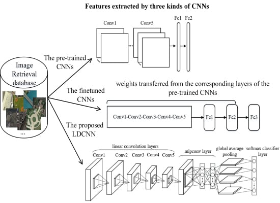
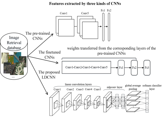
Learning powerful feature representations for image retrieval has always been a challenging task in the field of remote sensing. Traditional methods focus on extracting low-level hand-crafted features which are not only time-consuming but also tend to achieve unsatisfactory performance due to the complexity of remote sensing images. In this paper, we investigate how to extract deep feature representations based on convolutional neural networks (CNNs) for high-resolution remote sensing image retrieval (HRRSIR). To this end, several effective schemes are proposed to generate powerful feature representations for HRRSIR. In the first scheme, a CNN pre-trained on a different problem is treated as a feature extractor since there are no sufficiently-sized remote sensing datasets to train a CNN from scratch. In the second scheme, we investigate learning features that are specific to our problem by first fine-tuning the pre-trained CNN on a remote sensing dataset and then proposing a novel CNN architecture based on convolutional layers and a three-layer perceptron. The novel CNN has fewer parameters than the pre-trained and fine-tuned CNNs and can learn low dimensional features from limited labelled images. The schemes are evaluated on several challenging, publicly available datasets. The results indicate that the proposed schemes, particularly the novel CNN, achieve state-of-the-art performance.

1. Introduction

With the rapid development of remote sensing sensors over the past few decades, a considerable volume of high-resolution remote sensing images are now available. The high spatial resolution of the images makes detailed image interpretation possible, enabling a variety of remote sensing applications. However, efficiently organizing and managing the huge volume of remote sensing data remains a great challenge in the remote sensing community.

High-resolution remote sensing image retrieval (HRRSIR), which aims to retrieve and return images of interest from a large database, is an effective and indispensable method for the management of the large amount of remote sensing data. An integrated HRRSIR system roughly includes two components, feature extraction and similarity measure, and both play an important role in a successful system. Feature extraction focuses on the generation of powerful feature representations for the images, while similarity measure focuses on feature matching to determine the similarity between the query image and other images in the database.

We focus on feature extraction in this work since retrieval performance largely depends on whether the extracted features are representative. Traditional HRRSIR methods are mainly based on low-level feature representations, such as global features including spectral features [1], shape features [2], and especially texture features [3,4,5], which have been shown to be able to achieve satisfactory performance. In contrast to global features, local features are extracted from image patches centered at interesting or informative points and thus have desirable properties such as locality, invariance, and robustness. Remote sensing image analysis has benefited a lot from these desirable properties, and many methods have been developed for remote sensing registration and detection tasks [6,7,8]. In addition to these tasks, local features have also proven to be effective for HRRSIR. Yang et al. [9] investigated local invariant features for content-based geographic image retrieval for the first time. Extensive experiments on a publicly available dataset indicate the superiority of local features over global features such as simple statistics, color histogram, and homogeneous texture. However, both the global and local features mentioned above are low-level features. Moreover, they are hand-crafted, which likely limits how optimal they are as powerful feature representations.

Recently, deep learning methods have dramatically improved the state-of-the-art in speech recognition as well as object recognition and detection [10]. Content-based image retrieval has also benefited from the success of deep learning [11]. Researchers have explored the application of unsupervised deep learning methods for remote sensing recognition tasks such as scene classification [12] and image retrieval [13,14]. Unsupervised feature learning [13] has been used to learn sparse feature representations from remote sensing images directly for HRRSIR, but the performance is only slightly better than state-of-the-art. This is because the unsupervised learning framework is based on a shallow auto-encoder network with a single hidden layer making it incapable of generating sufficiently powerful feature representations. Deeper networks are necessary to generate powerful feature representations for HRRSIR.

Convolutional neural networks (CNNs), which consist of convolutional, pooling, and fully-connected layers, have already been regarded as the most effective deep learning approach to image analysis due to their remarkable performance on benchmark datasets such as ImageNet [15]. However, large numbers of labeled training samples as well as “tricks” to prevent overfitting are needed to train effective CNNs. In practice, a common strategy to address the training data issue is to transfer deep features from CNN models trained on problems for which there is enough labeled data, such as the ImageNet dataset for object recognition, and then apply them to the problem at hand such as scene classification [16,17,18] and image retrieval [19,20,21,22]. Alternately, in a recent work on transfer learning [23], instead of transferring the features from a pre-trained CNN, the authors use the scores obtained by the pre-trained deep neural networks to train a support vector machine (SVM) classifier. However, whether the deep feature representations extracted from such pre-trained CNN models can be used for HRRSIR remains an open question. The limited work on using pre-trained CNNs for remote sensing image retrieval [22] only considers features extracted from the last fully-connected layer. In contrast, we perform a thorough investigation on transfer learning for HRRSIR by considering features from both the fully-connected and convolutional layers, and from a wide range of CNN architectures. We further fine-tune the pre-trained CNNs to learn domain-specific features as well as propose a novel CNN architecture which has fewer parameters and learns low dimensional features from limited labelled images.

The main contributions of this paper are as follows:

• We propose two effective schemes to extract powerful deep features using CNNs for HRRSIR. In the first scheme, the pre-trained CNN is regarded as a feature extractor, and in the second scheme, a novel CNN architecture is proposed to learn low dimensional features.
• A thorough, comparative evaluation is conducted for a wide range of pre-trained CNNs using several remote sensing benchmark datasets. Three new challenging datasets are introduced to overcome the performance saturation of the existing benchmark dataset.
• The novel CNN is trained on a large remote sensing dataset and then applied to the other remote sensing datasets. The results show that replacing the fully-connected layers with a multi-layer perceptron not only decreases the number of parameters but also achieves remarkable performance with low dimensional features.
• The two schemes achieve state-of-the-art performance, establishing baseline results for future work on HRRSIR.

The remainder of the paper is organized as follows. An overview of CNNs, including the various pre-trained CNN models we consider, is presented in Section 2 and our specific HRRSIR methods are described in Section 3. Experimental results and analysis are presented in Section 4, and Section 5 includes a discussion. Section 6 concludes the findings of this study.

2. Convolutional Neural Networks (CNNs)

In this section, we first briefly introduce the typical architecture of CNNs and then review the pre-trained CNN models evaluated in our work.

2.1. The Architecture of CNNs

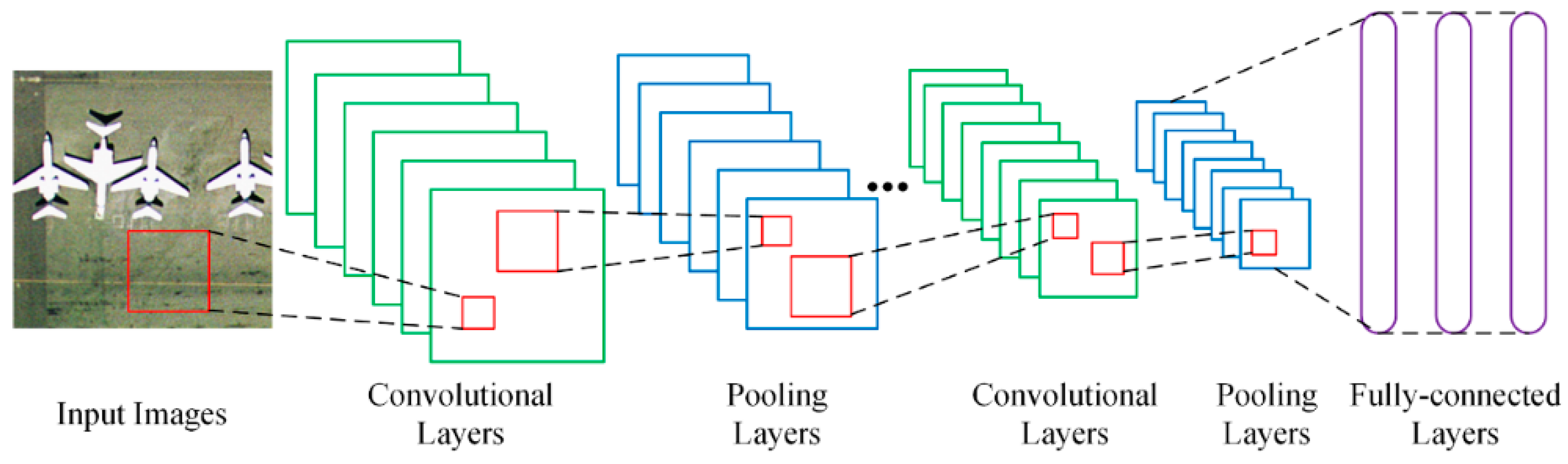
The main building blocks of a CNN architecture consist of different types of layers including convolutional layers, pooling layers, and fully-connected layers. There are generally a fixed number of filters (also called kernels, weights) in each convolutional layer which can output the same number of feature maps by sliding the filters through feature maps of the previous layer. The pooling layers perform subsampling along the spatial dimensions of the feature maps to reduce their size via max or average pooling. The fully-connected layers follow the convolutional and pooling layers. Figure 1 shows the typical architecture of a CNN model. Note that generally the element-wise rectified linear units (ReLU), i.e., $f(x)=\max (0,x)$, are applied to feature maps of both the convolutional and fully-connected layers to generate non-negative features. It is a commonly used activation function in CNN models due to its demonstrated improved performance over other activation functions [24,25].

2.2. The Pre-Trained CNN Models

Several successful CNN models pre-trained on ImageNet are evaluated in our work, namely the famous baseline model AlexNet [26], the Caffe reference model (CaffeRef) [27], the VGG network [28], and the VGG-VD network [29].

AlexNet is regarded as a baseline model, as it achieved the best performance in the ImageNet Large Scale Visual Recognition Challenge (ILSVRC-2012). The success of AlexNet is attributed to the large-scale labelled dataset, and techniques such as data augmentation, ReLU activation function, and dropout to reduce overfitting. Dropout is usually used in the first two fully-connected layers to reduce overfitting by randomly setting the output of each hidden neuron to zero with probability 0.5 [30]. AlexNet contains five convolutional layers followed by three fully-connected layers, providing guidance for the design and implementation of subsequent CNN models.

CaffeRef is a minor variation of AlexNet and is trained using the open-source deep learning framework Convolutional Architecture for Fast Feature Embedding (Caffe) [27]. The modifications of CaffeRef lie in the order of pooling and normalization layers as well as data augmentation strategy. It achieved similar performance on ILSVRC-2012 to AlexNet.

The VGG network includes three CNN models: VGGF, VGGM, and VGGS. These models explore different accuracy/speed trade-offs on benchmark datasets for image recognition and object detection. They have similar architectures with variations in the number and sizes of filters in the convolutional layers. The width of the final hidden layer determines the dimension of the feature representation when these models are used as feature extractors. This is equal to 4096 dimensions for the default model. Three variants models, VGGM128, VGGM1024, and VGGM2048, with narrower final hidden layers are used to investigate the effect of feature dimension. In order to speed up training, all the layers except for the second and third layer of VGGM are kept fixed during the training of these variants. These variants generate 128, 1024, and 2048 dimensional feature vectors, respectively.

Table 1. The architectures of the evaluated CNN Models. Conv1–5 are five convolutional layers and Fc1–3 are three fully-connected layers. For each of the convolutional layers, the first row specifies the number of filters and corresponding filter size as “size × size × number”; the second row indicates the convolution stride; and the last row indicates if Local Response Normalization (LRN) is used. For each of the fully-connected layers, its dimensionality is provided. In addition, dropout is applied to Fc1 and Fc2 to overcome overfitting.

Models	Conv1	Conv2	Conv3	Conv4	Conv5	Fc1	Fc2	Fc3
AlexNet	11 × 11 × 96	5 × 5 × 256	3 × 3 × 384	3 × 3 × 384	3 × 3 × 256	4096 dropout	4096 dropout	1000 softmax
	stride 4	stride 1	stride 1	stride 1	stride 1
	LRN	LRN	-	-	-
CaffeRef	11 × 11 × 96	5 × 5 × 256	3 × 3 × 384	3 × 3 × 384	3 × 3 × 256	4096 dropout	4096 dropout	1000 softmax
	stride 4	stride 1	stride 1	stride 1	stride 1
	LRN	LRN	-	-	-
VGGF	11 × 11 × 64	5 × 5 × 256	3 × 3 × 256	3 × 3 × 256	3 × 3 × 256	4096 dropout	4096 dropout	1000 softmax
	stride 4	stride 1	stride 1	stride 1	stride 1
	LRN	LRN	-	-	-
VGGM	7 × 7 × 96	5 × 5 × 256	3 × 3 × 512	3 × 3 × 512	3 × 3 × 512	4096 dropout	4096 dropout	1000 softmax
	stride 2	stride 2	stride 1	stride 1	stride 1
	LRN	LRN	-	-	-
VGGM-128	7 × 7 × 96	5 × 5 × 256	3 × 3 × 512	3 × 3 × 512	3 × 3 × 512	4096 dropout	128 dropout	1000 softmax
	stride 2	stride 2	stride 1	stride 1	stride 1
	LRN	LRN	-	-	-
VGGM-1024	7 × 7 × 96	5 × 5 × 256	3 × 3 × 512	3 × 3 × 512	3 × 3 × 512	4096 dropout	1024 dropout	1000 softmax
	stride 2	stride 2	stride 1	stride 1	stride 1
	LRN	LRN	-	-	-
VGGM-2048	7 × 7 × 96	5 × 5 × 256	3 × 3 × 512	3 × 3 × 512	3 × 3 × 512	4096 dropout	2048 dropout	1000 softmax
	stride 2	stride 2	stride 1	stride 1	stride 1
	LRN	LRN	-	-	-
VGGS	7 × 7 × 96	5 × 5 × 256	3 × 3 × 512	3 × 3 × 512	3 × 3 × 512	4096 dropout	4096 dropout	1000 softmax
	stride 2	stride 1	stride 1	stride 1	stride 1
	LRN	-	-	-	-

summarizes the different architectures of these CNN models. We refer the reader to the relevant papers for more details.

VGG-VD is a very deep CNN network including VD16 (16 weight layers including 13 convolutional layers and 3 fully-connected layers) and VD19 (19 weight layers including 16 convolutional layers and 3 fully-connected layers). These two models were developed to investigate the effect of network depth on large-scale image recognition task. It has been demonstrated that the representations extracted by VD16 and VD19 generalize well to datasets other than those on which they were trained.

3. Deep Feature Representations for HRRSIR

In this section, we present the two proposed schemes for HRRSIR in detail. The package MatConvNet (http://www.vlfeat.org/matconvnet/) is used for the proposed schemes [31]. The pre-trained CNN models we use are available at (http://www.vlfeat.org/matconvnet/pretrained/).

3.1. First Scheme: Features Extracted by the Pre-Trained CNN without Labelled Images

It is not possible to train an effective CNN without a sufficient, usually large number of labelled images. However, many works have shown that the features extracted by a pre-trained CNN generalize well to datasets from different domains. Therefore, in the first scheme, we regard pre-trained CNNs as feature extractors. This does not require any labelled remote sensed images for training.

The deep features are extracted directly from specific layers of the pre-trained CNN models. In order to improve performance, preprocessing steps such as data augmentation and mean subtraction are widely used. Data augmentation is a commonly used technique to augment the training samples through image cropping, flipping, and rotating, etc. Mean subtraction subtracts the average image computed over all the training samples. This speeds up the convergence of the network during training. In our work, we just conduct mean subtraction with the mean value provided by corresponding pre-trained CNN.

3.1.1. Features Extracted from Fully-Connected Layers

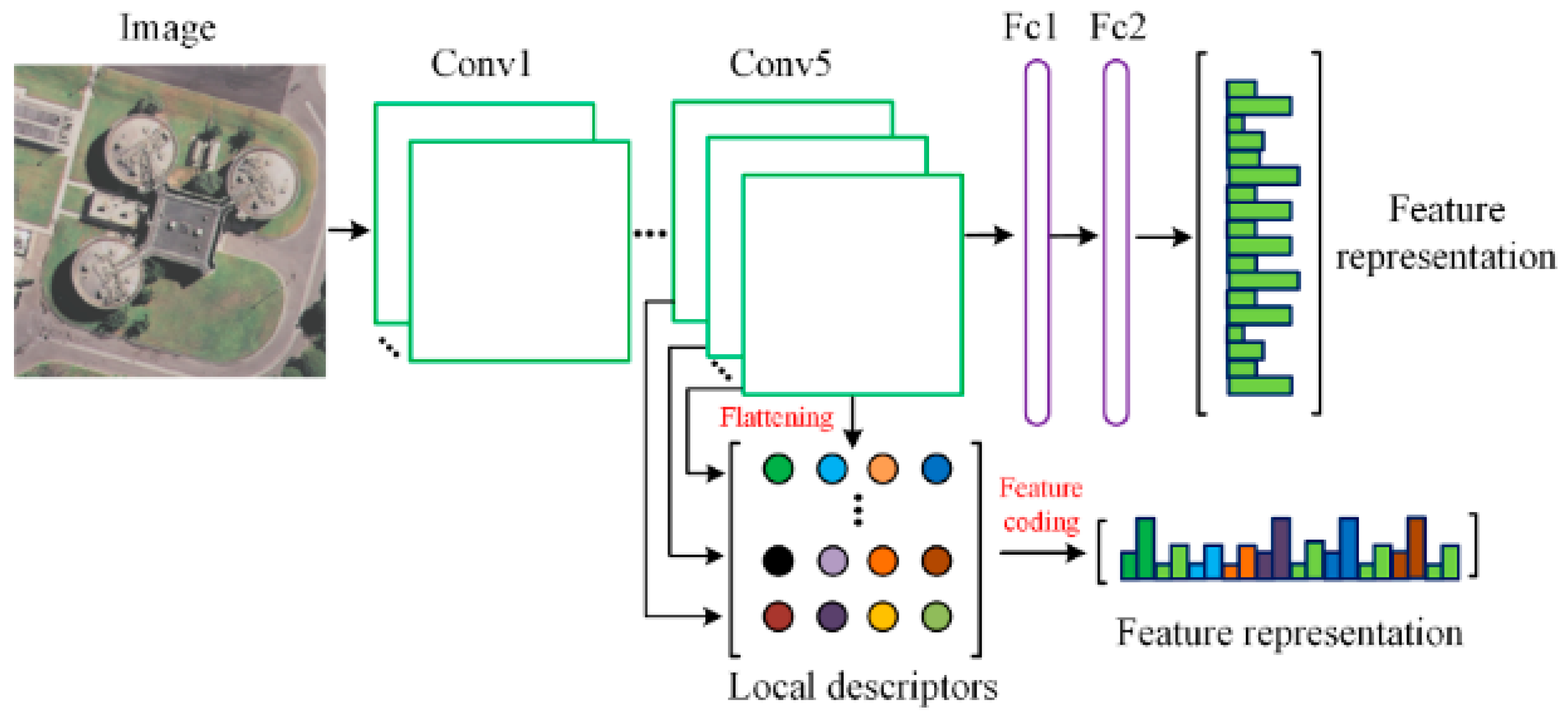
Though there are three fully-connected layers in a pre-trained CNN model, the last layer (Fc3) is usually fed into a softmax (normalized exponential) activation function for classification. Therefore, the first two layers (Fc1 and Fc2) are used to extract features in this work, as shown in Figure 2. Fc1 and Fc2 each generate a 4096-D dimensional feature representation for all the evaluated models except for the three variants of VGGM. These 4096-D feature vectors can be directly used for computing the similarity between images for image retrieval.

3.1.2. Features Extracted from Convolutional Layers

Fc features can be considered as global features to some extent, while previous works have demonstrated that local features have better performance than global features when used for HRRSIR [9,32]. Therefore, it is important to investigate whether CNNs can generate local features and how to aggregate these local descriptors into a compact feature vector. There has been some work that investigates how to generate compact features from the activations of the fully-connected layers [33] and the convolutional layers [34].

Feature maps of the current convolutional layer are computed by sliding the filters over the output feature maps of the previous layer with a fixed stride, and thus each unit of a feature map corresponds to a local region of the image. To compute the feature representation of this local region, the units of these feature maps need to be recombined. Figure 2 illustrates the process of extracting features from the last convolutional layer (e.g., Conv5 layer in this case). The feature maps are firstly flattened to obtain a set of feature vectors. Each column then represents a local descriptor which can be regarded as the feature representation of the corresponding image region. Let $n$ and $m$ be the number and the size of feature maps, respectively. The local descriptors can be defined by:

$$F=[x_1,x_2,...,x_m]$$

(1)

where $x_i(i=1,2,...,m)$ is an n-dimensional feature vector representing a local descriptor.

The local descriptor set $F$ is of high dimension, thereby using it directly for similarity measure is not possible. We therefore utilize bag of visual words (BOVW) [35], vector of locally aggregated descriptors (VLAD) [36], and improved fisher kernel (IFK) [37] to aggregate these local descriptors into a compact feature vector. BOVW is extracted by quantizing local descriptors into visual words in a dictionary which is generally formed using clustering algorithms (e.g., K-means). IFK uses Gaussian mixture models to encode local feature descriptors, which are formed by concatenating the partial derivatives of the mean and variance of the Gaussian functions. VLAD is a simplification of IFK which uses the non-probabilistic K-means clustering to generate the dictionary. The differences between each local descriptor and its nearest neighbor in the dictionary are accumulated to obtain the feature vector.

3.2. Second Scheme: Learning Domain-Specific Features with Limited Labelled Images

Though pre-trained CNNs have been shown to generalize well to datasets from domains different than on which they were trained, we here ask the question: can we improve the performance of the pre-trained CNN if we have limited labelled images? In the second scheme, we propose two approaches to solve this problem.

3.2.1. Features Extracted by Fine-Tuned CNNs

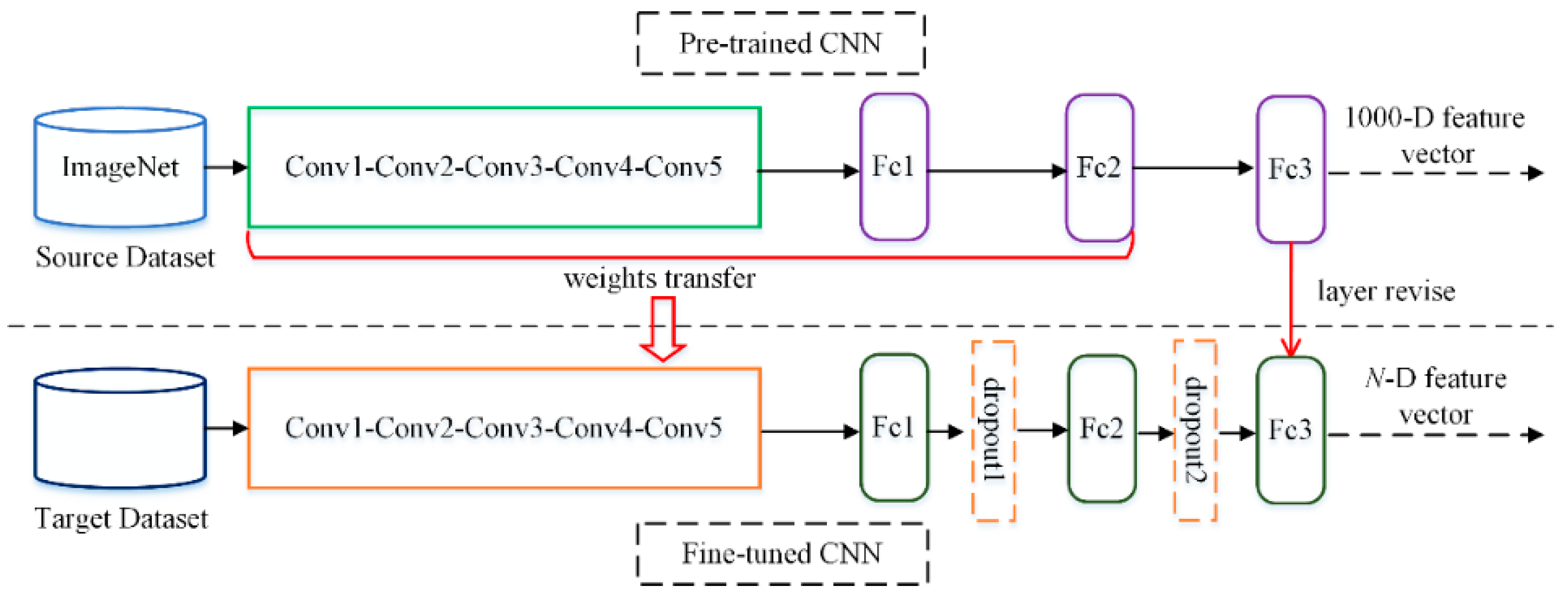
The first approach is to fine-tune the CNNs pre-trained on ImageNet using the target remote sensing dataset. This will adjust the trained parameters to better suit the target dataset. Figure 3 shows the flowchart of fine-tuning the pre-trained CNN on the target dataset. The weights of the pre-trained CNN can be directly transferred to the fine-tuned CNN as initialization for training.

The pre-trained and fine-tuned CNN models have the same number of convolutional and fully-connected layers but differ greatly in the number of outputs in the Fc3 layer. The last fully-connected layer (Fc3) of a CNN model is used for classification, thus the number of units in this layer is equal to the number of image classes in the dataset.

3.2.2. Features Extracted by the Novel Low Dimensional CNN (LDCNN)

In the first scheme, pre-trained CNNs are used as feature extractors to extract Fc and Conv features for HRRSIR, but these models are trained on ImageNet, which is very different from remote sensing images. In practice, a common strategy for this problem is to fine-tune the pre-trained CNNs on the target remote sensing dataset to learn domain-specific features. However, the deep features extracted from the fine-tuned Fc layers are usually 4096-D feature vectors, which are not compact enough for large-scale image retrieval. Further, the Fc layers are prone to overfitting because most of the parameters lie in Fc layers. In addition, the convolutional filters in CNN are generalized linear models (GLMs) based on the assumption that the features are linearly separable, while features that achieve good abstraction are generally highly nonlinear functions of the input.

Network in Network (NIN) [38], which is a stack of several mlpconv layers, has therefore been proposed to overcome these limitations. In NIN, the GLM is replaced with an mlpconv layer to enhance model discriminability and the conventional fully-connected layers are replaced with global average pooling to directly output the spatial averages of the feature maps from the last mlpconv layer which are then fed into the softmax layer for classification. We refer the reader to [38] for more details.

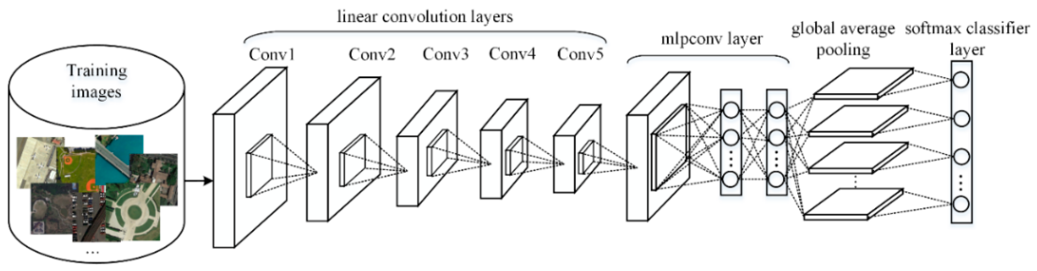
Inspired by NIN, we propose a novel CNN that has high model discriminability but generates low dimensional features. Figure 4 shows the overall structure of the low dimensional CNN (LDCNN) which consists of five conventional convolution layers, an mlpconv layer, a global average pooling layer, and a softmax classifier layer. LDCNN is essentially the combination of a conventional CNN (linear convolution layer) and an NIN (mlpconv layer). The structure design is based on the assumption that in conventional CNNs the earlier layers are trained to learn low-level features such as edges and corners that are linearly separable while the later layers are trained to learn more abstract high-level features that are nonlinearly separable. The mlpconv layer we use in this paper is a three-layer perceptron trainable by back-propagation and is able to generate one feature map for each corresponding class. The global average pooling layer computes the average of each feature map and leads to an n-dimensional feature vector (n is the number of image classes) which will be used for HRRSIR in this paper.

4. Experiments and Analysis

In this section, we evaluate the performance of the proposed schemes for HRRSIR on several publicly available remote sensing image datasets. We first introduce the datasets and experimental setup and then present the experimental results in detail.

4.1. Datasets

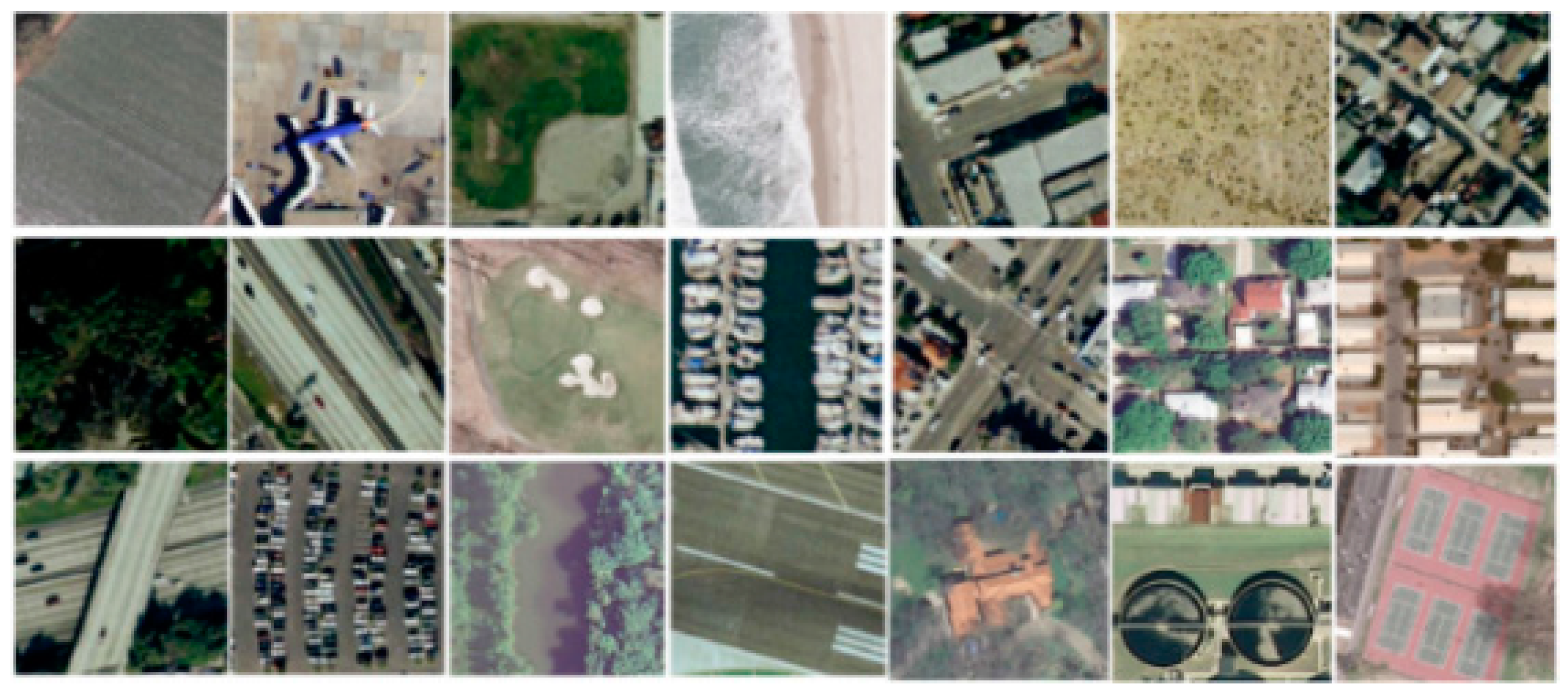
The University of California, Merced dataset (UCMD) (http://vision.ucmerced.edu/datasets/landuse.html) is a challenging dataset containing 21 image classes: agricultural, airplane, baseball diamond, beach, buildings, chaparral, dense residential, forest, freeway, golf course, harbor, intersection, medium density residential, mobile home park, overpass, parking lot, river, runway, sparse residential, storage tanks, and tennis courts [9]. Each class has 100 images with the size of 256 × 256 pixels and about one foot spatial resolution. This dataset is cropped from large aerial images downloaded from the United States Geological Survey (USGS). Figure 5 shows some sample images from this dataset.

The WHU-RS19 remote sensing dataset (RSD) (http://dsp.whu.edu.cn/cn/staff/yw/HRSscene.html) is collected from Google Earth imagery and consists of 19 classes: airport, beach, bridge, commercial area, desert, farmland, football field, forest, industrial area, meadow, mountain, park, parking, pond, port, railway station, residential area, river, and viaduct [39]. The dataset contains a total of 1005 images and each image has a fixed size of 600 × 600 pixels. The spatial resolution is up to half a meter. Figure 6 shows some sample images from this dataset.

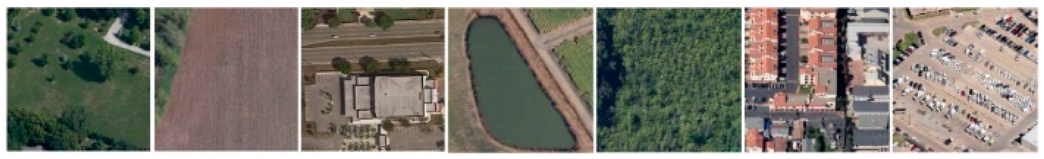
The RSSCN7 dataset (https://www.dropbox.com/s/j80iv1a0mvhonsa/RSSCN7.zip?dl=0) consists of seven land-use classes: grassland, forest, farmland, parking lot, residential region, industrial region, river, and lake [40]. For each class, there are 400 images with the size of 400 × 400 pixels sampled on four different scale levels from Google Earth. Figure 7 shows some sample images from this dataset.

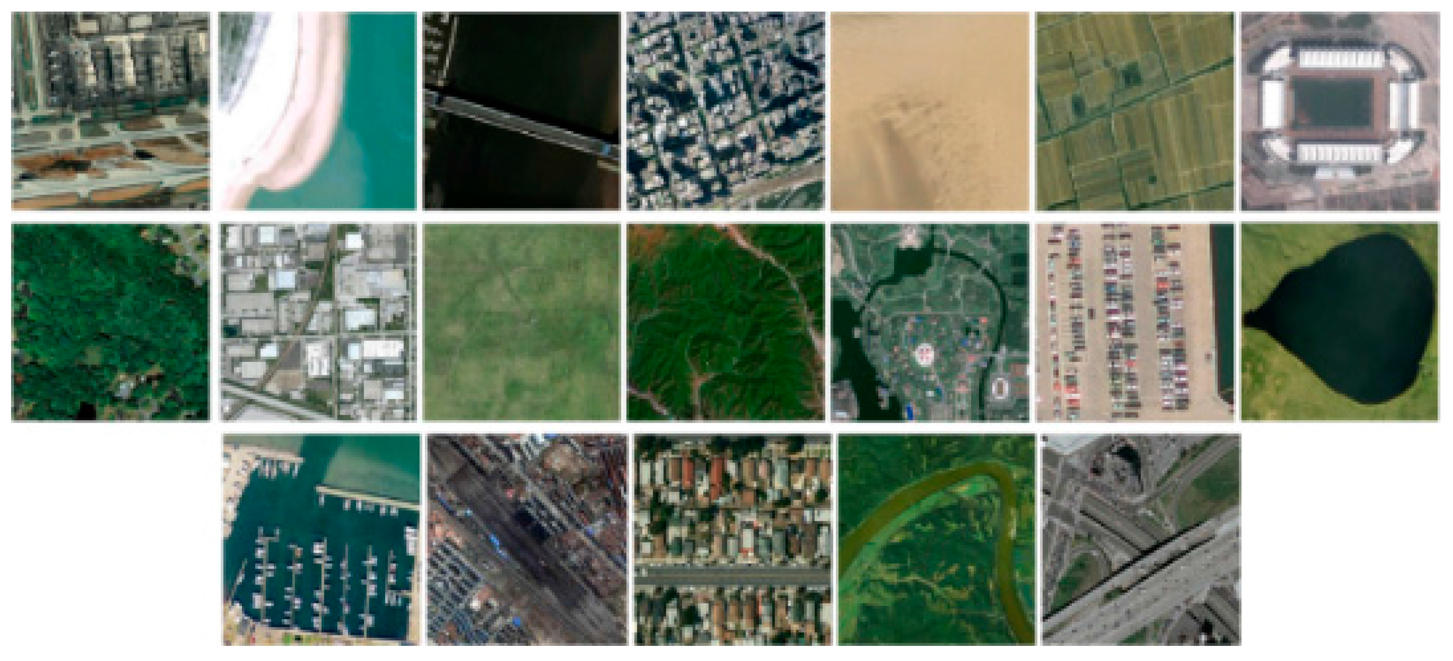
The aerial image dataset (AID) (http://www.lmars.whu.edu.cn/xia/AID-project.html) is a large-scale publicly available dataset [41]. It is notably larger than the three datasets mentioned above. It is collected with the goal of advancing the state-of-the-art in scene classification of remote sensing images. The dataset consists of 30 scene types: airport, bare land, baseball field, beach, bridge, center, church, commercial, dense residential, desert, farmland, forest, industrial, meadow, medium residential, mountain, park, parking, playground, pond, port, railway station, resort, river, school, sparse residential, square, stadium, storage tanks, and viaduct. The dataset contains a total of 10,000 images. Each class has 220 to 420 images of size 600 × 600 pixels. This dataset is very challenging since its spatial resolution varies greatly between around 0.5 to 8 m. Figure 8 shows some samples images from AID.

UCMD has been widely used for image retrieval performance evaluation. However, it is relatively small and so the performance on this dataset has saturated. In contrast to UCMD, the other three datasets are more challenging due to the image scale, image size, and spatial resolution.

4.2. Experimental Setup

4.2.1. Implementation Details

The images are resized to 227 × 227 pixels for AlexNet and CaffeRef and to 224 × 224 pixels for the other networks, as these are the required input dimensions of CNNs. K-means clustering is used to construct the dictionaries for aggregating the Conv features. The dictionary sizes of BOVW, VLAD, and IFK are empirically set to 1000, 100, and 100, respectively.

Regarding the fine-tuning process, the weights of the convolutional layers and the first two fully-connected layers are transferred from the pre-trained CNN model, while the weights of the last fully-connected layer are initialized from a Gaussian distribution (with a mean of 0 and a standard deviation of 0.01).

In the case of LDCNN, the weights of the five convolutional layers are transferred from VGGM. We also tried using AlexNet, CaffeRef, VGGF, and VGGS but achieved comparable or slightly worse performance. The weights of convolutional layers are kept fixed during training in order to speed up training with the limited number of labelled remote sensing images. More specially, the layers after the last pooling layer of VGGM are removed and the remaining layers are preserved for LDCNN. The weights of the mlpconv layer are initialized from a Gaussian distribution (with a mean of 0 and a standard deviation is 0.01). The initial learning rate is set to 0.001 and is lowered by a factor of 10 when the accuracy on the validation set stops improving. Dropout is applied to the mlpconv layer.

The AID dataset is used to fine-tune the pre-trained CNNs and to train the LDCNN because it is the largest of the remote sensed datasets, having 10,000 images in total. The training data consists of 80% of the images per class selected at random. The remaining images constitute the validation data used to indicate when to stop training.

In the following experiments, we perform 2100 queries for the UCMD dataset, 1005 queries for the RSD dataset, 2800 queries for the RSSCN7 dataset, and 10,000 queries for the AID dataset. Euclidean distance is used as the similarity measure, and all the feature vectors are L2 normalized before similarity measure.

4.2.2. Performance Measures

The average normalized modified retrieval rank (ANMRR) and mean average precision (mAP) are used to evaluate the retrieval performance.

Let $q$ be a query image with the ground truth size of $NG(q)$, $R(k)$ be the retrieved rank of the k-th image, which is defined as

$$R(k)=\{\begin{array}{l}R(k),R(k)\le K(q)\\ 1.25K(q),R(k)>K(q)\end{array}$$

(2)

where $K(q)=2NG(q)$ is used to impose a penalty on the retrieved images with a higher rank. The normalized modified retrieval rank (NMRR) is defined as

$$NMRR(q)=\frac{AR(q)-0.5[1+NG(q)]}{1.25K(q)-0.5[1+NG(q)]}$$

(3)

where $AR(q)=\frac{1}{NG(q)}{\displaystyle \sum _{k=1}^{NG(q)}R(k)}$ is the average rank. Then the final ANMRR can be defined as

$$ANMRR=\frac{1}{NQ}{\displaystyle \sum _{q=1}^{NQ}NMRR(q)}$$

(4)

where $NQ$ is the number of queries. ANMRR ranges from zero to one, and a lower value means better retrieval performance.

Given a set of $Q$ queries, mAP is defined as

$$mAP=\frac{{\displaystyle {\sum }_{q=1}^{Q}AveP(q)}}{Q}$$

(5)

where AveP is the average precision defined as

$$AveP=\frac{{\displaystyle {\sum }_{k=1}^n(P(k)\times rel(k))}}{numberofrelevantimages}$$

(6)

where $P(k)$ is the precision at cutoff $k$, $rel(k)$ is an indicator function equaling 1 if the image at rank is a relevant image and zero if otherwise. $k$ and $n$ are the rank and number of the retrieved images, respectively. Note that the average is over all relevant images.

We also use precision at k (P@k) as an auxiliary performance measure in the case that ANMRR and mAP achieve opposite results. Precision is defined as the fraction of retrieved images that are relevant to the query image.

4.3. Results of the First Scheme

4.3.1. Results of Fc Features

The results of using Fc features on the four datasets are shown in

Table 2. The performances of Fc features (ReLU is used) extracted by different CNN models on the four datasets. For average normalized modified retrieval rank (ANMRR), lower values indicate better performance, while for mean average precision (mAP), larger is better. The best result for each dataset is reported in bold.

Features	UCMD		RSD		RSSCN7		AID
	ANMRR	mAP	ANMRR	mAP	ANMRR	mAP	ANMRR	mAP
AlexNet_Fc1	0.447	0.4783	0.332	0.5960	0.474	0.4120	0.548	0.3532
AlexNet_Fc2	0.410	0.5113	0.304	0.6206	0.446	0.4329	0.534	0.3614
CaffeRef_Fc1	0.429	0.4982	0.305	0.6273	0.446	0.4381	0.532	0.3692
CaffeRef_Fc2	0.402	0.5200	0.283	0.6460	0.433	0.4474	0.526	0.3694
VGGF_Fc1	0.417	0.5116	0.302	0.6283	0.450	0.4346	0.534	0.3674
VGGF_Fc2	0.386	0.5355	0.288	0.6399	0.440	0.4400	0.527	0.3694
VGGM_Fc1	0.404	0.5235	0.305	0.6241	0.442	0.4479	0.526	0.3760
VGGM_Fc2	0.378	0.5444	0.300	0.6255	0.440	0.4412	0.533	0.3632
VGGM128_Fc1	0.435	0.4863	0.356	0.5599	0.465	0.4176	0.582	0.3145
VGGM128_Fc2	0.498	0.4093	0.463	0.4393	0.513	0.3606	0.676	0.2183
VGGM1024_Fc1	0.413	0.5138	0.321	0.6052	0.454	0.4380	0.542	0.3590
VGGM1024_Fc2	0.400	0.5165	0.330	0.5891	0.447	0.4337	0.568	0.3249
VGGM2048_Fc1	0.414	0.5130	0.317	0.6110	0.455	0.4365	0.536	0.3662
VGGM2048_Fc2	0.388	0.5315	0.316	0.6053	0.446	0.4357	0.552	0.3426
VGGS_Fc1	0.410	0.5173	0.307	0.6224	0.449	0.4406	0.526	0.3761
VGGS_Fc2	0.381	0.5417	0.296	0.6288	0.441	0.4412	0.523	0.3725
VD16_Fc1	0.399	0.5252	0.316	0.6102	0.444	0.4354	0.548	0.3516
VD16_Fc2	0.394	0.5247	0.324	0.5974	0.452	0.4241	0.568	0.3272
VD19_Fc1	0.408	0.5144	0.336	0.5843	0.454	0.4243	0.554	0.3457
VD19_Fc2	0.398	0.5195	0.342	0.5736	0.457	0.4173	0.570	0.3255

. For the UCMD dataset, the best result is obtained by using the Fc2 features of VGGM, which achieves an ANMRR value that is about 12% lower and a mAP value that is about 14% higher than that of the worst result which is achieved by VGGM128_Fc2. For the RSD dataset, the best result is obtained by using the Fc2 features of CaffeRef, which achieves an ANMRR value that is about 18% lower and a mAP value that is about 21% higher than that of the worst result, which is achieved by VGGM128_Fc2.

Note that sometimes the two performance measures ANMRR and mAP indicate “opposite” results. For example, VGGF_Fc2 and VGGM_Fc2 achieve better results on the RSSCN7 dataset than the other features in terms of ANMRR value, while VGGM_Fc1 performs the best on the RSSCN7 dataset in terms of mAP value. Such “opposite” results can also be found on the AID dataset in terms of VGGS_Fc1 and VGGS_Fc2 features. Here P@k is used to further investigate the performance of the features, as shown in

Table 3. The precision at k (P@k) values of Fc features that achieve inconsistent results on the RSSCN7 and AID datasets for the ANMRR and mAP measures.

Measures	RSSCN7			AID
	VGGF_Fc2	VGGM_Fc1	VGGM_Fc2	VGGS_Fc1	VGGS_Fc2
P@5	0.7974	0.8098	0.8007	0.7754	0.7685
P@10	0.7645	0.7787	0.7687	0.7415	0.7346
P@50	0.6618	0.6723	0.6626	0.6265	0.6214
P@100	0.5940	0.6040	0.5943	0.5550	0.5521
P@1000	0.2960	0.2915	0.2962	0.2069	0.2097

. When the number of retrieved images k is 100 or smaller, we see that the Fc features of VGGM and in particular VGGM_Fc1 perform slightly better than VGGF_Fc2 in the case of the RSSCN7 dataset, and in the case of the AID dataset, VGGS_Fc1 performs slightly better than VGGS_Fc2.

It is interesting that VGGM performs better than its three variants on the four datasets, indicating the lower dimension of the Fc2 features does not improve the performance. However, in contrast to VGGM, these three variants have reduced storage and time cost due to the lower feature dimension. It can be also observed that Fc2 features perform better than the Fc1 features for most of the evaluated CNN models on the four datasets.

4.3.2. Results of Conv Features

Table 4. The performance of the Conv features (ReLU is used) aggregated using bag of visual words (BOVW), vector of locally aggregated descriptors (VLAD), and improved fisher kernel (IFK) on the four datasets. For ANMRR, lower values indicate better performance, while for mAP, larger is better. The best result for each dataset is reported in bold.

Features	UCMD		RSD		RSSCN7		AID
	ANMRR	mAP	ANMRR	mAP	ANMRR	mAP	ANMRR	mAP
AlexNet_BOVW	0.594	0.3240	0.539	0.3715	0.552	0.3403	0.699	0.2058
AlexNet_VLAD	0.551	0.3538	0.419	0.4921	0.465	0.4144	0.616	0.2793
AlexNet_IFK	0.500	0. 4217	0.417	0.4958	0.486	0.4007	0.642	0.2592
CaffeRef_BOVW	0.571	0.3416	0.493	0.4128	0.493	0.3858	0.675	0.2265
CaffeRef_VLAD	0.563	0.3396	0.364	0.5552	0.428	0.4543	0.591	0.3047
CaffeRef_IFK	0.461	0.4595	0.364	0.5562	0.428	0.4628	0.601	0.2998
VGGF_BOVW	0.554	0.3578	0.479	0.4217	0.486	0.3926	0.682	0.2181
VGGF_VLAD	0.553	0.3483	0.374	0.5408	0.444	0.4352	0.604	0.2895
VGGF_IFK	0.475	0.4464	0.397	0.5141	0.454	0.4327	0.620	0.2769
VGGM_BOVW	0.590	0.3237	0.531	0.3790	0.549	0.3469	0.699	0.2054
VGGM_VLAD	0.531	0.3701	0.352	0.5640	0.420	0.4621	0.572	0.3200
VGGM_IFK	0.458	0.4620	0.382	0.5336	0.431	0.4516	0.605	0.2955
VGGM128_BOVW	0.656	0.2717	0.606	0.3120	0.596	0.3152	0.743	0.1728
VGGM128_VLAD	0.536	0.3683	0.373	0.5377	0.436	0.4411	0.602	0.2891
VGGM128_IFK	0.471	0.4437	0.424	0.4834	0.442	0.4388	0.649	0.2514
VGGM1024_BOVW	0.622	0.2987	0.558	0.3565	0.564	0.3393	0.714	0.1941
VGGM1024_VLAD	0.535	0.3691	0.358	0.5560	0.425	0.4568	0.577	0.3160
VGGM1024_IFK	0.454	0.4637	0.399	0.5149	0.436	0.4490	0.619	0.2809
VGGM2048_BOVW	0.609	0.3116	0.548	0.3713	0.566	0.3378	0.715	0.1939
VGGM2048_VLAD	0.531	0.3728	0.354	0.5591	0.423	0.4594	0.576	0.3150
VGGM2048_IFK	0.456	0.4643	0.376	0.5387	0.430	0.4535	0.610	0.2907
VGGS_BOVW	0.615	0.3021	0.521	0.3843	0.522	0.3711	0.670	0.2347
VGGS_VLAD	0.526	0.3763	0.355	0.5563	0.428	0.4541	0.555	0.3396
VGGS_IFK	0.453	0.4666	0.368	0.5497	0.428	0.4574	0.596	0.3054
VD16_BOVW	0.518	0.3909	0.500	0.3990	0.478	0.3930	0.677	0.2236
VD16_VLAD	0.533	0.3666	0.342	0.5724	0.426	0.4436	0.554	0.3365
VD16_IFK	0.407	0.5102	0.368	0.5478	0.436	0.4405	0.594	0.3060
VD19_BOVW	0.530	0.3768	0.509	0.3896	0.498	0.3762	0.673	0.2253
VD19_VLAD	0.514	0.3837	0.358	0.5533	0.439	0.4310	0.562	0.3305
VD19_IFK	0.423	0.4908	0.375	0.5411	0.440	0.4375	0.604	0.2965

shows the results of the Conv features aggregated using BOVW, VLAD, and IFK on the four datasets. For the UCMD dataset, IFK performs better than BOVW and VLAD for all the evaluated CNN models and the best result is achieved by VD16 (ANMRR 0.407). It can also be observed that BOVW performs the worst except for VD16. This makes sense because BOVW ignores spatial information which is very important for remote sensing images when encoding local descriptors into a compact feature vector. For the other three datasets, VLAD has better performance than BOVW and IFK for most of the evaluated CNN models and the best results on the RSD, RSSCN7, and AID datasets are achieved by VD16 (ANMRR 0.342), VGGM (ANMRR 0.420) and VD16 (ANMRR 0.554), respectively. Moreover, we can see BOVW still has the worst performance among these three feature aggregation methods.

Similar to the Fc features, the Conv features also achieve some “opposite” results on the RSSCN7 and AID datasets. For example, VGGM_VLAD performs the best on the RSSCN7 dataset in terms of ANMRR value, while CaffeRef_IFK outperforms the other features in terms of mAP value. The “opposite” results can also be found on the AID dataset with respect to the VD16_VLAD and VGGS_VLAD features. Here P@k is also used to further investigate the performances of these features, as shown in

Table 5. The P@k values of Conv features that achieve inconsistent results on the RSSCN7 and AID datasets for the ANMRR and mAP measures.

Measures	RSSCN7		AID
	CaffeRef_IFK	VGGM_VLAD	VGGS_VLAD	VD16_VLAD
P@5	0.7741	0.7997	0.7013	0.6870
P@10	0.7477	0.7713	0.6662	0.6577
P@50	0.6606	0.6886	0.5649	0.5654
P@100	0.6024	0.6294	0.5049	0.5081
P@1000	0.2977	0.2957	0.2004	0.1997

. It is clear that VGGM_VLAD achieves better performance than CaffeRef_IFK when the number of retrieved images is 100 or smaller. In the case of the AID dataset, VGGS_VLAD has better performance when the number of retrieved images is 10 or smaller or is 1000.

4.3.3. Effect of ReLU on Fc and Conv Features

The Fc and Conv features can be extracted either with or without the use of the ReLU transformation. Deep features with ReLU means ReLU is applied to generate non-negative features which can improve the nonlinearity of the features, while deep features without ReLU mean the opposite. To give an extensive evaluation of deep features, the effect of ReLU on the Fc and Conv features is investigated.

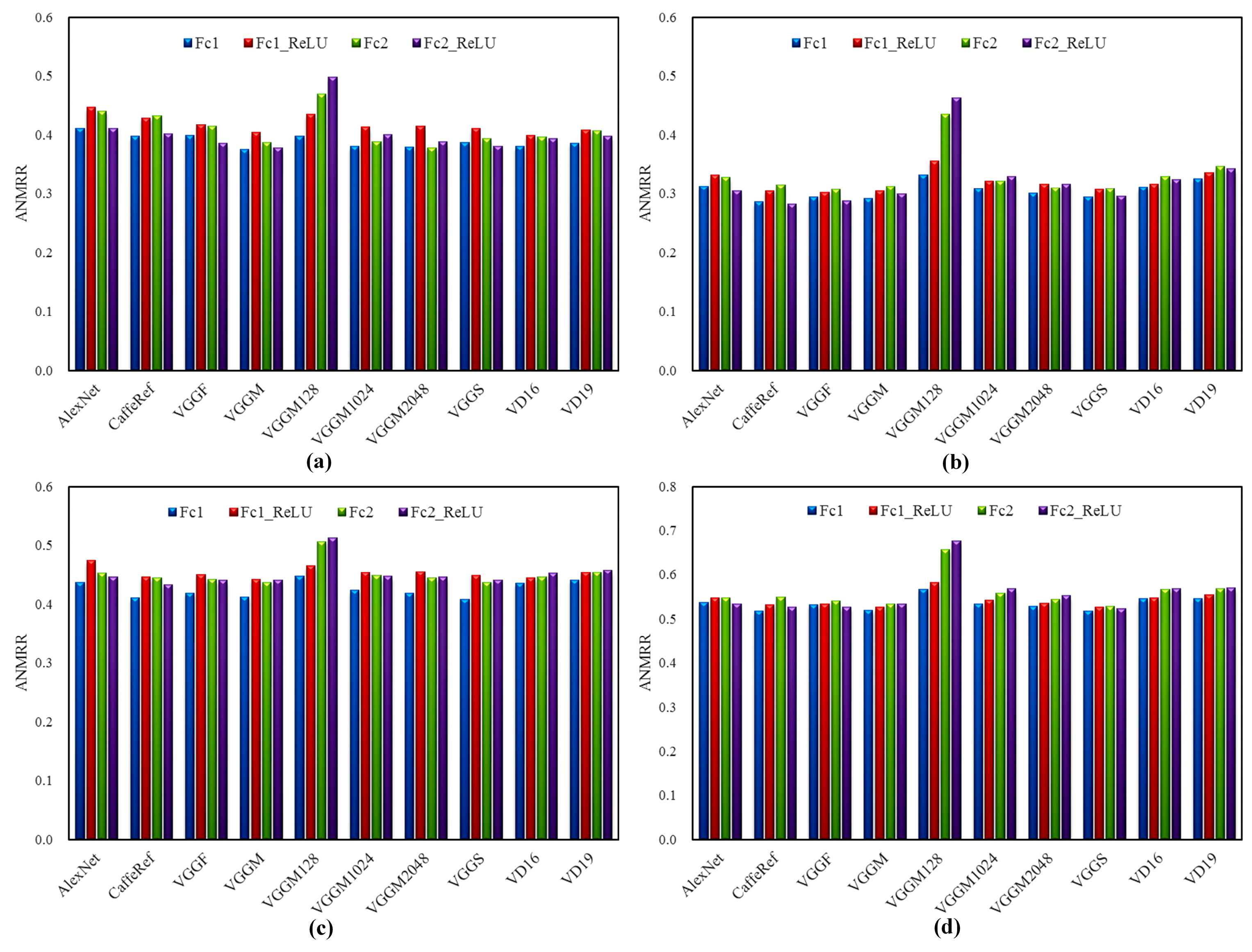
Figure 9 shows the results of Fc features extracted by different CNN models with and without ReLU on the four datasets. We can see that Fc1 features (without ReLU) perform better than Fc1_ReLU features, indicating the nonlinearity does not contribute to the performance improvement as expected. However, we tend to achieve opposite results (Fc2_ReLU achieves better or similar performance compared with Fc2) in terms of Fc2 and Fc2_ReLU features except for VGGM128, VGGM1024, and VGGM2048. A possible explanation is that the Fc2 layer can generate higher-level features which are then used as input of the classification layer (Fc3 layer) and thus improving nonlinearity will benefit the final results.

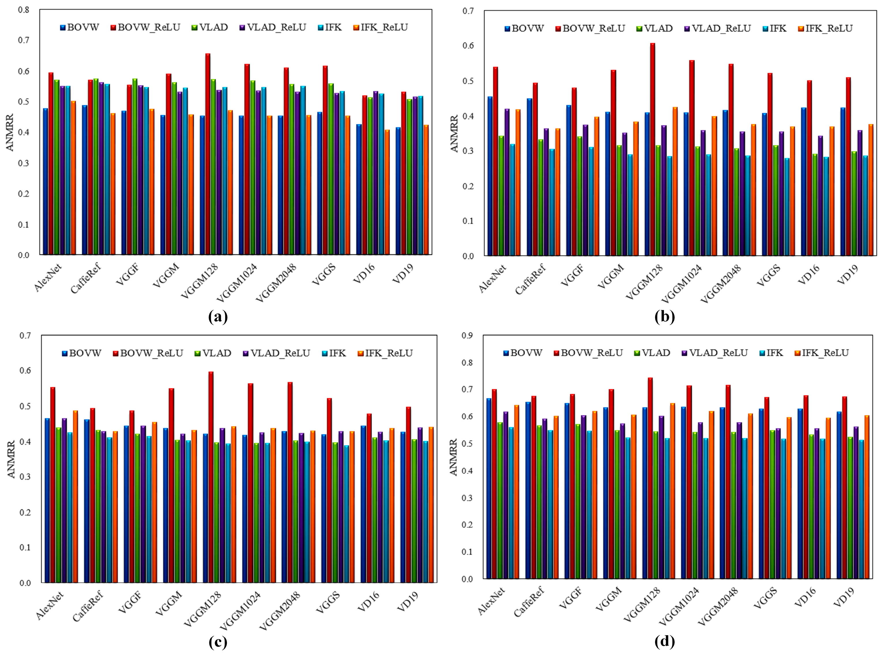
Figure 10 shows the results of Conv features aggregated by BOVW, VLAD, and IFK on the four datasets. It can be observed that the use of ReLU (BOVW_ReLU, VLAD_ReLU, and IFK_ReLU) decreases the performance of the evaluated CNN models on the four datasets except for the UCMD dataset. Regarding the UCMD dataset, the use of ReLU decreases the performance in the case of BOVW but improves the performance in the case of VLAD (except for VD16 and VD19) and IFK. In addition, it is interesting to find that BOVW achieves better performance than VLAD and IFK on the UCMD dataset and IFK performs better than BOVW and VLAD on the other three datasets in terms of Conv features without the use of ReLU.

Table 6. The models that achieve the best results in terms of Fc and Conv features on each dataset. The numbers are ANMRR values.

Features	UCMD		RSD		RSSCN7		AID
Fc1	VGGM	0.375	Caffe_Ref	0.286	VGGS	0.408	VGGS	0.518
Fc1_ReLU	VD16	0.399	VGGF	0.302	VGGM	0.442	VGGS	0.526
Fc2	VGGM2048	0.378	VGGF	0.307	VGGS	0.437	VGGS	0.528
Fc2_ReLU	VGGM	0.378	Caffe_Ref	0.283	Caffe_Ref	0.433	VGGS	0.523
Conv	VD19	0.415	VGGS	0.279	VGGS	0.388	VD19	0.512
Conv_ReLU	VD16	0.407	VD16	0.342	VGGM	0.420	VD16	0.554

shows the best results of Fc and Conv features on the four benchmark datasets. The models that achieve these results are also shown in the table. It is interesting to find that the very deep models (VD16 and VD19) perform worse than the relatively shallow models in terms of Fc features but perform better in terms of Conv features. These results indicate that network depth has an effect on the retrieval performance. Specially, increasing the convolutional layer depth will improve the performance of Conv features but will decrease the performance of Fc features. For example, VD16 has 13 convolutional layers and 3 fully-connected layers while VGGS has 5 convolutional layers and 3 fully-connected layers. However, VD16 achieves better performance on the AID dataset in terms of Conv features but achieves worse performance in terms of Fc features. This makes sense because the Fc layers can generate high-level domain-specific features while the Conv layers can generate more generic features. In addition, more data and techniques are needed in order to train a successful very deep model such as VD16 and VD19 than the relatively shallow models. Moreover, very deep models will also have higher time costs than relatively shallow models. Therefore, it is wise to balance the tradeoff between the performance and efficiency in practice, especially for large-scale tasks such as image recognition and image retrieval.

We also consider combinations of the Fc and Conv features in Table 6. Three new features are generated by pairing the best features from the three sets: (Fc1, Fc1_ReLU), (Fc2, Fc2_ReLU), and (Conv, Conv_ReLU). The results of the combined features on each benchmark dataset are shown in

Table 7. The results of the combined features on each dataset. For the UCMD dataset, Fc1, Fc2_ReLU, and Conv_ReLU features are selected; for the RSD dataset, Fc1, Fc2_ReLU, and Conv features are selected; for the RSSCN7 dataset, Fc1, Fc2_ReLU, and Conv features are selected; for the AID dataset, Fc1, Fc2_ReLU, and Conv features are selected. “+” means the combination of two features. The numbers are ANMRR values.

Features	UCMD	RSD	RSSCN7	AID
Fc1 + Fc2	0.374	0.286	0.407	0.517
Fc1 + Conv	0.375	0.286	0.408	0.518
Fc2 + Conv	0.378	0.283	0.433	0.523

. The combination of Fc1 and Fc2 achieves comparative or slightly better performance than the individual features, while the combination of Fc and Conv tends to decrease the performance. One possible explanation for this is that the combined Fc and Conv feature is of high dimension.

4.3.4. Comparisons with State-of-the-Art

As shown in

Table 8. Comparisons of deep features with state-of-the-art methods on the UCMD dataset. The numbers are ANMRR values.

Deep Features	Local Features [9]	VLAD-PQ [32]	Morphological Texture [5]	IRMFRCAMF [14]
0.375	0.591	0.451	0.575	0.715

, we compare the best result (0.374 achieved by Fc1 + Fc2) of deep features on the UCMD dataset with several state-of-the-art methods including local invariant features [9], VLAD-PQ [32], morphological texture [5], and UCNN4 feature extracted by IRMFRCAMF [14]. We can see the deep features result in remarkable performance and improve the state-of-the-art by a significant margin.

We also compare the deep features with several state-of-the-art methods including local binary pattern (LBP) [42], spatial envelope model (GIST) [43], and bag of visual words (BOVW) [35] on the other three benchmark datasets. These approaches are widely used for remote sensing scene classification [41,44]. LBP is used to extract local texture information. In our implementation, 8 pixels circular neighbor of radius 1 is used to extract a 10-D uniform rotation invariant histogram. GIST is based on the spatial envelope model to represent the dominant spatial structure of an image. The default parameters of the original implementation are used to extract a 512-D feature vector from an image. For BOVW, we use K-means to cluster the local descriptors to form a dictionary with the size of K. In our experiments, scale invariant feature transform (SIFT) [45] is used to extract local descriptors and K is set to 1500.

Table 9. Comparisons of deep features with state-of-the-art methods on RSD, RSSCN7, and AID datasets. The numbers are ANMRR values.

Features	RSD	RSSCN7	AID
Deep features	0.279	0.388	0.512
LBP	0.688	0.569	0.848
GIST	0.725	0.666	0.856
BOVW	0.497	0.544	0.721

shows the results of these state-of-the-art approaches on the RSD, RSSCN7, and AID datasets. We can see the deep features greatly improve the performance of state-of-the-art on each benchmark dataset.

4.4. Results of the Fine-Tuned CNN and the Proposed LDCNN

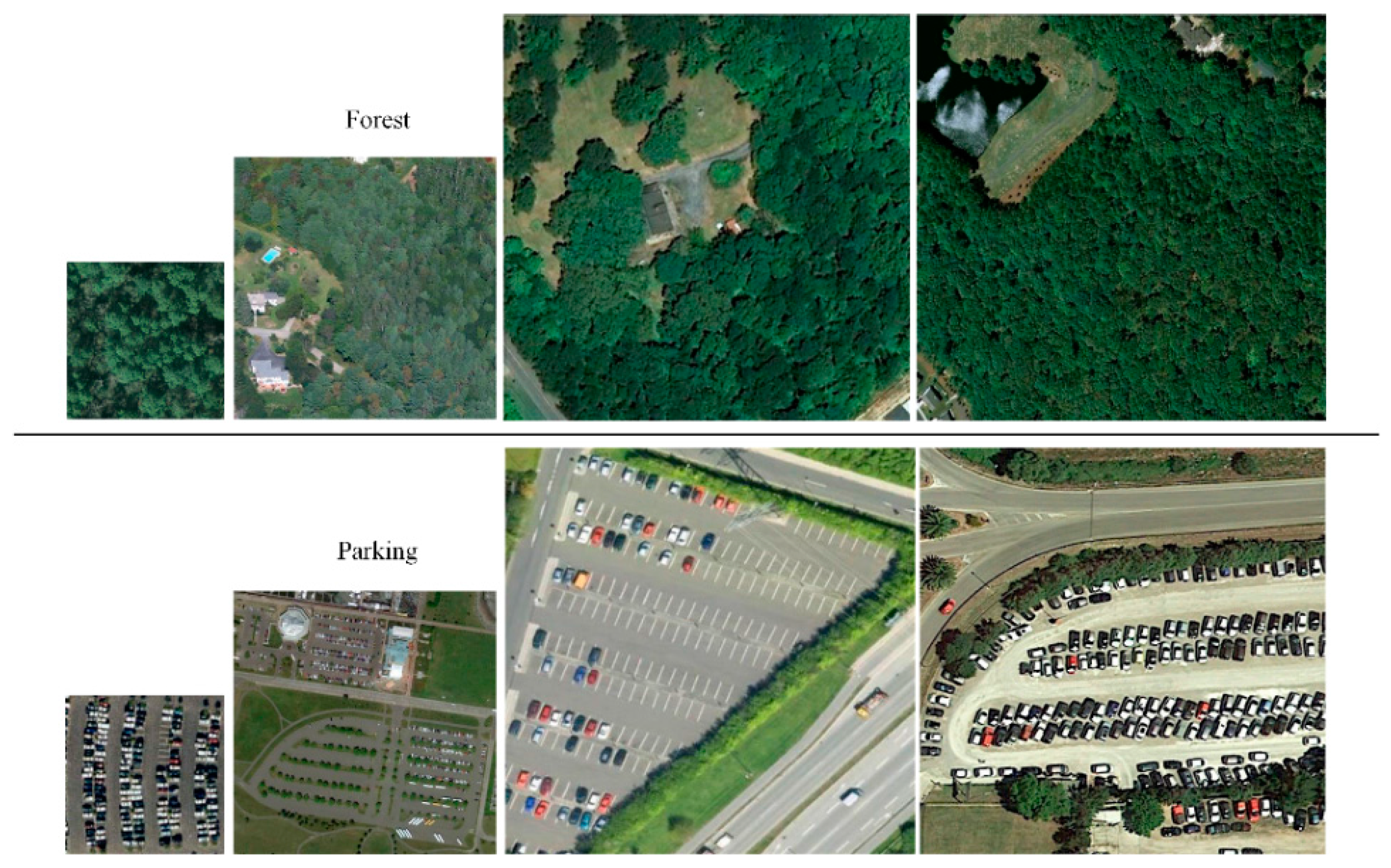
The proposed LDCNN results in a 30-D dimensional feature vector which is very compact compared to deep features extracted by the pre-trained and fine-tuned CNNs. The pre-trained CNN that achieves the best performance in terms of Fc features on each dataset is selected and fine-tuned.

Table 10. Results of the pre-trained CNN, the fine-tuned CNN, and the proposed LDCNN on the UCMD, RSD, and RSSCN7 datasets. For the pre-trained CNN, we choose the best results, as shown in Table 6 and Table 7; for the fine-tuned CNN, VGGM, CaffeRef, and VGGS are fine-tuned on AID and then applied to UCMD, RSD, and RSSCN7, respectively. The numbers are ANMRR values.

Datasets	Pre-Trained CNN	Fine-Tuned CNN				LDCNN
		Fc1	Fc1_ReLU	Fc2	Fc2_ReLU
UCMD	0.375	0.349	0.334	0.329	0.340	0.439
RSD	0.279	0.185	0.062	0.044	0.036	0.019
RSSCN7	0.388	0.361	0.337	0.304	0.312	0.305

shows the results of the fine-tuned CNNs and the proposed LDCNN on these three benchmark datasets. We can see the proposed LDCNN greatly improves the best results of the pre-trained CNNs on RSD and RSSCN7 datasets by 26% and 8.3%, respectively, and the performance is even better than that of the fine-tuned Fc features. However, LDCNN performs worse than the pre-trained and the fine-tuned CNNs on UCMD dataset. These results make sense because LDCNN is trained on the AID dataset which is quite different from the UCMD dataset but similar to the other two datasets and in particular the RSD dataset, in terms of image size and spatial resolution. Figure 11 shows some example images of the same class taken from the four datasets. It is evident that the images of UCMD are at a different scale level with respect to the images of AID dataset, while the images of RSD and RSSCN7 (especially RSD) are similar to that of AID dataset. In addition, we can see the fine-tuned CNN only achieves slightly better performance than the pre-trained CNN on UCMD dataset, which also indicates that the worse performance of LDCNN on UCMD is due to the differences between the UCMD and AID datasets.

Figure 12 shows the number of parameters (weights and biases) contained in the mlpconv layer of LDCNN and in the three Fc layers of the pre-trained and fine-tuned CNNs. It is observed that LDCNN has about 2.6 times fewer parameters than the fine-tuned CNNs and 2.7 times fewer parameters than the pre-trained CNNs. This results in LDCNN being significantly easier to train than the other approaches.

5. Discussion

From the extensive experiments, the two proposed schemes were proven to be effective methods for HRRSIR. Some practical observations from the experiments are summarized as follows:

• The deep feature representations extracted by the pre-trained CNNs, the fine-tuned CNNs, and the proposed LDCNN achieved superior performance to state-of-the-art hand-crafted features. The results indicate that CNN can generate powerful feature representations for HRRSIR.
• In the first scheme, the pre-trained CNNs were regarded as feature extractors to extract Fc and Conv features without any labelled images. Fc features can be directly extracted from Fc1 and Fc2 layers, while feature aggregation methods (BOVW, VLAD, and IFK) are needed in order to utilize Conv features. To give an extensive evaluation of the deep features, we investigated the effect of ReLU on Fc and Conv features. The results show that Fc1 features achieved better performance than Fc2 feature without the use of ReLU but achieved worse performance with the use of ReLU, indicating that nonlinearity improves retrieval performance if the features are extracted from higher layers. Regarding the Conv features, it is interesting that the use of ReLU decreased the performance of Conv features on the benchmark datasets except for the UCMD dataset. A possible explanation is that these existing feature aggregation methods are designed for traditional hand-crafted features which have quite different distributions of pairwise similarities from deep features [20].
• In the second scheme, we proposed two approaches to further improve the performance of the pre-trained CNNs with limited labelled images. The first approach was fine-tuning the pre-trained CNNs on the target remote sensing dataset to learn domain-specific features. While for the second approach, a novel CNN that can learn low dimensional features for HRRSIR was proposed based on conventional convolution layers and a three-layer perceptron. In order to speed up training, the parameters of the convolution layers were transferred from VGGM. The proposed LDCNN was able to generate 30-D dimensional feature vectors which are more compact than the Fc and Conv features. As shown in Table 10, LDCNN outperformed the pre-trained CNNs and the fine-tuned CNNs on the RSD and RSSCN7 datasets but achieved worse performance on the UCMD dataset. This is because the images in UCMD and AID are quite different in terms of image size and spatial resolution. LDCNN provides a direction for us to directly learn low dimensional features from CNN which can achieve remarkable performance.
• LDCNN was trained on the AID dataset and then applied to three new remote sensing datasets (UCMD, RSD, and RSSCN7). The remarkable performances on RSD and RSSCN7 datasets indicate that CNN has strong transferability. However, the performance should be further improved if LDCNN is trained on the target dataset. To this end, a much larger dataset needs to be constructed.

6. Conclusions

We presented two effective schemes to extract deep feature representations for HRRSIR. In the first scheme, the features were extracted from the fully-connected and convolutional layers of a pre-trained CNN, respectively. The Fc features could be directly used for similarity measure, while the Conv features were encoded by feature aggregation methods to generate compact feature vectors before similarity measure. We also investigated the effect of ReLU on Fc and Conv features.

Though the first scheme was able to achieve better performance than traditional hand-crafted features, the pre-trained CNN models were trained on ImageNet, which is quite different from remote sensing datasets. Fine-tuning the pre-trained CNNs on the target dataset is a common strategy to improve the performance of the pre-trained CNNs, however, the features extracted from the fine-tuned Fc layers are 4096-D feature vectors, which are of high dimension for large-scale image retrieval. Thus, we propose a novel CNN architecture based on conventional convolution layers and a three-layer perceptron which is then trained on a large remote sensing dataset. The proposed LDCNN is able to generate 30-D features that can achieve remarkable performance on several remote sensing datasets.

While LDCNN is designed for HRRSIR, it can also be applied to other remote sensing tasks such as scene classification and object detection.

References

- Bretschneider, T.; Cavet, R.; Kao, O. Retrieval of remotely sensed imagery using spectral information content. In Proceedings of the IEEE International Geoscience & Remote Sensing Symposium, Toronto, ON, Canada, 24–28 June 2002; pp. 2253–2255. [Google Scholar]
- Scott, G.J.; Klaric, M.N.; Davis, C.H.; Shyu, C.R. Entropy-balanced bitmap tree for shape-based object retrieval from large-scale satellite imagery databases. IEEE Trans. Geosci. Remote Sens. 2011, 49, 1603–1616. [Google Scholar] [CrossRef]
- Shao, Z.; Zhou, W.; Zhang, L.; Hou, J. Improved color texture descriptors for remote sensing image retrieval. J. Appl. Remote Sens. 2014, 8, 83584. [Google Scholar] [CrossRef]
- Zhu, X.; Shao, Z. Using no-parameter statistic features for texture image retrieval. Sens. Rev. 2011, 31, 144–153. [Google Scholar] [CrossRef]
- Aptoula, E. Remote sensing image retrieval with global morphological texture descriptors. IEEE Trans. Geosci. Remote Sens. 2014, 52, 3023–3034. [Google Scholar] [CrossRef]
- Goncalves, H.; Corte-Real, L.; Goncalves, J.A. Automatic image registration through image segmentation and SIFT. IEEE Trans. Geosci. Remote Sens. 2011, 49, 2589–2600. [Google Scholar] [CrossRef]
- Sedaghat, A.; Mokhtarzade, M.; Ebadi, H. Uniform robust scale-invariant feature matching for optical remote sensing images. IEEE Trans. Geosci. Remote Sens. 2011, 49, 4516–4527. [Google Scholar] [CrossRef]
- Sirmacek, B.; Unsalan, C. Urban area detection using local feature points and spatial voting. IEEE Geosci. Remote Sens. Lett. 2010, 7, 146–150. [Google Scholar] [CrossRef]
- Yang, Y.; Newsam, S. Geographic image retrieval using local invariant features. IEEE Trans. Geosci. Remote Sens. 2013, 51, 818–832. [Google Scholar] [CrossRef]
- LeCun, Y.; Bengio, Y.; Geoffrey, H. Deep learning. Nature 2015, 521, 436–444. [Google Scholar] [CrossRef] [PubMed]
- Wan, J.; Wang, D.; Hoi, S.C.H.; Wu, P.; Zhu, J.; Zhang, Y.; Li, J. Deep learning for content-based image retrieval: A comprehensive study. In Proceedings of the 22nd ACM International Conference on Multimedia, Orlando, FL, USA, 3–7 November 2014; pp. 157–166. [Google Scholar]
- Cheriyadat, A.M. Unsupervised feature learning for aerial scene classification. IEEE Trans. Geosci. Remote Sens. 2014, 52, 439–451. [Google Scholar] [CrossRef]
- Zhou, W.; Shao, Z.; Diao, C.; Cheng, Q. High-resolution remote-sensing imagery retrieval using sparse features by auto-encoder. Remote Sens. Lett. 2015, 6, 775–783. [Google Scholar] [CrossRef]
- Li, Y.; Zhang, Y.; Tao, C.; Zhu, H. Content-Based high-resolution remote sensing image retrieval via unsupervised feature learning and collaborative affinity metric fusion. Remote Sens. 2016, 8, 709. [Google Scholar] [CrossRef]
- Deng, J.; Dong, W.; Socher, R.; Li, L.J.; Li, K.; Fei-Fei, L. ImageNet: A large-scale hierarchical image database. In Proceedings of the 2009 IEEE Conference on Computer Vision and Pattern Recognition, Miami, FL, USA, 20–26 June 2009; pp. 2–9. [Google Scholar]
- Marmanis, D.; Datcu, M.; Esch, T.; Stilla, U. Deep Learning earth observation classification using Imagenet Pretrained Networks. IEEE Geosci. Remote Sens. Lett. 2015, 13, 1–5. [Google Scholar] [CrossRef]
- Penatti, O.A.B.; Nogueira, K.; Dos Santos, J.A. Do deep features generalize from everyday objects to remote sensing and aerial scenes domains? In Proceedings of the IEEE Computer Society Conference on Computer Vision and Pattern Recognition Workshops, Boston, MA, USA, 7–12 June 2015. [Google Scholar]
- Castelluccio, M.; Poggi, G.; Sansone, C.; Verdoliva, L. Land use classification in remote sensing images by convolutional neural networks. arXiv, 2015; arXiv:1508.00092. [Google Scholar]
- Chandrasekhar, V.; Lin, J.; Morère, O.; Goh, H.; Veillard, A. A practical guide to CNNs and Fisher Vectors for image instance retrieval. Signal Process. 2016, 128, 426–439. [Google Scholar] [CrossRef]
- Yandex, A.B.; Lempitsky, V. Aggregating local deep features for image retrieval. In Proceedings of the IEEE International Conference on Computer Vision, Santiago, Chile, 7–13 December 2015; pp. 1269–1277. [Google Scholar]
- Stutz, D. Neural Codes for Image Retrieval. In Proceedings of the Computer Vision—ECCV 2014, Zurich, Switzerland, 6–12 September 2014; pp. 584–599. [Google Scholar]
- Napoletano, P. Visual descriptors for content-based retrieval of remote sensing images. arXiv, 2016; arXiv:1602.00970. [Google Scholar]
- Nanni, L.; Ghidoni, S. How could a subcellular image, or a painting by Van Gogh, be similar to a great white shark or to a pizza? Pattern Recognit. Lett. 2017, 85, 1–7. [Google Scholar] [CrossRef]
- Xu, B.; Wang, N.; Chen, T.; Li, M. Empirical evaluation of rectified activations in convolution network. arXiv, 2015; arXiv:1505.00853. [Google Scholar]
- Glorot, X.; Bordes, A.; Bengio, Y. Deep sparse rectifier neural networks. In Proceedings of the 14th International Conference on Artificial Intelligence and Statistics (AISTATS’11), Fort Lauderdale, FL, USA, 11–13 April 2011; pp. 315–323. [Google Scholar]
- Krizhevsky, A.; Sutskever, I.; Hinton, G.E. ImageNet classification with deep convolutional neural networks. Adv. Neural Inf. Process. Syst. 2012, 25, 1–9. [Google Scholar]
- Jia, Y.; Shelhamer, E.; Donahue, J.; Karayev, S.; Long, J.; Girshick, R.; Guadarrama, S.; Darrell, T. Caffe: Convolutional Architecture for Fast Feature Embedding. In Proceedings of the ACM International Conference on Multimedia, Orlando, FL, USA, 3–7 November 2014; pp. 675–678. [Google Scholar]
- Chatfield, K.; Chatfield, K.; Simonyan, K.; Vedaldi, A.; Zisserman, A. Return of the devil in the details: Delving deep into convolutional nets. In Proceedings of the British Machine Vision Conference, Nottinghamshire, UK, 1–5 September 2014; pp. 1–11. [Google Scholar]
- Simonyan, K.; Zisserman, A. Very deep convolutional networks for large-scale image recognition. arXiv, 2014; arXiv:1409.1556. [Google Scholar]
- Hinton, G.E.; Srivastava, N.; Krizhevsky, A.; Sutskever, I.; Salakhutdinov, R.R. Improving neural networks by preventing co-adaptation of feature detectors. arXiv, 2012; arXiv:1207.0580. [Google Scholar]
- Vedaldi, A.; Lenc, K. MatConvNet. In Proceedings of the 23rd ACM International Conference on Multimedia, Brisbane, Australia, 26–30 October 2015; pp. 689–692. [Google Scholar]
- Özkan, S.; Ateş, T.; Tola, E.; Soysal, M.; Esen, E. Performance analysis of state-of-the-art representation methods for geographical image retrieval and categorization. IEEE Geosci. Remote Sens. Lett. 2014, 11, 1996–2000. [Google Scholar] [CrossRef]
- Gong, Y.; Wang, L.; Guo, R.; Lazebnik, S. Multi-scale orderless pooling of deep convolutional activation features. In Proceedings of the European Conference on Computer Vision, Zurich, Switzerland, 6–12 September 2014; pp. 392–407. [Google Scholar]
- Ng, J.Y.; Yang, F.; Davis, L.S. Exploiting Local Features from Deep Networks for Image Retrieval. In Proceedings of the IEEE Conference on Computer Vision and Pattern Recognition Workshops, Boston, MA, USA, 7–12 June 2015; pp. 53–61. [Google Scholar]
- Sivic, J.; Zisserman, A. Video Google: A text retrieval approach to object matching in videos. In Proceedings of the Ninth IEEE International Conference on Computer Vision, Nice, France, 13–16 October 2003; pp. 1470–1477. [Google Scholar]
- Jégou, H.; Douze, M.; Schmid, C.; Pérez, P. Aggregating local descriptors into a compact representation. In Proceedings of the IEEE Conference on Computer Vision & Pattern Recognition, San Francisco, CA, USA, 13–18 June 2010; pp. 3304–3311. [Google Scholar]
- Perronnin, F.; Sánchez, J.; Mensink, T. Improving the Fisher Kernel for Large-Scale Image Classification. In Proceedings of the European Conference on Computer Vision, Heraklion, Greece, 5–11 September 2010; pp. 143–156. [Google Scholar]
- Lin, M.; Chen, Q.; Yan, S. Network in Network. arXiv, 2014; arXiv:1312.4400. [Google Scholar]
- Xia, G.-S.; Yang, W.; Delon, J.; Gousseau, Y.; Sun, H.; Maître, H. Structural high-resolution satellite image indexing. In Proceedings of the ISPRS TC VII Symposium-100 Years ISPRS, Vienna, Austria, 5–7 July 2010; pp. 298–303. [Google Scholar]
- Zou, Q.; Ni, L.; Zhang, T.; Wang, Q. Deep learning based feature selection for remote sensing scene classification. IEEE Geosci. Remote Sens. Lett. 2015, 12, 2321–2325. [Google Scholar] [CrossRef]
- Xia, G.-S.; Hu, J.; Hu, F.; Shi, B.; Bai, X.; Zhong, Y.; Zhang, L. AID: A Benchmark dataset for performance evaluation of aerial scene classification. arXiv, 2016; arXiv:1608.05167. [Google Scholar]
- Ojala, T.; Pietikainen, M.; Maenpaa, T. Multiresolution gray-scale and rotation invariant texture classification with local binary patterns. IEEE Trans. Pattern Anal. Mach. Intell. 2002, 24, 971–987. [Google Scholar] [CrossRef]
- Oliva, A.; Torralba, A. Modeling the shape of the scene: A holistic representation of the spatial envelope. Int. J. Comput. Vis. 2001, 42, 145–175. [Google Scholar] [CrossRef]
- Cheng, G.; Han, J.; Lu, X. Remote Sensing Image Scene Classification: Benchmark and State of the Art. arXiv, 2017; arXiv:1703.00121. [Google Scholar]
- Lowe, D.G. Distinctive image features from scale-invariant keypoints. Int. J. Comput. Vis. 2004, 60, 91–110. [Google Scholar] [CrossRef]
Figure 1.
The typical architecture of convolutional neural networks (CNNs). The rectified linear units (ReLU) layers are ignored here for conciseness.
Figure 2.
Flowchart of the first scheme: deep features extracted from Fc2 and Conv5 layers of the pre-trained CNN model. For conciseness, we refer to features extracted from Fc1–2 and Conv1–5 layers as Fc features (Fc1, Fc2) and Conv features (Conv1, Conv2, Conv3, Conv4, Conv5), respectively.
Figure 3.
Flowchart of extracting features from the fine-tuned layers. Dropout1 and dropout2 are dropout layers which are used to control overfitting. N is the number of image classes in the target dataset.
Figure 4.
The overall structure of the proposed, novel CNN architecture. There are five linear convolution layers and an mlpconv layer followed by a global average pooling layer.
Figure 5.
Sample images from the University of California, Merced dataset (UCMD) dataset. From the top left to bottom right: agricultural, airplane, baseball diamond, beach, buildings, chaparral, dense residential, forest, freeway, golf course, harbor, intersection, medium density residential, mobile home park, overpass, parking lot, river, runway, sparse residential, storage tanks, and tennis courts.
Figure 6.
Sample images from the remote sensing dataset (RSD). From the top left to bottom right: airport, beach, bridge, commercial area, desert, farmland, football field, forest, industrial area, meadow, mountain, park, parking, pond, port, railway station, residential area, river, and viaduct.
Figure 7.
Sample images from the RSSCN7 dataset. From left to right: grass, field, industry, lake, resident, and parking.
Figure 8.
Samples images from the aerial image dataset (AID). From the top left to bottom right: airport, bare land, baseball field, beach, bridge, center, church, commercial, dense residential, desert, farmland, forest, industrial, meadow, medium residential, mountain, park, parking, playground, pond, port, railway station, resort, river, school, sparse residential, square, stadium, storage tanks, and viaduct.
Figure 9.
The effect of ReLU on Fc1 and Fc2 features. (a) Results on UCMD dataset; (b) Results on RSD dataset; (c) Results on RSSCN7 dataset; (d) Results on AID dataset. For Fc1_ReLU and Fc2_ReLU features, ReLU is applied to the extracted Fc features.
Figure 10.
The effect of ReLU on Conv features. (a) Results on UCMD dataset; (b) Results on RSD dataset; (c) Results on RSSCN7 dataset; (d) Results on AID dataset. For BOVW_ReLU, VLAD_ReLU, and IFK_ReLU features, ReLU is applied to the Conv features before feature aggregation.
Figure 11.
Comparison between images of the same class from the four datasets. From left to right, the images are from UCMD, RSSCN7, RSD, and AID respectively.
Figure 12.
The number of parameters contained in VGGM, fine-tuned VGGM, and LDCNN.