Flood Inundation Mapping from Optical Satellite Images Using Spatiotemporal Context Learning and Modest AdaBoost

Abstract

Due to its capacity for temporal and spatial coverage, remote sensing has emerged as a powerful tool for mapping inundation. Many methods have been applied effectively in remote sensing flood analysis. Generally, supervised methods can achieve better precision than unsupervised. However, human intervention makes its results subjective and difficult to obtain automatically, which is important for disaster response. In this work, we propose a novel procedure combining spatiotemporal context learning method and Modest AdaBoost classifier, which aims to extract inundation in an automatic and accurate way. First, the context model was built with images to calculate the confidence value of each pixel, which represents the probability of the pixel remaining unchanged. Then, the pixels with the highest probabilities, which we define as ‘permanent pixels’, were used as samples to train the Modest AdaBoost classifier. By applying the strong classifier to the target scene, an inundation map can be obtained. The proposed procedure is validated using two flood cases with different sensors, HJ-1A CCD and GF-4 PMS. Qualitative and quantitative evaluation results showed that the proposed procedure can achieve accurate and robust mapping results.

1. Introduction

Natural disasters are common phenomena in all parts of the world. There are many types of natural disasters [1], of which a flood is considered to be one of the most destructive, widespread and frequent disasters [2,3]. Every year, tremendous loss of life and property is caused by flooding [3]. Due to the changes in global climate and land use, floods are becoming more severe and more frequent all around the world [3,4]. Although it is difficult to prevent floods, it is possible to minimise their impact through proper rescue, relief and resource allocation for recovery and reconstruction. Therefore, accurate inundation mapping, especially near real time, is very important for establishing a fast response plan and mitigating the disaster [5,6,7].

Traditional methods for inundation mapping are based on ground survey and aerial observation. However, when the flood spreads to a large scale, these approaches are time- and resource-consuming, which cannot satisfy the need for a fast response to a disaster. Moreover, aerial observation can be unrealistic in some extreme weather conditions, and the density of gauging stations is not satisfactory in many countries [8]. An alternative choice is provided by satellite remote sensing (RS) techniques [6]. Due to their time availability and cost effectiveness, satellite data has played an important role in understanding inundation [9,10,11,12,13]. The availability of multi-date images makes it possible to monitor the progress of floods.

Satellites used for mapping floods can be divided into those that are optical and those that are microwave. Due to its capacity to penetrate the frequent clouds in a flood event, microwave remote sensing is all-weather and invaluable for flood monitoring. With multispectral images, the flood can be analysed in a more straightforward way with simpler pre-processing [14]. In this study, we mainly focus on methods using multispectral satellite images.

Numerous methods have been proposed for mapping inundation using multispectral remote sensing images. Among them, the one most frequently used is thresholding. Usually, indices are first calculated through different band combinations, such as the normalised difference water index (NDWI) created by McFeeters [15], which has been proven to produce good results for inundated areas [16]. Then a threshold is selected to determine the water range in the image. A manual threshold is accurate, but has difficulty satisfying the need for fast disaster response. Moreover, it is subjective, as different operators may produce different results. To overcome the problems, unsupervised thresholding methods have been proposed. For instance, Xie et al. [17] introduced Otsu’s algorithm to implement automatic selection of the water threshold. But due to the common illumination differences and mixed pixels in satellite images, its effectiveness is reduced, especially for some complicated scenes.

The segmentation (semi-supervised) technique [18] has been proposed to minimise the involvement of the user. The user first selects some seed points, with which the connectivity map is generated using fuzzy logic. For example, in [19], a fast flood map and a detailed flood map were obtained using growing strategies with seed points. However, the detailed map result still depended on the correctness of the seed points.

Unsupervised strategies without any human involvement have attracted a lot of attention in recent years. There are several kinds of unsupervised inundation mapping methods. Besides the unsupervised threshold, unsupervised feature extraction methods have been utilised. Chignell et al. [20] combines the pre- and post-flood images and apply the independent component analysis (ICA) to them. Segmentation and threshold are used to extract the flood from the change components. The cloud and crop components help to refine the maximum flood extent. In the work by Rokni et al. [21], the multi-temporal NDWI images are composited into one file. Principal component analysis (PCA) is applied to the composited file. The principle components are classified by the thresholding technique, and the result of the change detection for the lake is obtained. But these methods are only based on spectral information. When they are applied to cases using different sensors, the ability of the method can vary with the changes of spectral characteristics.

Recently, context information, especially spatiotemporal context information, has attracted more attention and proven to bring much improvement in monitoring the water surface. It is combined with other techniques to generate chains of processing for better representation of an event. Chen et al. [22] proposed a water surface monitoring method using contextual information. First, permanent water/non-water pixels were detected by judging the statistical consistency between an image point and its neighbourhood. Then, a distance-based classifier was used to map the other pixels with the obtained permanent pixels. Experiments on Moderate Resolution Imaging Spectroradiometer (MODIS) proved its validity and superiority over other unsupervised methods. However, the proposed definition of the statistical equality depended on simple one-dimensional features, which were the means and mediums of temporally adjacent pixels. A pixel was considered to be permanent if it had more than five spatially adjacent and statistically equal pixels. This simple count strategy can reduce the robustness of the method. Moreover, the low spatial resolution of MODIS data also limited its performance in spatial dimension.

To resolve these issues, in this paper, we introduce a spatiotemporal context learning (STCL) method and propose a novel work flow for flood mapping. The main objective is to delineate the water surface in an accurate and automatic way. First, a statistical model is built for the contextual information of multi-temporal NDWI. Then, permanent pixels are extracted according to their contextual consistency confidence values calculated from the model. Finally, a Modest AdaBoost (MADB) classifier, trained with the permanent pixels and a variety of spectral characteristics, is adopted to map the image into water and non-water categories. Through making full use of the spatiotemporal and spectral information, the proposed approach improves the ability to map inundated surfaces. The uncertainty caused by the sensor and scene differences is also reduced. Two different multispectral datasets with medium resolution, HJ-1A CCD (30 m) and GF-4 PMS (50 m), are employed for the validation.

2. Experimental Set Up

2.1. Datasets

Several kinds of multispectral satellite data have been used for flood mapping, such as Advanced Very High Resolution Radiometer (AVHRR), MODIS, and Landsat TM/ETM+ data. However, most of these data do not have high spatial and temporal resolution at the same time [23]. This has limited their ability to map inundation, which changes complicatedly and rapidly over time. For example, AVHRR and MODIS have a frequent revisiting cycle, which can be even shorter than 1 day. Their high temporal resolution makes them useful for monitoring environmental changes, while the spatial resolution of AVHRR and MODIS is 1 km and 250 m, respectively, which is coarse. Only general extent, not accurate results, can be obtained using these data for flood mapping. On the contrary, Landsat TM/ETM+ data have a middle-to-high spatial resolution of 30 m, but the observation is repeated every 16 days, which cannot satisfy the needs for timely response.

On 6 September 2008, two optical satellites named HJ-1A/B (short for HuanJing-1A/B), also known as the Chinese Environment and Disaster Monitoring and Forecasting Small Satellite Constellation, were launched in China. The data can be downloaded from the website (http://www.cresda.com/) free of charge, and have been successfully applied in several applications such as land mapping, yield prediction, and environment assessment. The two satellites were equipped with CCD cameras, which take multispectral images on the earth surface with a spatial resolution of 30 m. For each satellite, the time interval is 4 days. The constellation of the two satellites theoretically has a higher revisiting frequency of 2 days. With both the advantages of spatial and temporal resolution, HJ-1A/B satellites are regarded as an effective tool for monitoring and post-flood assessment [24].

The recently emerged geostationary satellite GaoFen-4 (GF-4) also has a high application value in rapid assessment and emergency response of floods [25]. Due to its optical geostationary orbit, GF-4 shows a better performance in time resolution over other satellites. It is equipped with a camera for visible, near infrared and middle-wavelength infrared spectra. The spatial resolution is 50 m. To the best of our knowledge, research work using GF-4 imagery is limited, as it was only launched on 29 December 2015, and officially put in use on 13 June 2016. In this work, we also want to explore the potential of the multispectral GF-4 PMS data in flood mapping. The main parameters of the HJ-1A/B CCD data and GF-4 PMS data are listed in

Table 1. Technical parameters of the HJ-1A/B CCD data.

Satellite Sensor	Band No.	Spectral Range (µm)	Spatial Resolution (m)	Revisiting Time
HJ-1A/B CCD	1	0.43–0.52	30	4 days
	2	0.52–0.60
	3	0.63–0.69
	4	0.76–0.90

and

Table 2. Technical parameters of the GF-4 PMS data.

Satellite Sensor	Band No.	Spectral Range (µm)	Spatial Resolution (m)	Revisiting Time
GF-4 PMS	1	0.45–0.90	50	20 s
	2	0.45–0.52
	3	0.52–0.60
	4	0.63–0.69
	5	0.76–0.90

. Slightly different from the HJ-1A/B CCD data, the GF-4 PMS data have an additional panchromatic band.

As can be seen, the HJ-1A/B CCD data and the GF-4 PMS data show balanced abilities in spatial and temporal resolutions. Due to the limitations stated above in other multispectral data, we decide to utilise these two datasets for verifying the methods, and for understanding more about the potential of these two datasets in flood mapping as well, as they are not so commonly used as MODIS or Landsat data. Certainly, another reason why the HJ-1A/B CCD and GF-4 PMS data are chosen is because of their free access.

2.2. Study Area

The Heilongjiang River is one of the largest rivers in Northeast Asia, flowing through four countries (Mongolia, China, Russia and North Korea). The main stream has a total length of 2821 km, and also forms the boundary between China and Russia. There are abundant water resources in the Heilongjiang River, with a yearly runoff of 346.5 billion cubic meters. The main climate type in that region is monsoon. The precipitation distribution varies with the season. From April to October, the precipitation accounts for 90–93% of the annual precipitation, and the period from June to August accounts for 60–70%. From December, the winter dry season starts and the precipitation mainly falls in the form of snow.

From 12 August 2013, several severe precipitation events continuously hit the northeastern part of Asia, leading to great flood in 39 rivers including part of the Heilongjiang River. Especially for the Tongjiang and Fuyuan Reaches of the Heilongjiang River, the flood had been the most serious one in the past 100 years. On 24 August 2013, more than 5 million people were affected in this disaster. The first case study analyses the event in this region. Two cloud-free scenes of HJ-1A CCD data are utilised. One image was obtained on 12 July 2013, which is around one month before the flood, and the other one was obtained on 27 August 2013 during the peak flow period. The dimension of the study region is 1082 × 1321 pixels (around 1286 square kilometres). Its location and extent are shown in Figure 1.

Dongting Lake is one of the most essential lakes in China, and one of the most important wetlands in the world as well. It is located on the southern bank of the Jinjiang section of the middle Yangtze River, and is one of the important dispatching lakes for the Yangtze River because of the strong ability of flood storage. The area of the lake is approximately 2690 square kilometres, across Hunan and Hubei provinces, and is roughly composed of East Dongting Lake, South Dongting Lake and West Dongting Lake. The water of Dongting Lake is clean and this area is one of the main freshwater fishery bases for commercial purposes. Due to its good environment and richness in water, soil and wildlife resources, it is one of the earliest birth places of Chinese rice raising agriculture. The basin area is of 262.8 thousand square kilometres, accounting for 14.6% of the Yangtze River basin area.

In June and July 2016, heavy rains hit the middle and lower reaches of the Yangtze River basin, causing a catastrophic and wide flood in southern China. Eleven provinces and more than 10 million people were affected. On 3 July 2016, the water at the Chenglingji station in Dongting Lake also surpassed the warning level 32.50 m. A regional flood occurred in Dongting Lake. The second case study focuses on this area during this flood. Two cloud-free GF-4 PMS images are selected as the experimental data, which were obtained on 17 June 2016 (before the flood occurred) and 23 July 2016 (during the flood period), with a dimension of 2534 × 2235 pixels (around 14,159 square kilometres). The location and extent of the second study site are shown in Figure 2.

As can be seen from the figures, these two study sites are located in different geographic positions. The first case study mainly presents a river flood and the second one presents a lake flood. Studies on different kinds of floods can help validate the robustness of the method. Moreover, these two floods took place in 2013 and 2016. Each of them is one of the most severe flood events in that year, bringing about a large amount of damage and wide effects. The areas covered by the first and the second case studies are also areas with high flood risk every year, so it is significant to choose these two areas for study, which can help the government to make better decisions in disaster prevention in these areas.

Before the experiment, these two pairs of data are preprocessed. For HJ-1A/B CCD data, we download the absolute calibration coefficients from the data source website (http://www.cresda.com/), and apply the absolute radiometric corrections to the data. These coefficients are obtained through field experiment and authenticity testing by the China Centre for Resource Satellite Data and Application (CRESDA). For the GF-4 PMS data and the GF-1 WFV data used for validation, a relative radiometric correction is implemented before they are archived. We have not made further modifications to their radiation values. All the satellites images used in this study are geometrically registered using the software ERDAS IMAGEINE AutoSync. Specifically, in either of these two case studies, the experimental data before the flood is considered the reference data. Other images used in the same case are all registered to it. The co-registration technology adopts the cubic polynomial. The mean displacement error is 0.5 pixels. All the data are projected to the WGS 1984 UTM coordinate system.

2.3. Validation

The extent of the water surface during a flood process can have daily changes. It is almost impossible to obtain an accurate map of inundation regions on a particular day. In general, most of the flood products are a rough outline of the main inundated areas. In order to achieve the qualitative and quantitative evaluation, we produce two approximate reference maps for the first and second case studies. Either of them is based on a remote sensing image over the same site and taken on the same date as the corresponding experiment data. The spatial resolution of the data used for generating the reference map is necessarily higher than that of the experiment data. For the first case study using HJ-1A/B CCD data, there is a scene of GF-1 WFV data that can meet the requirements. The technical parameters of the GF-1 WFV data are listed in

Table 3. Technical parameters of the GF-1 WFV data.

Satellite Sensor	Band No.	Spectral Range (µm)	Spatial Resolution (m)	Width
GF-1 WFV	1	0.45–0.52	16	800 km
	2	0.52–0.59
	3	0.63–0.69
	4	0.77–0.89

. For the second case using GF-4 PMS data, no corresponding GF-1 WFV data could be found. Instead, we find a scene of HJ-1B CCD data that is qualified. The technical parameters of the HJ-1B CCD data can be found in Table 1.

For the process of how the reference map is made, we use a traditional water extraction method. We take the first case study as an example. First, the selected GF-1 WFV image is geometrically registered to the experimental HJ-1A CCD data. Then, we calculate the NDWI of the GF-1 WFV image. Compared with the ground information from Google Earth software, we manually select a threshold in NDWI to separate water and non-water pixels. Finally, the binary water mask is resampled to the spatial resolution of HJ-1A CCD data (30 m). Similar processes are applied to the second case study. Given that there is no detailed ground truth available, and that it is not feasible to get one by field investigation, we use the reference map in this study as an approximation of the real inundated extent, helping to evaluate and compare the detection results qualitatively and quantitatively.

3. Methods

3.1. Permanent Pixel Extraction Using Spatiotemporal Context Learning

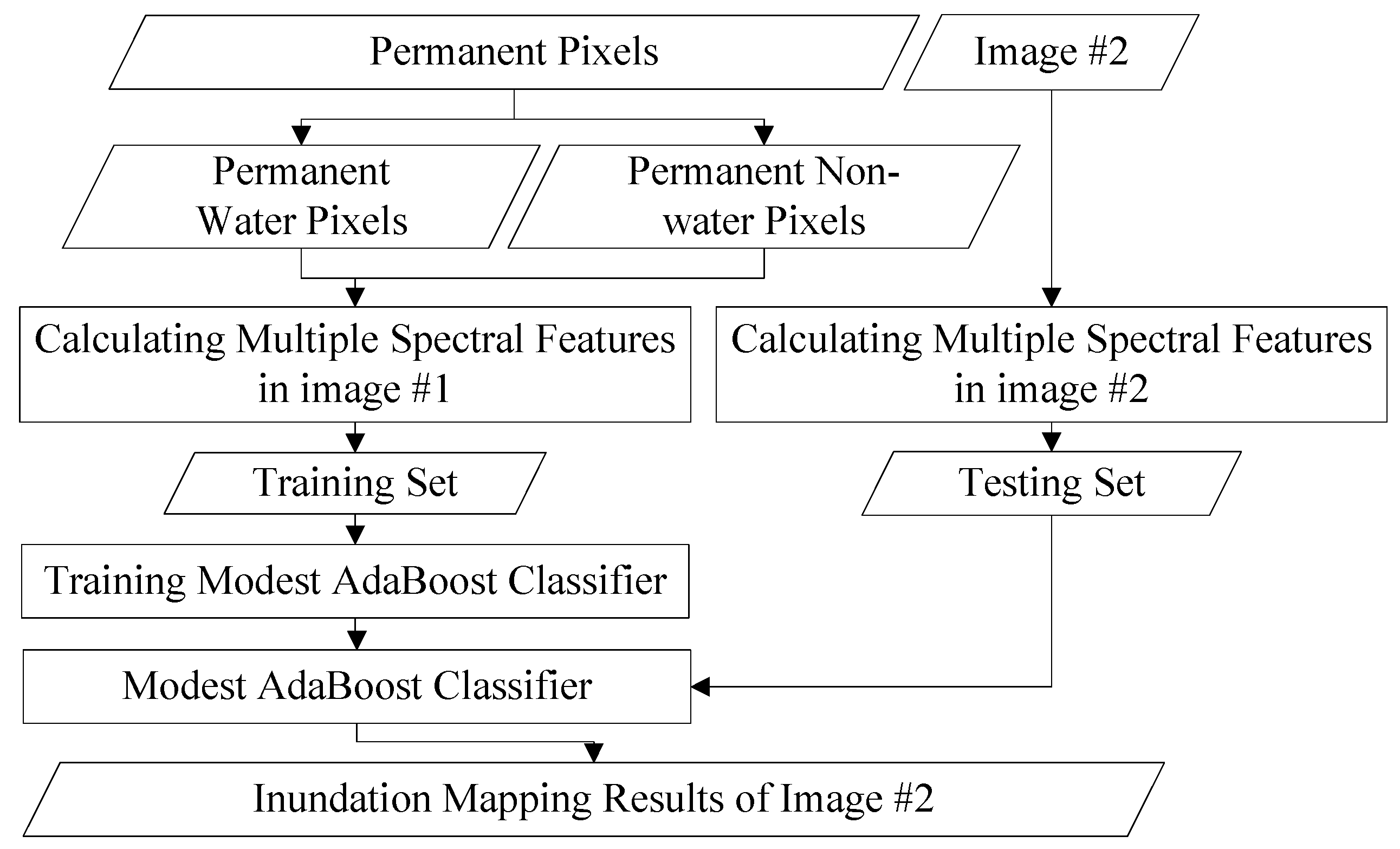
The images before and after a flood are referred to as image #1 and image #2, respectively. The pixels with a constant land cover type, no matter what the type is, are defined as permanent pixels. The proposed method is divided into two steps. First, the permanent pixels in image #1 and image #2 are extracted based on the STCL strategy. This is a method that models the relative relationship between an object and its context. We introduce it to formulate the relationship between a satellite image pixel and its context. Through comparing the models at different time points, a confidence value for whether a pixel changes or not is calculated to extract the permanent pixels. Second, using these permanent pixels as a training set, a widely adopted machine learning classifier, Modest AdaBoost, is trained and implemented for mapping inundation in image #2. Modest AdaBoost is one of the derivations of the boosting algorithm, like the original AdaBoost algorithm. It combines the performance of a set of weak classifiers, and also proves better than other boosting algorithms for convergence ability. More details about these methods will be given below. In this section, we will first discuss the procedure in the first step.

Due to its capacity for targeting specific land cover type and reducing influence from inconstant band representation, spectral indices are commonly used in diverse remote sensing applications, such as disaster monitoring, land cover mapping and disease prevention [26,27,28]. For mapping different cover types in different applications, various indices have been proposed, including the normalised difference vegetation index (NDVI), the enhanced vegetation index (EVI), NDWI, and the normalised difference built-up index (NDBI) and so on. 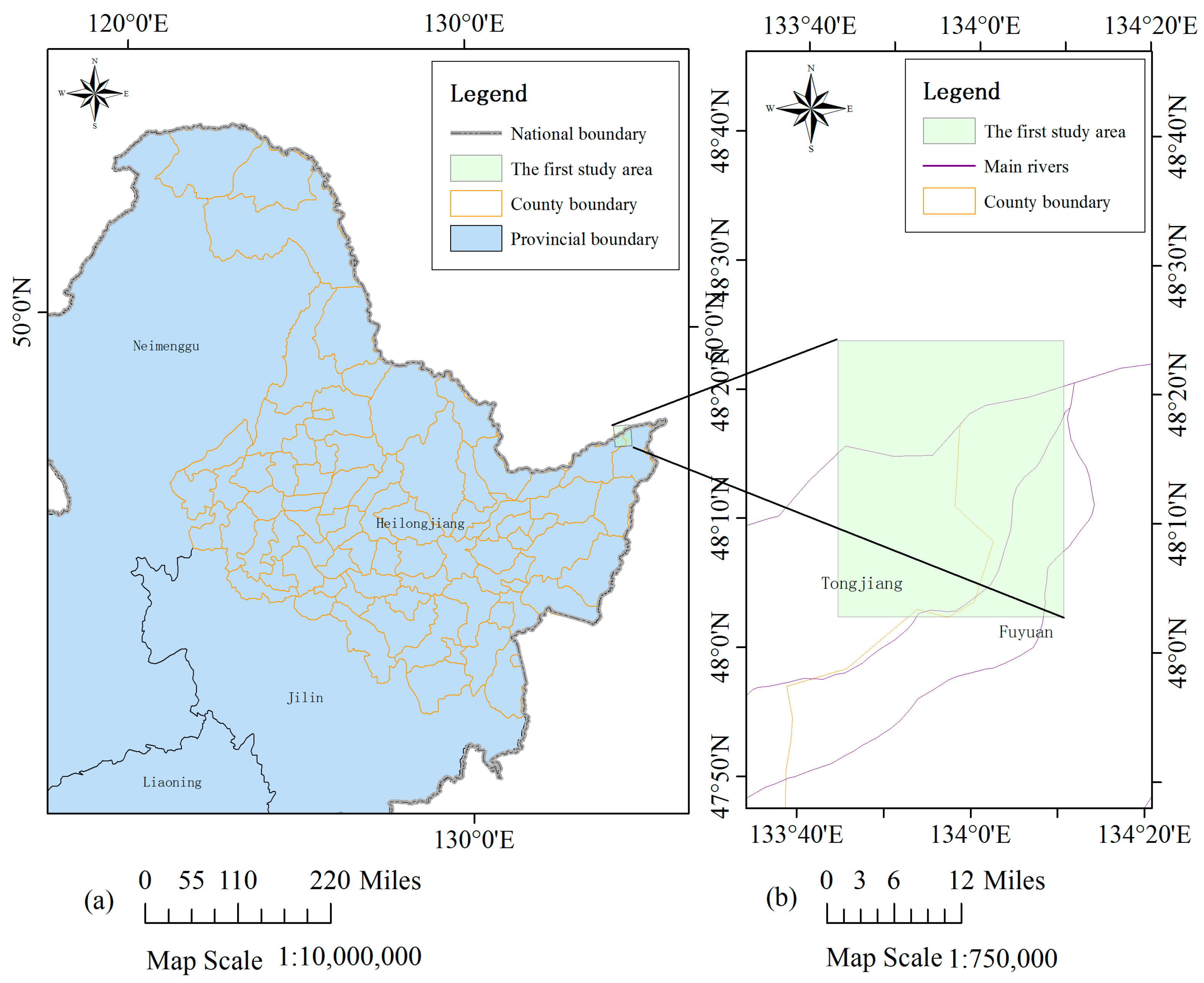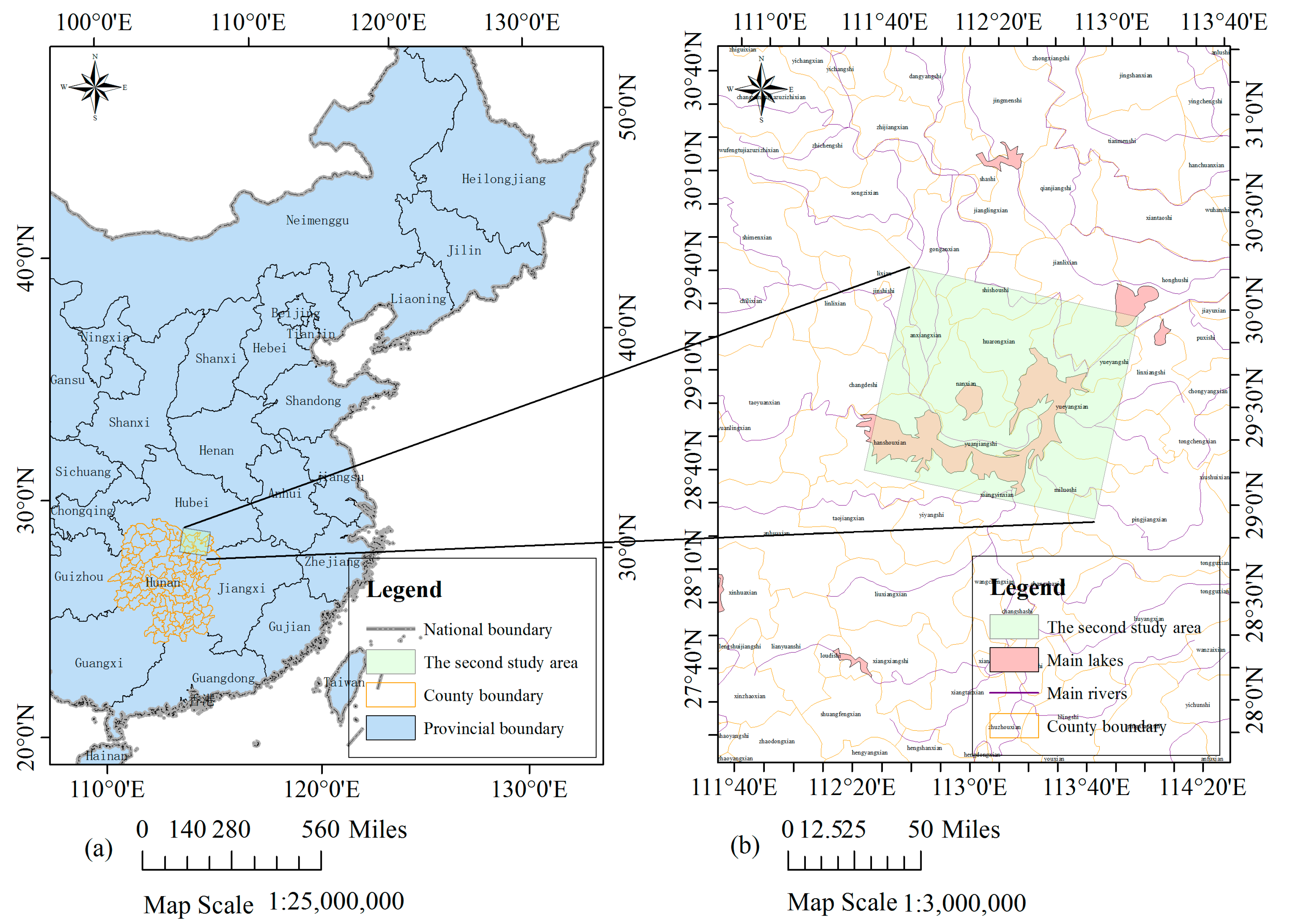Among these indices, the NDWI has been successfully applied to mapping land surface water, and proved more effective than other general feature classification methods [29]. In this study, we calculate the NDWI in the experimental datasets (the HJ-1A CCD data for the first case study and the GF-4 PMS data for the second case study) first. Then, the steps for extracting permanent pixels will be executed on the NDWI data. The NDWI is calculated as:

$$\mathrm{NDWI}=\frac{\mathrm{Green}-\mathrm{NIR}}{\mathrm{Green}+\mathrm{NIR}}$$

(1)

where $\mathrm{Green}$ and $\mathrm{NIR}$ are the reflected green and near infrared radiance, respectively, which are replaced by band 2 and band 4 in the HJ1-A CCD data case, and band 3 and band 5 in the GF-4 PMS data case [15]. NDWI can eliminate the influence from the band value difference, but not the influence caused by the different weather conditions. However, as it is the relative relationship between neighbouring pixels that we use, influences from changes of overall brightness are limited in the proposed procedure.

In the visual tracking field, as the video frames usually change continuously, a strong spatiotemporal correlation is thought to exist between a target and its surroundings. In order to make better use of this relative relationship, Zhang et al. [30] proposed the STCL method. In this method, a rectangular contextual region was first built with the target in the centre. With the low-level features (including the image density and location) of the contextual region, the relative relationship between the target and its surroundings in contextual region was modelled. When a new frame came, it was put into the model to calculate a confidence map, indicating the location that best matched the contextual relationship of previous frames. This location was the inferred location of the target in the new frame. As it depended on a kind of relative relationship, the illumination difference during the frames cannot influence the result. Extensive experiments showed its effectiveness and good degree of precision. This method has also been further employed and extended in other visual trackers [31,32].

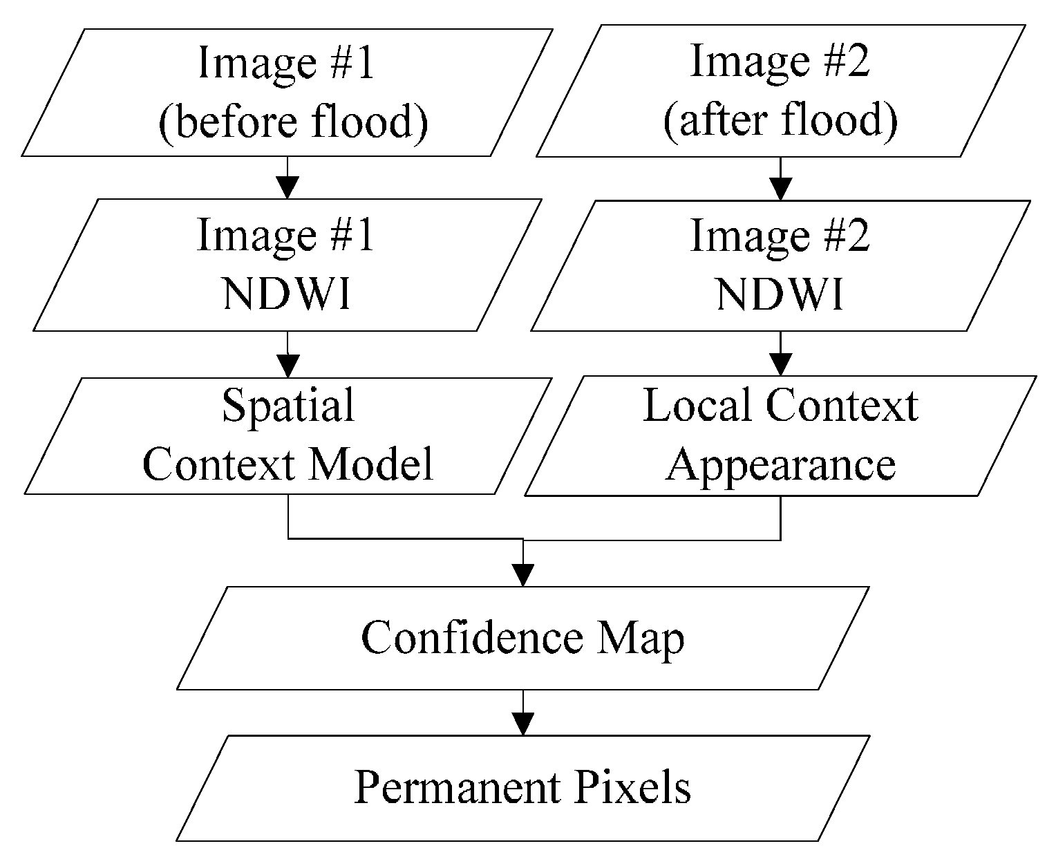
A remote sensing image time series shares many similar characteristics with video data, although video sequence images have a higher sampling rate. It can be inferred that there is also a relationship between a target pixel and its spatiotemporal neighbourhoods in a local scene of RS images, if the images are of good quality, without too many clouds and shadows. Due to the constant changes in weather and light conditions, radiation values of the same cover type can vary greatly in different scenes. Furthermore, it is rather difficult to calibrate the radiation of two RS images to absolute consistency. As a result, more false positives can be introduced in mapping the changes. While the relative relationship between unchanged pixels and their nearby pixels is relatively constant, the STCL method, which aims at modelling this kind of relationship, is supposed to be robust also to illumination variation in RS images. What is more, the STCL method provides a fast solution to online problems. In this work, we borrow the concept of STCL to build a procedure for extracting permanent pixels for flood mapping. The proposed flowchart for extracting permanent pixels is shown in Figure 3.

One core of the STCL method is its utilisation of the attention focus property in biological visual systems. In the mechanism of biological vision, assume that we are observing a point in a picture. Besides the point itself, which draws most of our attention, other points around the target point are the part we pay the second most attention to in the picture. The further one point is from the target point, the less concern it will get from the visual system. On the contrary, if someone tries to find a known point in an image, the visual mechanism first roughly figures out the background of the target, and then, on the basis of a correlation between the background and the point, the point can be easily targeted. But if only the feature of the target itself is considered, the search will be time and labour intensive. In the visual tracking field, it means the tracker may get lost.

According to this conception, the STCL proposed by Zhang et al. [30] in the visual tracking field uses the distribution of the attention focus, which is formulated as a curved surface function. In the function, the peak is located at the target point and its surroundings gradually decrease. With the weights from this function, the correlation of the target with its local background in image density and location are modelled. If the target location gradually changes, this context model will gradually change as well, and will be updated in each frame. When a new frame comes, although there are illumination variation and occlusion problems, the new location of the target can still be found by comparing the model with that of each pixel in the image. We borrow the concept and the formulation of the spatiotemporal context in STCL, and propose a method based on this context information for extracting permanent pixels. Details of the method are described as follows. The core of this problem is calculating the confidence map $c(x)$ between image #1 and image #2, which is also the probability of that the pixel is permanent. It can be formulated as

$$c(x)=P(x),$$

(2)

where $x\in R^2$ is a pixel location, and $P(x)$ is the probability. The higher $P(x)$ is, the more likely $x$ will be permanent. After transformation, $P(x)$ can be given by

$$P(x)={\displaystyle \sum _{f(z)\in X_C}P(x| f(z))P(f(z))}$$

(3)

where $X_C=\{f(z)=(I(z),z)|z\in \mathsf{\Omega }(x)\}$. $I(z)$ denotes the pixel value, i.e., the NDWI value, at location $z$, and $\mathsf{\Omega }(x)$ is the neighbourhood of location $x$. $P(f(z))$ is the context prior probability that models the appearance of the local context, and $P(x|f(z))$ represents the relative relationship between $x$ and its neighbourhood, which is defined as the spatial context model

$$g_{SC}(x-z)=P(x| f(z))$$

(4)

In image #1, $x*$ and $z$ are, respectively, the locations of the target pixel and its local context. For context prior probability, when $x*$ is permanent, if the values of $x*$ and $z$, as well as $I(x*)$ and $I(z)$, are closer, there is a higher probability that the pixel at location $z$ will also be permanent. Different from the original solution for the tracking problem, we model the context prior probability $P(f(z))$ as

$$P(f(z))=e^{-\left|I(x*)-I(z)\right|}{\omega }_{\sigma }(z-x*),$$

(5)

where ${\omega }_{\sigma }(z-x*)$ is a spatial weight function. With regard to the attention focus principle, if the local context pixel $z$ is located closer to the object $x*$, $z$ should make a greater contribution to the contextual characteristics of $x*$ in (5), and a higher weight should be given to it, and vice versa. Given that the weight should decrease smoothly with the increase of the distance to the object, ${\omega }_{\sigma }$ is defined as an exponential type as

$${\omega }_{\sigma }(z)=a{e}^{-\frac{{\left|z\right|}^2}{2{\sigma }^2}},$$

(6)

where $a$ is a normalising constant that restricts $P(f(z))$ to a range from 0 to 1. $\sigma =0.5$ is the scale parameter. As there are no changes occurring to $x*$ in image #1, we set its confidence value $c(x*)=1$. According to the correlation between adjacent pixels, if the context pixel is located closer to the object, it should be more likely to be permanent. Therefore, the confidence function in image #1 can be modelled as

$$c(x)=P(x)=e^{-{\left|\frac{x-x*}{\alpha }\right|}^{\beta }},$$

(7)

where $\alpha$ is a scale parameter and $\beta$ is a shape parameter. The confidence value changes monotonically with the values of $\alpha$ and $\beta$. Therefore, these two parameters can be neither too large nor too small. For instance, if $\beta$ is too large, the model can easily get over-fitted. While if $\beta$ is too small, the smoothing may cause some errors. We empirically set $\alpha =4.5$ and $\beta =1$ for all the experiments here. Based on (2)–(5), it can be inferred that

$$\begin{array}{l}c(x)=P(x)={\displaystyle \sum _{f(z)\in X_C}P(x| f(z))P(f(z))}={\displaystyle \sum _{z\in \mathsf{\Omega }(x\prime )}{g}_{SC}(x-z)e^{-\left|I(x*)-I(z)\right|}{\omega }_{\sigma }(z-x*)}\\ =g_{SC}(x)\otimes (e^{-\left|I(x*)-I(x)\right|}{\omega }_{\sigma }(x-x*))\end{array},$$

(8)

where $\otimes$ denotes the convolution operation. According to (7), (8) can be transformed to the frequency domain as:

$$F(c(x))=F(e^{-{\left|\frac{x-x*}{\alpha }\right|}^{\beta }})=F(g_{SC}(x))\odot F(e^{-\left|I(x*)-I(x)\right|}{\omega }_{\sigma }(x-x*)),$$

(9)

where $F$ donates the Fourier transform function. $\odot$ is the element-wise product. So, for image #1, the spatial context model is

$$g_{SC}(x)=F^{-1}(\frac{F(e^{-{\left|\frac{x-x*}{\alpha }\right|}^{\beta }})}{F(e^{-\left|I(x*)-I(x)\right|}{\omega }_{\sigma }(x-x*))})$$

(10)

With the spatial context model gained from image #1, according to (9), the confidence map of image #2 can be calculated by

$$c\prime (x)=F^{-1}(F(g_{SC}(x))\odot F(P\prime (f\prime (x))))=F^{-1}(F(g_{SC}(x))\odot F(e^{-\left|I\prime (x*\prime )-I\prime (x)\right|}{\omega }_{\sigma }(x-x*\prime ))),$$

(11)

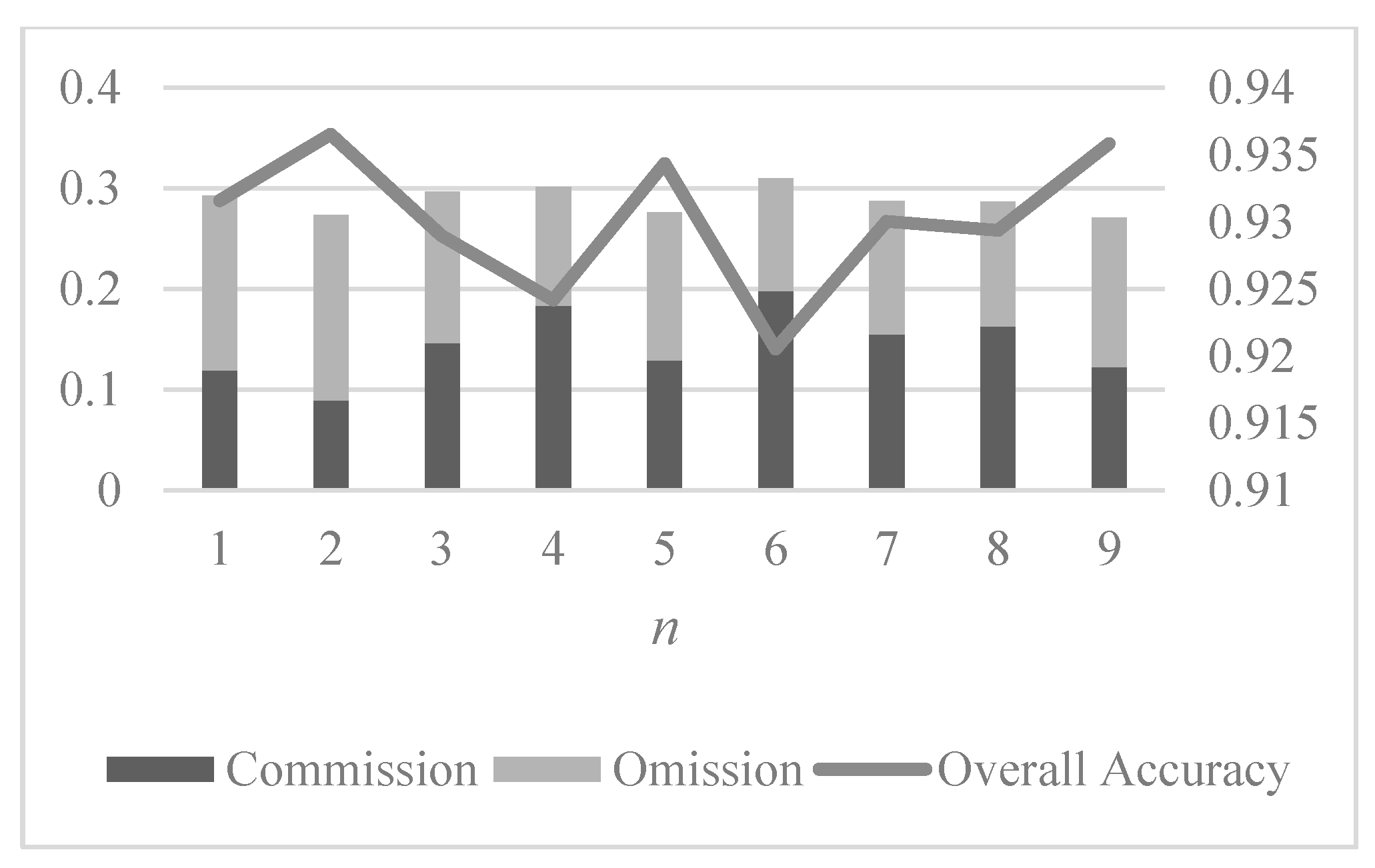
where $x*\prime$ is the location of the target pixel in image #2, and $f\prime (x)$ and $I\prime (x)$, respectively, represent the context prior probability and image intensity in image #2 [30]. After the permanence confidence map is calculated for image #2, obtained after a flood, we select the pixels with top $n\%$ confidence values as the final permanent pixels. In this work, we choose $n=2$. More discussion on how $n$ influences the result will be given later.

3.2. Inundation Mapping Based on Modest AdaBoost

3.2.1. Permanent Pixels Labelling

According to the previous section, we get the set of permanent pixels. In order to utilise the permanent pixels for training the classifier later, we need to label the permanent pixels into water and non-water categories. In keeping the whole process automatic, manual labelling should not be used. In this study, we adopt the openly accessible MODIS 250 m land-water mask, which is called MOD44W for short, to achieve this purpose. MOD44W is a constant product, which is derived from Terra MODIS data MOD44C 250 m 16-day composites. If a pixel is identified as water in more than 50% of the period May to September of years 2000–2002, this pixel is labelled as water in the MOD44W product. This method effectively smooths the short-term water surface changes caused by flood and drought. Therefore, although the MOD44W was produced years before the case study, it is widely accepted as the description of average water distribution [33]. Here, we adopt MOD44W to label the permanent pixels. It is acknowledged that there are most likely some mistakes, caused by small changes in water surface over the years. But, as the general condition changes little, and the permanent pixels have high probability of being unchanged, the labels from MOD44W are generally reliable.

For both the first and second study area, there is only one scene of MOD44W data. We resample the MOD44W data to the same spatial resolution as the experimental image, and then label the permanent pixels into permanent water pixels and permanent non-water pixels according to the MOD44W values. As the labels of the permanent pixels are used for classifier training, the proportion of the permanent pixels of each class will influence the classifier training result. However, as most changes happen inside or around the river regions, it can be inferred that the permanent confidence is generally higher in non-water regions than in water regions. Among the pixels of the highest confidence values, we selected the water and non-water permanent pixels with the same proportion as that in the same scene in MOD44W. The sum of water and non-water permanent pixels remained $n\%$ of the total. With the labelled permanent pixels, the Modest AdaBoost classifier is trained. Then it is applied to the testing set consisting of multiple features of image #2. The final inundation mapping result can be calculated.

3.2.2. Inundation Mapping

Boosting is a technique that combines several weak classifiers to generate a powerful one. The first proposed boosting algorithm, AdaBoost, was created by Freund and Schapire in 1996 [34], which is regarded as the basis for all other kinds of boosting method. Due to its good generalisation ability, low computational complexity and high execution efficiency, boosting has become one of the most popular and effective classification tools in computer vision [35] and pattern recognition [36]. A number of algorithms are derived from the boosting method, such as the Discrete AdaBoost (DADB), Real AdaBoost (RADB) and Gentle AdaBoost (GADB). DADB is a boosting method that mainly employs binary weak classifiers, and RADB is a generalisation version of the basic AdaBoost algorithm [37]. On the basis of RADB, GADB is designed with better performance and higher resistance to outliers [38]. Here, we adopt a different boosting method called Modest AdaBoost, which proves to outperform GADB in generalisation error and overfitting. Its natural stopping criterion is also an advantage, which other boosting techniques lack [36]. The flowchart of mapping inundation using Modest AdaBoost is shown in Figure 4.

Modest AdaBoost is a variant of boosting proposed by A. Vezhnevets et al. [36]. The basic idea of this method is that in every iteration for computing the new distribution, more importance is given to the samples that are misclassified in the previous step (with low margins). In every step, the method is committed to improve the lowest margins of samples. While those training samples that already have high margins may be misclassified with the new distribution and the margins are decreased, this forces the weak classifier to work only in its domain and be ‘modest’, which is the origin of the name MADB. Through this strategy, some regions of the input space have fewer chances to become overconfident, and the generalisation ability of the method benefits from this. The open source GML AdaBoost Matlab Toolbox [39] is used in the experiments to implement the Modest AdaBoost algorithm. It is a collection of classes and functions of several boosting algorithms. More details about the mapping procedure are presented below.

First, each permanent pixel is set as a training sample point. Thus, the training dataset $(x_1,y_1),‥,(x_N,y_N)$ can be obtained. $x_i\in X$ is the input vector, which consists of several feature values of the permanent pixel, and $y_i\in \{-1,+1\}$, which is the corresponding class label of the permanent pixel. Here we define $y=+1$ when the pixel is water, and $y=-1$ when the pixel is non-water. $N$ is the number of permanent pixels. At the beginning, we initialise the weight distribution on the input data as $D_0(i)=1/N$, $i=1,2,\dots ,N$.

For each iteration $t=1,\dots ,T$, with the weight distribution $D_t(i)$, the weak classifier $s_t(x)\in S$ can be trained by weighted least squares:

$$s_t=\underset{s}{{\displaystyle \arg \min }}\left({\displaystyle \sum _{i=1}^N{D}_t(i)\cdot {(y_i-s(x_i))}^2}\right),$$

(12)

In addition, the ‘inverted’ distribution of the data weights is calculated by

$${\overline{D}}_t(i)=(1-D_t(i)){\overline{\alpha }}_t,$$

(13)

where ${\overline{\alpha }}_t$ is the normalisation coefficient. Then we compute the probabilities:

$$P_t^{+1}(x)=P_{D_t}(y=+1\cap s_t(x)),$$

(14)

$${\overline{P}}_t^{+1}(x)=P_{{\overline{D}}_t}(y=+1\cap s_t(x)),$$

(15)

$$P_t^{-1}(x)=P_{D_t}(y=-1\cap s_t(x)),$$

(16)

$${\overline{P}}_t^{-1}(x)=P_{{\overline{D}}_t}(y=-1\cap s_t(x)).$$

(17)

Set

$$f_t(x)=(P_t^{+1}(1-{\overline{P}}_t^{+1})-P_t^{-1}(1-{\overline{P}}_t^{-1}))(x),$$

(18)

and update the distribution by:

$$D_{t+1}(i)=D_t(i)\exp (-y_i{f}_t(x_i)){\alpha }_t,$$

(19)

where ${\alpha }_t$ is the normalisation coefficient. After $T$ iterations or $f_t=0$, the final classifier can be constructed by [36]

$$F(x)=sign[{\displaystyle \sum _{t=1}^T{f}_t(s_t(x))}]$$

(20)

The procedure of training the Modest AdaBoost classifier uses the permanent pixels extracted in previous steps, which contain the typical characteristics of water and non-water. After the strong classifier is obtained, it is applied to image #2 to get the inundation mapping results. Due to the difference in the bands of different satellites, the individual index of fixed band combination cannot always be effective in different flood scenarios. In order to overcome this shortcoming and make the method more robust, we set the components of the training vector using several bands and indices: (1) original bands; (2) $\mathrm{NIR}-\mathrm{Re}\mathrm{d}$; (3) $\mathrm{NIR}/\mathrm{Re}\mathrm{d}$; (4) $\mathrm{EVI}$; (5) $\mathrm{NDVI}$; (6) $\mathrm{NDWI}$. All of these indices can be applied to optical satellite images. The computing method of NDWI is described in (1). For the EVI and the NDVI, the computing methods are as follows [40,41]. The training and classification processes are performed individually on each pixel of the image.

$$\mathrm{EVI}=\frac{2.5\times (\mathrm{NIR}-\mathrm{Red})}{6\times \mathrm{Red}+\mathrm{NIR}-7.5\times \mathrm{Blue}+1},$$

(21)

$$\mathrm{NDVI}=\frac{\mathrm{NIR}-\mathrm{Red}}{\mathrm{NIR}+\mathrm{Red}},$$

(22)

For comparison, the commonly used unsupervised classification method K-MEANs, and another two different permanent pixel extraction methods combined with Modest AdaBoost, are also applied to the same experimental datasets. K-MEANs is implemented using the ENVI 5.0 software. The change threshold is set as 5.0%. One permanent pixel extraction method is from [22], which determines the permanent pixels through the means and mediums of the spatial neighbouring pixels. In another permanent pixel extraction method, a similar judgment rule using mediums and means, but extended to spatiotemporal field, is utilised. Specifically, each pixel has 8 spatial neighbouring pixels, and in the spatial neighbourhood-based permanent pixel extraction method (SP) in [22], if more than 5 among the 8 spatial neighbouring pixels are statistically equal (having the same medium or mean) to the target, the target pixel is considered permanent. For the spatiotemporal neighbourhood-based permanent pixel extraction method (STP), not only more than five spatially neighbouring pixels, but also more than five among the nine temporally neighbouring pixels, need to be statistically equal to the target for the target to be considered permanent. These permanent pixels are utilised with MADB in the same way as the proposed method. The inundation mapping results from each comparison method is then obtained. Here we call these two comparison methods utilising different permanent pixel strategies SP-MADB and STP-MADB, for short. All of these comparison methods are applied on the same multiple feature set of the classification step to the proposed method.

4. Results

4.1. Inundation Mapping Using HJ-1A CCD Data

As described above, in the first case study, two images, acquired on 12 July 2013 (before the flood) and 27 August 2013 (after the flood), are selected for the analysis. After pre-processing, the false colour composite images of the study area and the corresponding MOD44W product used for labelling the training data are shown in Figure 5.

The proposed spatiotemporal-context-learning-based permanent pixels-MADB (STCLP-MADB) method and three other comparison methods (K-MEANs, SP-MADB and STP-MADB) are each respectively applied to the experimental data. The final inundation mapping result for the individual method is shown in Figure 6. For a better visualization of the obtained results, we select four sub-regions and make a detailed zoom in. The location and size of the four sub-regions are shown in Figure 6e. The enlarged view of the small regions and their corresponding false colour composite, flood extraction result and the reference map are shown in Figure 7.

Table 4. The first case study in 2013—Number of inundated pixels.

Method	Full Region	Sub-Region A	Sub-Region B	Sub-Region C	Sub-Region D
K-MEANs	528,238	1833	16,236	7778	1442
SP-MADB	710,587	96	8470	5207	0
STP-MADB	843,570	1750	16,060	7009	1345
STCLP-MADB	812,610	1308	13,884	7011	1047
Reference Map	764,470	1176	11,861	6267	873

lists the number of inundated pixels derived by different methods in the full scene and sub-regions.

From the above figures and table, some comments can be made:

(1)

The proposed inundation mapping method, based on STCL permanent pixel extraction and MADB, successfully extracts most of the flood regions in the first case study. In each column of the Table 4, the STCLP-MADB method achieves the closest number of inundated pixels to the reference, except in sub-region C. It is the second best among the methods, and has almost the same number of inundated pixels as the best. All of this evidence proves the effectiveness of the HJ-1A CCD data and the proposed procedure for mapping wide inundated areas in a river flood event.

(2)

On the whole, it can be seen that the main regions of the flood are mostly well-delineated by each inundation mapping algorithm, except for small tributaries−for example the tributaries near the sub-region A and D−which are omitted by the SP-MADB method, and are shown in yellow. The STCLP-MADB performs better than the three other methods from the visual effect. In these regions, the K-MEANs and STP-MADB results present more false alarms, and the SP-MADB method makes more omissions. The result derived from STCLP-MADB is most consistent with the reference map. Its effectiveness for precision mapping is significant for inferring the future evolution of the flood.

(3)

From the detailed mapping results, it can be found that the inundated regions are delineated differently by different methods. In the map derived using K-MEANs, many points of false positive can be found in the unflooded regions. However, the SP-MADB method produces more false negatives in some small flood regions and half-submerged regions. More advanced results are obtained by STP-MADB and STCLP-MADB methods. Further comparisons of the details show that the results from STCLP-MADB provide finer outlines and are slightly better.

(4)

Although the results from STCLP-MADB are quite promising, there are still some false positive errors, mainly occurring in the small unflooded areas surrounded by large flooded areas. For example, in Figure 6d, we can find some pixels in blue inside the main region of the flood, which are unflooded areas but determined as flood by the STCLP-MADB method. This is because these areas mostly comprise mixed pixels. Different proportions and locations of water in one mixed pixel influence what class the pixel is distributed to.

Besides the qualitative evaluation, a quantitative evaluation is also made for the test. For classification, the confusion matrix is one of the most commonly used methods for calculating accuracy. In this study, the reference and the detection results are all binary maps with two categories, water and non-water. Then, the confusion matrix can be produced. The accuracies of each method can be calculated, among which the overall accuracy is the rate of correctly classified water and non-water pixels among the total pixels. The values are shown in

Table 5. The first case study in 2013—Accuracy.

Method	Overall Accuracy (%)	Kappa	Omission (%)	Commission (%)
K-MEANs	87.48	0.7450	2.77	17.51
SP-MADB	90.73	0.8146	12.18	5.53
STP-MADB	91.22	0.8220	3.03	12.13
STCLP-MADB	92.25	0.8435	4.10	9.78

.

From the numbers reported in Table 5, a few further conclusions can be summarised:

(1)

STCLP-MADB achieves the highest overall accuracy and kappa coefficient among these four methods, which shows that STCLP-MADB performs better than the others in terms of quantitative evaluation. Extending the SP strategy to STP strategy improves mapping accuracy. Furthermore, utilising STCL confidence calculation instead of a simple counting strategy in STP also enhances the mapping results.

(2)

With incomplete flood information, different flood detectors produce different commission and omission errors. The best omission and commission rates are achieved by the K-MEANs and SP-MADB methods, respectively. However, there is always a balance between the omission and the commission. A decrease in omission errors usually brings about an increase in commission errors and vice versa. As can be seen from Table 5, the high commission and omission rates limit the ability of K-MEANs and SP-MADB methods in inundation mapping, which is illustrated in Figure 6 and Figure 7, while the STCLP-MADB method achieves a balance between these two rates and provides a more acceptable result.

We also discuss the relation between accuracy of the proposed method and the $n$ in the permanent pixels extraction step, i.e., the influence that the number of selected permanent pixels has over mapping precision. The result is shown in Figure 8 below. In this work, we try $n=1,2,\dots ,9$, for if $n$ is too big, it will cost a lot of computation resources and time for training the classifier, which is impractical and cannot satisfy the need for a quick response to a disaster.

From the figure, it can be seen that more permanent pixels leads to an increase in commission and decrease in omission, but this only happens when $n\le 2$. When the value of $n$ gets higher, there is no significant change in commission and omission. Similarly, for overall accuracy, there is only a slight decrease (around 0.1%) when $n$ changes from 1 to 2. After that, the overall accuracy remains almost unchanged. Therefore, it can be concluded that for the proposed STCLP-MADB method using HJ-1A CCD data, the number of permanent pixels has a very limited influence on mapping precision. Given the importance of computation efficiency in disaster response, it is quite enough to set $n$ as 1 or 2.

4.2. Inundation Mapping Using GF-4 PMS Data

The second case study aims to analyse the GF-4 PMS data for the 2016 flood event at Dongting Lake. Figure 9 shows the two images selected for this case, which were acquired on 17 June 2016 (before the flood) and 23 July 2016 (after the flood). The corresponding MOD44W product used as the ancillary data is also shown in Figure 9.

In the second case study, inundation mapping results using different strategies are shown in Figure 10. Similar to the first case study, four sub-regions located at different positions are selected and shown in Figure 11, which aims to visually compare the results in a more detailed way. With regards to quantitative evaluation,

Table 6. The second case study in 2016—Number of inundated pixels.

Method	Full Region	Sub-Region A	Sub-Region B	Sub-Region C	Sub-Region D
K-MEANs	2,417,535	74,610	21,785	10,363	13,001
SP-MADB	1,103,408	23,946	1488	5884	6163
STP-MADB	873,738	16,908	1468	5233	3848
STCLP-MADB	1,215,464	30,502	2116	6668	6961
Reference Map	1,357,670	37,529	3654	7963	7510

and

Table 7. The second case study in 2016—Accuracy.

Method	Overall Accuracy (%)	Kappa	Omission (%)	Commission (%)
K-MEANs	79.73	0.5613	3.24	45.66
SP-MADB	92.88	0.7877	26.43	4.29
STP-MADB	91.01	0.7190	36.58	1.46
STCLP-MADB	93.66	0.8195	18.47	8.93

report the number of inundated pixels and the final accuracy values, respectively. Figure 12 illustrates the relation between the permanent pixel proportion and detection accuracy.

As can be seen from the figures and the table, many similarities exist between the results of the second and the first case studies, and several slight differences as well. They are described as follows:

(1)

In terms of the performance in categorisation, results in the second test are similar to that in the first test. The proposed STCLP-MADB method still achieves the best overall accuracy and kappa coefficient. K-MEANs and STP-MADB methods achieve the best omission and commission, respectively, while STCLP-MADB shows an average performance of these two rates. As the two test datasets are from different sensors, locations and inundation cases, this experiment further proves the good robustness of the proposed method.

(2)

K-MEANs makes use of the statistical properties of the whole image, which causes high commission because the inundated pixels can have a different appearance in different contextual situations. SP-MADB and STP-MADB draw more attention to the local characteristics, but they make the determination of permanent pixels by counting, which lacks a theoretical foundation and can be easily disturbed. This can be found by comparing Figure 6c and Figure 10c. In the first case, using HJ-1A CCD data, the STP-MADB method produces more commission, while in the second case study, using GF-4 PMS data, more omission than commission is introduced in the STP-MADB result. In the proposed method, a spatiotemporal context confidence calculating model is adopted to overcome the limitation of counting. With the formulised combination of local spatiotemporal and spectral information, we achieve a more accurate and robust inundation map than other methods.

(3)

The changing curves of accuracy with $n$ are more unstable than those in the first test. The influence of $n$ on result precision does not change monotonically. It is difficult to find any rules in the curves at all. This could be because the outline of the inundation is more complicated in the second case study than in the first. Moreover, the spatial resolution of the GF-4 PMS data is sparser than that of the HJ-1A CCD data, which brings out more mixed pixels. With the increase in these uncertainties, the variation in accuracy becomes more unpredictable. Nevertheless, the fluctuation is still within a limited range. The effectiveness of the proposed method is rather stable.

(4)

As the GF-4 satellite was officially put into service not long ago (in June 2016), research on GF-4 PMS data is rare. Our work explores the applied value of this new dataset and proves its effectiveness for inundation mapping. More promising research about GF-4 PMS data could be carried out in the future.

5. Discussion

In this study, we choose cloud-free images for the experiment. In practice, clouds and their shadows have been a critical issue for flood mapping using multispectral images, especially the as flood is usually accompanied by rainy and cloudy weather. This is because the visible and near infrared spectra cannot penetrate the cloud, so the image quality is frequently affected during flood periods. We put forward some analysis and speculation regarding how this may influence the result of the proposed method. First, the confidence value calculated in the step of STCL will certainly be affected by the clouds. As the STCL method models the correlation of image density and distance, and the cloud has different characteristics with those of the land or the water, the relative relationship will change a lot with the interference of clouds. According to the description in Section 3.1, if there are some clouds present nearby, the confidence value will decrease. However, since we only extract pixels with high confidence values for training the classifier, its impact on the final flood mapping may be limited. On the other hand, the GF-4 is a geostationary satellite. When a disaster happens, it can take images of the same region with a very high time resolution if needed. Through combining the common region of multiple images over a short time, data hidden by clouds and shadows may be recovered. Anyhow, it is a deficiency in our work that no experiment using cloudy data has been carried out. More explorations concerning cloudy data will be made in a future work.

In the proposed process for flood mapping, the MOD44W product plays a role in separating permanent pixels into permanent water pixels and permanent non-water pixels. With the introduction of this water mask, some issues are introduced as well. One is that this product is obtained based on the MODIS data from 2000 to 2002, while our case studies are in 2013 and 2016. There was over a decade between the MOD44W product and the experimental data. The outlines of the water are very likely to have altered. Besides the difference in time, the huge gap between the spatial resolutions of the water mask and the experimental data could also lead to problems. The spatial resolution of the MOD44W product is 250 m, which is much lower than that of the HJ-1A/B CCD and GF-4 PMS data. Many jagged edges can be found in the resampled result of the MOD44W product. Moreover, some small water surfaces are omitted because of the low spatial resolution. Both of these issues will bring about errors in labelling the permanent pixels. Nevertheless, as the labelled permanent pixels serve as the training set for the Modest AdaBoost classifier, not the final detailed classification result, we think a certain number of errors can be tolerated. Figure 5c and Figure 9c also show that, in the experimental areas, from the visual effect, the MOD44W product is able to provide a general outline of the water before the flood comes. From another perspective, for the areas near the edges of the rivers and lakes, where most of the differences between the MOD44W product and the study data exist, the confidence value is generally low because of the changes induced by the flood. Therefore, the pixels at these areas are less likely to be selected as permanent pixels, and their corresponding MOD44W labels would have little influence on the final result.

According to the demand for automation and details in disaster assessment, this study aims to explore a novel solution for flood mapping that can achieve precise results with minimal human intervention. After two experiments on different regions and data, the proposed method shows better performance than other automatic methods. Several important reasons we infer are as follows. The first is the introduction of the machine learning classification method. Extensive literature shows that the precision of supervised classification methods is generally better than that of unsupervised classification methods. Unsupervised flood mapping methods, like K-MEANs, can bring about more errors in scenes of large area or complicated distribution. Because in these situations, the radiation value of water may vary a lot at different locations. Without a learning strategy, some non-water pixels with similar features to the water at other locations could be identified as water, as can be seen in Figure 10a of the Dongting Lake case. With the aid of the samples, the supervised classifier can learn and adapt itself better to different land cover characteristics in different scenes, resulting in higher accuracy. But the samples usually need to be selected manually, which limits their applicability in disaster response. Another essential advantage of the proposed method is that it proposes an automatic sample selection method, and combines it with a learning method. With the advantages of these two methods, both good precision and automation can be achieved.

The utilisation of local information is also a factor bringing improvement to the result. On one hand, it is more robust to utilise both contextual and global information than to utilise global information only. On the other hand, the experiment results show that the proposed method outperforms (qualitatively and quantitatively) the SP-MADB, STP-MADB methods. The only distinction among these three methods is the permanent pixel extraction strategy. All three methods utilise the local relationship between a pixel and its surroundings. The SP-MADB and STP-MADB methods count the number of 8-neighbourhood or 17-neighbourhood pixels with equal mean or medium to the object pixel. Noise and radiation variation, which exist all the time, can easily change the count result. Moreover, if a pixel and its neighbouring pixels simultaneously change from one cover type to another, the mean and medium will still remain the same, leading to errors in the permanent pixel set. From the experiment results we can see that the STP-MADB method obviously makes more commissions than omissions in the first case study, but makes more omissions in the second case, which proves its lack of robustness. Whereas, the proposed method builds a model between the pixel and its neighbouring regions, instead of counting the few adjacent pixels. Even if there are some noise pixels, the general structure of the model will not change. With better selection of the permanent pixels and the training set, the STCLP-MADB method produces a more precise outline of the inundated areas.

This study is proposed for floods, which is a practical problem. Hence it makes sense that this proposed method can be applied operationally, and that it can help when a real flood comes. Here we propose some suggestions for implementation, which may help the STCL-MADB method to be effectively applied in a real application. The whole workflow can be divided into three steps: extracting permanent pixels using STCL, training the classifier and mapping the inundation. The first step, especially the STCL algorithm, accounts for most of the time consumption in the whole process. Not only because the STCL algorithm has higher computation complexity than other steps, but the operations need to be performed pixel by pixel. For example, in the second case study at Dongting Lake, the size of the data is 2534 × 2235 pixels. The first step takes around 3 days, while the second and third steps take around 15 min and a few dozen seconds, respectively. All these experiments are implemented by MATLAB 2013 on a laptop with an i7-4710HQ CPU and 8 GB RAM. In practice, a library of permanent pixels can be built in advance for regions with high flood risk. With the accumulation of time series data, the library can be updated continuously. Then, the classifier can also be trained and updated with the new library. As soon as the latest scene of remote sensing data arrives, the ready classifier can be directly applied to it. In addition, implementing the process in other programming languages and utilising high-performance processors could also help promote efficiency. Above all, remote sensing data with middle-high spatial and temporal resolution are recommended in the proposed method, as the spatiotemporal contextual information in the image is important for the method. If the spatial or the temporal resolution is rather low in the data, the correlation between neighbouring pixels could be unremarkable.

6. Conclusions

Due to its vast coverage in spatial and temporal scales, flood is considered to be one of the most complex disasters in the world. A novel inundation mapping approach based on spatiotemporal context learning and Modest AdaBoost is proposed and verified in this paper. The proposed method is implemented and evaluated in two different flooding cases using images from different sensors, HJ-1A CCD and GF-4 PMS. The experimental results show that the proposed approach is effective, and is able to produce more accurate mapping results than other state-of-the-art methods and, more importantly, without any artificial samples and thresholds.

On one hand, compared with the traditional global-based unsupervised flood mapping methods (such as K-MEANs), the SP-MADB, STP-MADB and the proposed method combine an automatic sample selection strategy with a machine learning classifier, leading to higher accuracies in an automatic way. With the samples extracted using local information, each of these three methods achieves an overall accuracy of more than 90% in both of the first and second case studies. By comparing the results of the SP-MADB and STP-MADB methods, it can be seen that only extending the neighbouring region to the temporal domain cannot significantly improve the performance of the SP-MADB method. With a formulised model of the spatiotemporal context information instead of simple counting, the proposed approach achieves a more accurate and robust result than other methods. As a result of mixed pixels, there are still some inaccuracies in the result. Moreover, the effect of the proposed method on cloudy data needs to be explored. Future work will focus on these aspects and validate the proposed method with more kinds of data.

References

1. O’Keefe, P.; Westgate, K.; Wisner, B. Taking the naturalness out of natural disasters. Nature 1976, 260, 566–567. [Google Scholar] [CrossRef]
2. Sanyal, J.; Lu, X.X. Application of remote sensing in flood management with special reference to monsoon Asia: A review. Nat. Hazards 2004, 33, 283–301. [Google Scholar] [CrossRef]
3. Berz, G.; Kron, W.; Loster, T.; Rauch, E.; Schimetschek, J.; Schmieder, J.; Siebert, A.; Smolka, A.; Wirtz, A. World map of natural hazards—A global view of the distribution and intensity of significant exposures. Nat. Hazards 2001, 23, 443–465. [Google Scholar] [CrossRef]
4. Akıncı, H.; Erdoğan, S. Designing a flood forecasting and inundation-mapping system integrated with spatial data infrastructures for Turkey. Nat. Hazards 2014, 71, 895–911. [Google Scholar] [CrossRef]
5. Smith, L.C. Satellite remote sensing of river inundation area, stage, and discharge: A review. Hydrol. Process. 1997, 11, 1427–1439. [Google Scholar] [CrossRef]
6. Brivio, P.A.; Colombo, R.; Maggi, M.; Tomasoni, R. Integration of remote sensing data and GIS for accurate mapping of flooded areas. Int. J. Remote Sens. 2002, 23, 429–441. [Google Scholar] [CrossRef]
7. Wang, Y.; Colby, J.D.; Mulcahy, K.A. An efficient method for mapping flood extent in a coastal floodplain using Landsat TM and DEM data. Int. J. Remote Sens. 2002, 23, 3681–3696. [Google Scholar] [CrossRef]
8. Rahman, M.S.; Di, L. The state of the art of spaceborne remote sensing in flood management. Nat. Hazards 2017, 85, 1223–1248. [Google Scholar] [CrossRef]
9. Li, L.; Chen, Y.; Yu, X.; Liu, R.; Huang, C. Sub-pixel flood inundation mapping from multispectral remotely sensed images based on discrete particle swarm optimization. ISPRS J. Photogramm. Remote Sens. 2015, 101, 10–21. [Google Scholar] [CrossRef]
10. Brakenridge, R.; Anderson, E. MODIS-based flood detection, mapping and measurement: The potential for operational hydrological applications. In Transboundary Floods: Reducing Risks through Flood Management; Marsalek, J., Stancalie, G., Balint, G., Eds.; Springer: Dordrecht, The Netherlands, 2006; Volume 72, pp. 1–12. [Google Scholar]
11. Ticehurst, C.J.; Chen, Y.; Karim, F.; Dutta, D.; Gouweleeuw, B. Using MODIS for mapping flood events for use in hydrological and hydrodynamic models: Experiences so far. In Proceedings of the 20th International Congress on Modelling and Simulation, Adelaide, Australia, 1–6 December 2013; pp. 1–6. [Google Scholar]
12. Kwak, Y.; Park, J.; Yorozuya, A.; Fukami, K. Estimation of flood volume in Chao Phraya River basin, Thailand, from MODIS images couppled with flood inundation level. In Proceedings of the 2012 IEEE International Geoscience and Remote Sensing Symposium (IGARSS), Munich, Germany, 22–27 July 2012. [Google Scholar]
13. Khan, S.I.; Hong, Y.; Wang, J.; Yilmaz, K.K.; Gourley, J.J.; Adler, R.F.; Brakenridge, G.R.; Policelli, F.; Habib, S.; Irwin, D. Satellite remote sensing and hydrologic modeling for flood inundation mapping in Lake Victoria basin: Implications for hydrologic prediction in ungauged basins. IEEE Trans. Geosci. Remote Sens. 2011, 49, 85–95. [Google Scholar] [CrossRef]
14. Schumann, G. Preface: Remote Sensing in Flood Monitoring and Management. Remote Sens. 2015, 7, 17013–17015. [Google Scholar] [CrossRef]
15. McFeeters, S.K. The use of the Normalized Difference Water Index (NDWI) in the delineation of open water features. Int. J. Remote Sens. 1996, 17, 1425–1432. [Google Scholar] [CrossRef]
16. Jain, S.K.; Singh, R.D.; Jain, M.K.; Lohani, A.K. Delineation of flood-prone areas using remote sensing techniques. Water Resour. Manag. 2005, 19, 333–347. [Google Scholar] [CrossRef]
17. Xie, H.; Luo, X.; Xu, X.; Pan, H.; Tong, X. Evaluation of Landsat 8 OLI imagery for unsupervised inland water extraction. Int. J. Remote Sens. 2016, 37, 1826–1844. [Google Scholar] [CrossRef]
18. Giordano, F.; Goccia, M.; Dellepiane, S. Segmentation of coherence maps for flood damage assessment. In Proceedings of the IEEE International Conference on Image Processing, Genova, Italy, 14 September 2005; Volume 2, p. II-233. [Google Scholar]
19. Dellepiane, S.; Angiati, E.; Vernazza, G. Processing and segmentation of COSMO-SkyMed images for flood monitoring. In Proceedings of the 2010 IEEE International Geoscience and Remote Sensing Symposium, Honolulu, HI, USA, 25–30 July 2010. [Google Scholar]
20. Chignell, S.M.; Anderson, R.S.; Evangelista, P.H.; Laituri, M.J.; Merritt, D.M. Multi-temporal independent component analysis and Landsat 8 for delineating maximum extent of the 2013 Colorado front range flood. Remote Sens. 2015, 7, 9822–9843. [Google Scholar] [CrossRef]
21. Rokni, K.; Ahmad, A.; Selamat, A.; Hazini, S. Water feature extraction and change detection using multitemporal Landsat imagery. Remote Sens. 2014, 6, 4173–4189. [Google Scholar] [CrossRef]
22. Chen, X.C.; Khandelwal, A.; Shi, S.; Faghmous, J.H.; Boriah, S.; Kumar, V. Unsupervised method for water surface extent monitoring using remote sensing data. In Machine Learning and Data Mining Approaches to Climate Science; Springer International Publishing: Cham, Switzerland, 2015; pp. 51–58. [Google Scholar]
23. Huang, C.; Chen, Y.; Wu, J. Dem-based modification of pixel-swapping algorithm for enhancing floodplain inundation mapping. Int. J. Remote Sens. 2014, 35, 365–381. [Google Scholar] [CrossRef]
24. Lu, S.; Wu, B.; Yan, N.; Wang, H. Water body mapping method with hj-1a/b satellite imagery. Int. J. Appl. Earth Obs. Geoinf. 2011, 13, 428–434. [Google Scholar] [CrossRef]
25. Gu, X.; Tong, X. Overview of china earth observation satellite programs. IEEE Geosci. Remote Sens. Mag. 2015, 3, 113–129. [Google Scholar]
26. Gu, Y.; Hunt, E.; Wardlow, B.; Basara, J.B.; Brown, J.F.; Verdin, J.P. Evaluation of MODIS NDVI and NDWI for vegetation drought monitoring using oklahoma mesonet soil moisture data. Geophys. Res. Lett. 2008, 35, 1092–1104. [Google Scholar] [CrossRef]
27. George, C.; Rowland, C.; Gerard, F.; Balzter, H. Retrospective mapping of burnt areas in central siberia using a modification of the normalised difference water index. Remote Sens. Environ. 2006, 104, 346–359. [Google Scholar] [CrossRef]
28. Mcfeeters, S.K. Using the normalized difference water index (NDWI) within a geographic information system to detect swimming pools for mosquito abatement: A practical approach. Remote Sens. 2013, 5, 3544–3561. [Google Scholar] [CrossRef]
29. Li, W.; Du, Z.; Ling, F.; Zhou, D.; Wang, H.; Gui, Y.; Sun, B.; Zhang, X. A comparison of land surface water mapping using the normalized difference water index from TM, ETM+ and ALI. Remote Sens. 2013, 5, 5530–5549. [Google Scholar] [CrossRef]
30. Zhang, K.; Zhang, L.; Yang, M.H.; Zhang, D. Fast tracking via spatio-temporal context learning. arXiv, 2013; preprint. arXiv:1311.1939. [Google Scholar]
31. Zuo, Z.Y.; Tian, S.; Pei, W.Y.; Yin, X.C. Multi-strategy tracking based text detection in scene videos. In Proceedings of the IEEE 13th International Conference on Document Analysis and Recognition, Tunis, Tunisia, 23–26 August 2015. [Google Scholar]
32. Xu, J.; Lu, Y.; Liu, J. Robust tracking via weighted spatio-temporal context learning. In Proceedings of the 2014 IEEE International Conference on Image Processing (ICIP), Paris, France, 27–30 October 2014. [Google Scholar]
33. Muster, S.; Heim, B.; Abnizova, A.; Boike, J. Water body distributions across scales: A remote sensing based comparison of three arctic tundra wetlands. Remote Sens. 2013, 5, 1498–1523. [Google Scholar] [CrossRef]
34. Freund, Y.; Schapire, R.E. A desicion-theoretic generalization of on-line learning and an application to boosting. In European Conference on Computational Learning Theory; Springer: Berlin/Heidelberg, Germany, 1995; pp. 23–37. [Google Scholar]
35. Viola, P.; Jones, M. Robust real-time object detection. Int. J. Comput. Vis. 2001, 57, 34–37. [Google Scholar]
36. Vezhnevets, A.; Vezhnevets, V. Modest AdaBoost-teaching AdaBoost to generalize better. Graphicon 2005, 12, 987–997. [Google Scholar]
37. Sam, K.T.; Tian, X.L. Rapid license plate detection using Modest AdaBoost and template matching. In Proceedings of the 2nd International Conference on Digital Image Processing, Singapore, 26 February 2010. [Google Scholar]
38. Qahwaji, R.; Al-Omari, M.; Colak, T.; Ipson, S. Using the real, gentle and modest AdaBoost learning algorithms to investigate the computerised associations between coronal mass ejections and filaments. In Proceedings of the 2008 IEEE Communications, Computers and Applications, Amman, Jordan, 8–10 August 2008. [Google Scholar]
39. MSU Graphics & Media Lab, Computer Vision Group. Available online: http://graphics.cs.msu.ru (accessed on 3 June 2016).
40. Gao, B.C. NDWI—A normalized difference water index for remote sensing of vegetation liquid water from space. Remote Sens. Environ. 1996, 58, 257–266. [Google Scholar] [CrossRef]
41. Huete, A.; Didan, K.; Miura, T.; Rodriguez, E.P.; Gao, X.; Ferreira, L.G. Overview of the radiometric and biophysical performance of the MODIS vegetation indices. Remote Sens. Environ. 2002, 83, 195–213. [Google Scholar] [CrossRef]
Figure 1. (a) Location of the first study site near the border of Russia and China; (b) Extent of the HJ-1A CCD data used in this study.
Remotesensing 09 00617 g001
Figure 2. (a) Location of the second study site at the North of Hunan Province in China; (b) Extent of the GF-4 PMS data used in this study.
Remotesensing 09 00617 g002
Figure 3. Flowchart of permanent pixel extraction procedure.
Remotesensing 09 00617 g003
Figure 4. Flowchart of inundation mapping procedure.
Remotesensing 09 00617 g004
Figure 5. False colour composites (R4G3B2) of HJ-1A CCD images acquired on (a) 12 July 2013 (before the flood) and (b) 27 August 2013 (after the flood) for the first case study. (c) Corresponding MOD44W water mask product with water in blue and land in black.
Remotesensing 09 00617 g005
Figure 6. (ad) Flood inundation mapping results for the first case study using K-MEANs, SP-MADB, STP-MADB and STCLP-MADB methods. (Gray: flood pixels in both the detection and reference maps; Blue: flood pixels only in the detection map; Yellow: flood pixels only in the reference map; Black: the background). (e) The locations of the four sub-regions in red rectangle, shown on the reference map of inundation derived from the GF-1 WFV data, with the water in yellow and the background in black.
Remotesensing 09 00617 g006
Figure 7. From the left to the right column: the regions of interest A, B, C and D for the first case study. From the second to the fifth row: corresponding detection and reference maps with the flood in blue and the background in black.
Remotesensing 09 00617 g007
Figure 8. The first case study: commission, omission and overall accuracy in function of n , the percentage of permanent pixels.
Remotesensing 09 00617 g008
Figure 9. False colour composites (R: 5, G: 4, B: 3) of GF-4 PMS images acquired on (a) 17 June 2016 (before the flood) and (b) 23 July 2016 (after the flood) for the second test case. (c) Corresponding MOD44W water mask product with water in blue and land in black.
Remotesensing 09 00617 g009
Figure 10. (ad) Flood inundation mapping results for the second test area using K-MEANs, SP-MADB, STP-MADB and STCLP-MADB methods. (Gray: flood pixels in both the detection and reference maps; Blue: flood pixels only in the detection map; Yellow: flood pixels only in the reference map; Black: the background). (e) The locations of the four sub-regions in red rectangle, shown on the reference map of inundation derived from the HJ-1B CCD data, with the water in yellow and the background in black.
Remotesensing 09 00617 g010
Figure 11. From the left to the right column: the regions of interest A, B, C and D for the second case study. From the second to the fifth row: corresponding detection and reference maps with the flood in blue and the background in black.
Remotesensing 09 00617 g011
Figure 12. Second test—commission, omission and overall accuracy in function of n , the percentage of permanent pixels.
Remotesensing 09 00617 g012