
Improved Model for Depth Bias Correction in Airborne LiDAR Bathymetry Systems


1
School of Geodesy and Geomatics, Wuhan University, 129 Luoyu Road, Wuhan 430079, China
2
Institute of Marine Science and Technology, Wuhan University, Wuhan 430079, China
3
Automation Department, School of Power and Mechanical Engineering, Wuhan University, Wuhan 430072, China
4
The Survey Bureau of Hydrology and Water Resources of Yangtze Estuary, Shanghai 200136, China
*
Author to whom correspondence should be addressed.
Remote Sens. 2017, 9(7), 710; https://0-doi-org.brum.beds.ac.uk/10.3390/rs9070710
Submission received: 24 May 2017
/
Revised: 5 July 2017
/
Accepted: 6 July 2017
/
Published: 10 July 2017
(This article belongs to the Section Ocean Remote Sensing)
Abstract
:Airborne LiDAR bathymetry (ALB) is efficient and cost effective in obtaining shallow water topography, but often produces a low-accuracy sounding solution due to the effects of ALB measurements and ocean hydrological parameters. In bathymetry estimates, peak shifting of the green bottom return caused by pulse stretching induces depth bias, which is the largest error source in ALB depth measurements. The traditional depth bias model is often applied to reduce the depth bias, but it is insufficient when used with various ALB system parameters and ocean environments. Therefore, an accurate model that considers all of the influencing factors must be established. In this study, an improved depth bias model is developed through stepwise regression in consideration of the water depth, laser beam scanning angle, sensor height, and suspended sediment concentration. The proposed improved model and a traditional one are used in an experiment. The results show that the systematic deviation of depth bias corrected by the traditional and improved models is reduced significantly. Standard deviations of 0.086 and 0.055 m are obtained with the traditional and improved models, respectively. The accuracy of the ALB-derived depth corrected by the improved model is better than that corrected by the traditional model.
1. Introduction
Airborne LiDAR bathymetry (ALB) is an accurate, cost-effective, and rapid technique for shallow water measurements [1,2,3,4,5,6]. Aside from its use in traditional nautical charting, ALB is also widely utilized to monitor engineering structures, sand movement, and environmental changes, as well as in resource management and exploitation [7,8,9,10]. ALB can also be used to produce environmental products, such as seafloor reflectance images, seafloor classification maps, and water column characterization maps [11].
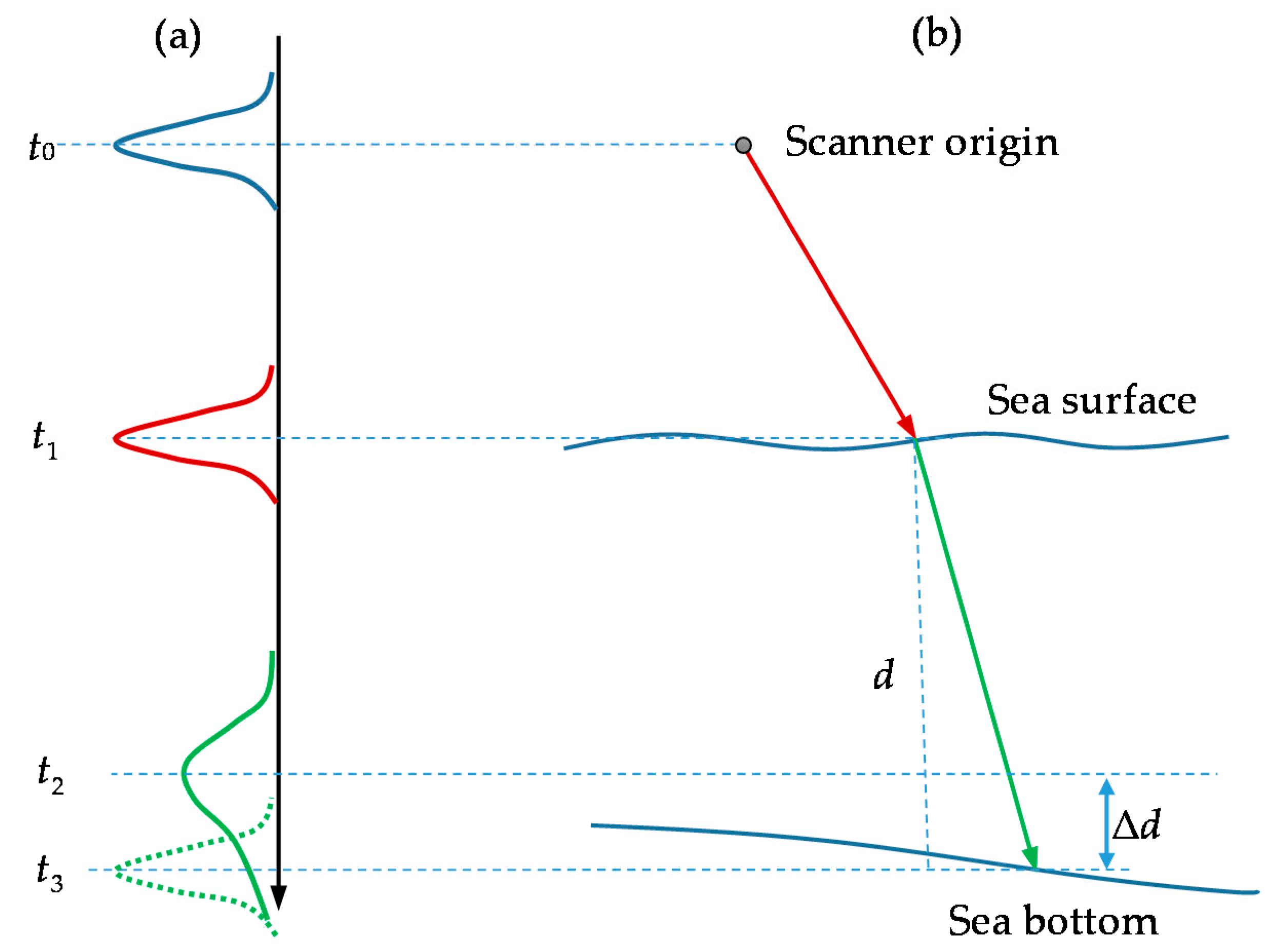
Figure 1 shows the principle of ALB measurements. Bathymetric accuracy is an essential requirement for a successful ALB system, and it is primarily affected by ALB measurement and ocean hydrological parameters. ALB bathymetric errors can be resolved by two components: depth bias and residuals [12]. For an integrated infrared (IR) and green ALB system in which an additional IR laser is used to detect the water surface accurately, depth bias is mainly induced by pulse stretching of the green bottom return [2,13,14]. Geometric dispersion and multiple scattering lead to temporal stretching of the received green bottom return, and this phenomenon is known as the pulse stretching effect [1,2,3,13,14,15,16]. The pulse waveform is distorted (e.g., peak shifting) by the pulse stretching effect. Peak shifting induces bias in bathymetry estimates that is based on a peak detection of up to 92% of the true water depth [14]. This depth bias is the largest source of error in ALB depth measurements. Water surface waves also affect depth bias. As energy is put into the water surface by wind, small capillary waves develop [17]. As the water gains energy, the waves increase in height and length. When they exceed 0.0174 m in length, they take on the shape of the sine curve and become gravity waves [17]. Increased energy increases the steepness of the waves [17]. Different surface slope values may steer laser rays away from the original ray path, resulting in angle and depth biases. Depth bias can be corrected through theoretical analysis [2,14], empirical modeling [12,18,19], and the error statistics method [20,21].
The Monte Carlo numerical method and the analytical approach are two classic theoretical analysis methods [15]. A Monte Carlo simulation is used to estimate depth biases with the impulse response function (IRF), which is a function of the beam scanning angle, sea depth, phase function, optical depth, and single-scattering albedo [2]. Single-scattering albedo is a main parameter in IRF and can be obtained by estimating the scattering coefficient. However, estimating scattering coefficients accurately and efficiently is difficult. Depth biases induced by peak shifting can be analyzed with the Water LiDAR (Wa-LID) simulator [14]. Wa-LID was developed to simulate the reflection of LiDAR waveforms from water across visible wavelengths [22]. The relationship among the time shifts of waveform peaks, bottom slope, water depth, and footprint size is modeled with the Wa-LID simulator [14]. However, the model is based on the assumptions of a vertical incident beam and homogeneous water clarity, which are inconsistent with actual circumstances.
By combining bathymetric ALB and sonar data, an empirical model to depict ALB depth bias was established in a previous study through regression analysis; the model is a function of water depth only [12,18]. The ALB depth corrected by this model can meet the requirements of only several low-accuracy applications because the two parameters cannot fully reflect ALB depth bias. Wright et al. [19] improved the depth bias model by adding a constant term. This model is also a function of water depth only and is simple to establish, but its adaptability to complex and variable ALB measurement and ocean hydrological parameters is weak. Therefore, an accurate model that considers all influencing factors must be built.
The error statistics method is often used to correct ALB depth biases in river measurements [20,21]. The magnitude and spatial variation of depth bias can be evaluated by referring to ground surveying results and can be obtained by subtracting ground surveying elevations from ALB-derived elevations. The error statistics shows that depth bias has low relevance with local topographic variance or flow depth and can be corrected by subtracting the mean bias from raw ALB-derived depths. This method is simple and efficient in correcting depth biases in water areas with small depth variations and has been applied successfully in rivers by Hilldale et al. [20] and Skinner et al. [21]. However, the method is difficult to apply in water areas with complicated depth variations.
All of these methods improve the ALB bathymetric accuracy to a certain extent. The error statistics method is simple and highly efficient, but its adaptability to complex ocean hydrological environments is weak. The theoretical analysis method provides an understanding of the physical processes involved, but it is limited by simplified assumptions that may be inconsistent with the actual ocean hydrological environment; therefore, it requires further improvement. The empirical modeling method can be used to establish a model of the relationship between ALB depth bias and influencing factors in a specific environment. This method is simple and easy to implement. However, in the empirical model, the parameters that influence depth bias should be completely identified, and their significance should be fully analyzed. Otherwise, the established empirical model may result in low-accuracy correction.
An improved model for ALB depth bias correction is developed in this study by analyzing ALB bathymetric mechanisms and the factors that influence ALB depth accuracy. The proposed model considers various parameters, such as the water depth, turbidity, beam scanning angle, and sensor height.
This paper is structured as follows. Section 2 provides the detailed method of building the proposed depth bias model. Section 3 presents the validation and analysis of the proposed method through experiments. Section 4 provides the corresponding discussions. Section 5 presents the conclusions and recommendations obtained from the experiments and discussions.
2. Building the Depth Bias Model
2.1. Influencing Factors and Depth Bias Model
With the sonar-derived water depth as a reference, ALB depth bias can be obtained by comparing the ALB-derived depth with the reference. Penny et al. [12] and Brain et al. [18] analyzed the error distribution, found that ALB depth bias ∆d varies with water depth d, and built a simple linear bias model Equation (1) to depict the bias.
where β is the model coefficient. Wright et al. [19] improved Brain’s depth bias model by adding a constant term, b, as follows:
Model coefficient β indicates the rate by which depth bias changes with water depth. Aside from water depth d, ∆d should also be related to the hydrological parameters of seawater (i.e., water turbidity) and measurement parameters of ALB systems (i.e., beam scanning angle and laser footprint size) [1,2,3,14,15,16]. Therefore, the traditional linear model depicted in Equation (2) needs to be extended as:
where b is a constant term, β is the depth bias coefficient, Turb is the water turbidity, φ is the beam scanning angle, F is the LiDAR footprint size, and α1–α7 are the model coefficients.
The correlations between turbidity and suspended sediment concentration (SSC) have been investigated through extensive experiments [23,24,25,26,27,28,29]. Although turbidity depends on SSC, as well as particle composition and size distribution, many experiments have shown that a good linear relationship exists between turbidity and SSC [23,25,27,28,29]. Therefore, Turb is expressed as follows:
where C is SSC, and k and m are coefficients that vary in different regions and times. However, these coefficients can be regarded as constants in the same region and in a short period [23,25,27,28,29].
F can be calculated with the sensor height H and LiDAR divergence angle γ [14] using the following equation:
An ALB system determines the transmitted pulse characteristics (i.e., initial radius and divergence) [30]. Thus, γ should no longer be included in the depth bias model as an independent variable. The following equation was obtained when Equations (4) and (5) were substituted into Equation (3):
where β is the model coefficient, which is a function of the beam scanning angle φ, sensor height H, and SSC C. Equation (6) is the initial depth bias model proposed in this study and should be further optimized. Equation (6) does not consider the effect of the water surface and regards the water surface as flat. The wave effect will be discussed in Section 4.
2.2. Development of the Depth Bias Model
The initial model depicted in Equation (6) can be built by using the following data:
- (1)
- Seabed elevations derived from ALB and sonar at the same locations.
- (2)
- Ocean hydrological parameters of the ALB survey water (i.e., SSC C) and ALB measurement parameters (i.e., beam scanning angle φ and sensor height H).
ALB depth bias ∆d can be calculated with the water depths derived from ALB and sonar at the same location, as follows:
where DALB is the ALB-derived water depth after chart datum correction and Dsonar is the sonar-derived water depth after chart datum correction.
For the seabed topography produced from ALB and sonar, the following equation can be derived:
where Hdatum is the ellipsoid height of the chart datum and HBALB and HBSonar are the seabed ellipsoid heights derived by ALB and sonar, respectively. Therefore, ∆d can be obtained by comparing HBALB and HBSonar at the same location, as follows:
For ALB measurements on the spot, Equation (9) can be transformed into:
where HSALB and dALB are the sea surface ellipsoid heights derived by the ALB IR channel and the ALB-derived depth at the time of the ALB measurement, respectively. Tsonar and dsonar are the tidal level defined on the ellipsoid surface and the sounding result at the time of the sonar sounding, respectively. dALB can be calculated by subtracting HSALB from HBALB, as follows:
HBALB, φ, and H can be extracted from raw ALB records. HBSonar can be extracted from sonar records. C can be obtained through on-site sampling and a laboratory analysis. After obtaining these data, the improved depth bias model presented in Equation (6) can be established. The matrix form can be expressed as:
where m is the number of point pairs in the ALB and sonar surveying points at the same locations.
X can be calculated based on the least squares principle as follows:
2.3. Variable Selection for the Depth Bias Model
Theory and experience give only a general direction as to which of a pool of candidate variables (including transformed variables) should be included in the initial depth bias model. The actual set of predictor variables used in the final regression model must be determined by analysis of the data. Determining this subset is called the variable selection problem. The goal of variable selection is conflicting: achieving a balance between simplicity (i.e., as few regressors as possible) and fit (i.e., as many regressors as needed) [31]. Variable selection for the depth bias model can be implemented through stepwise regression.
The depth bias model shown in Equation (6) is only an initial model that considers the main influencing factors and can be optimized through stepwise regression. A t-test was adopted to conduct significance tests on the regression coefficients of the depth bias model. Detailed descriptions of the stepwise regression and t-test theories are provided in Appendix A.
3. Experiment and Analysis
3.1. Data Acquisition
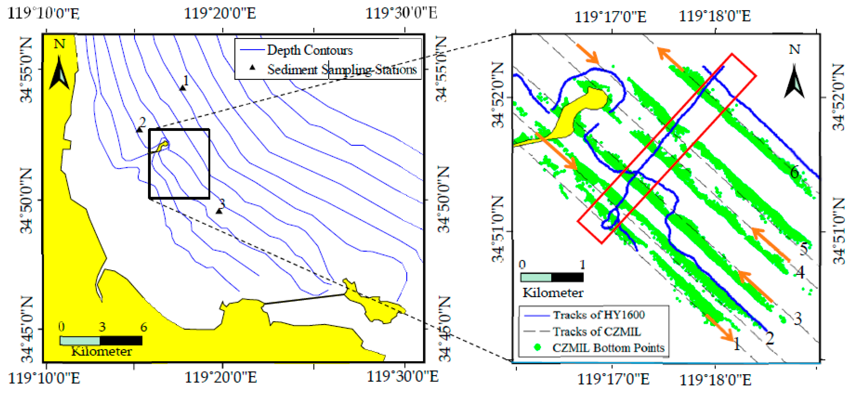
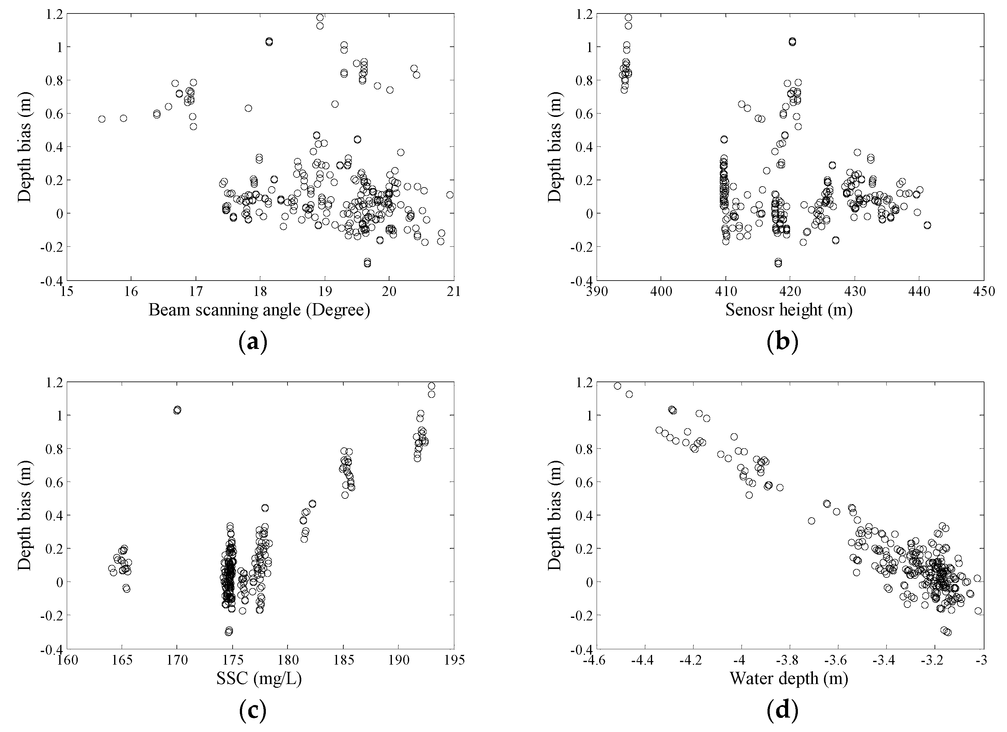
A comprehensive survey was conducted in a high-turbidity water area (5 km × 5 km) near Lianyungang, Jiangsu Province, China, to evaluate the reliability and accuracy of the proposed method. Six-line ALB data were collected with Coastal Zone Mapping and Imaging LiDAR (CZMIL). The primary technical parameters of CZMIL are listed in Table 1. Six flight lines were planned before the ALB measurement. Three flights (lines 1, 2, and 5) were carried out from northwest to southeast, and three other flights (lines 3, 4, and 6) were carried out along the opposite direction. Sonar sounding and suspended sediment sampling were conducted in the same water area. HY1600, an echo sounding system that has an accuracy of ±(0.01 m + 0.001 d), was adopted. The sounding tracks are displayed in Figure 2. Meanwhile, three suspended sediment sampling stations were arranged around the survey area, as shown in Figure 2. Seawater samples were collected by using horizontal water samplers in situ and analyzed in the laboratory. Suspended sediment sampling was performed only in the surface, middle, and bottom layers at each sampling station because of the shallow depth, and the mean of the different layer results was used as the SSC for each sampling station. The locations and scopes of the different measurements are shown in Figure 2. The SSCs of the three sampling stations are listed in Table 2.
3.2. Model Construction
Raw ALB data were processed with Optech HydroFusion software, and the seabed elevation of each ALB surveying point was obtained. The seabed elevations were obtained by processing HY1600 data with the Hypack software. The nearest ALB point around a sonar point within a 1.0 m radius can be used to form a point pair with the sonar point because the seabed topography changes gradually. With the sonar sounding result as a reference, the ALB depth biases of each point pair, ∆d, can be calculated with Equation (9).
Figure 3d shows that ∆d varies approximately linearly with the water depth. A constant bias or an interception exists between them, which indicates that the linear depth bias model in Equation (6) is appropriate. In addition, the sensor height H and beam scanning angle φ in each measuring point were extracted from raw ALB records. The SSC in each measuring point was determined through inverse distance weighting (IDW) interpolation using SSC and the coordinates of the SSC sampling stations (Table 2). IDW is extensively used to interpolate spatial data (e.g., SSC) and is considered an effective method [32,33,34]. A detailed description of IDW theory is provided in Appendix A. The interpolation in this study adopted the assumption that the change in SSC among the sampling stations is gradual.
When the ALB sounding point was approximately in the same location as the sonar sounding point, the two sounding points from CZMIL and HY1600 were defined as a point pair. A total of 379 point pairs were found in the surveyed water area. A total of 317 point pairs were selected randomly to construct the depth bias model, and the remaining 62 point pairs were used to assess the model. The measurement and ocean hydrological parameters used in model construction are shown in Table 3 and Figure 3. Evidently, Δd ranges from −0.16 m to 1.22 m and has a mean of 0.16 m and standard deviation of 0.29 m. This result implies that raw ALB-derived depth bias is significant. Thus, a depth bias model should be built to improve the accuracy of the ALB-derived depth.
With these data, the initial depth bias model depicted in Equation (6) was constructed. A t-test was performed to conduct hypothesis tests on the regression coefficients and evaluate the significance of the model parameters. The test results are shown in Table 4. The standard error (SE), t-statistics (t), and p-value (p) of each coefficient were calculated and the results are shown in Table 4. A comparison of the p-values of these coefficients showed that all coefficients, except for β6, β7, and b, were higher than the standard α = 0.05 cutoff, indicating that multicollinearity exists in the initial model shown in Equation (6) and that the model cannot substantially represent depth bias. To solve this problem, stepwise regression was adopted to optimize the initial depth bias model. Equation (14) shows the improved depth bias model optimized through stepwise regression. Compared with that of Equation (6), the improved model’s coefficient β drops H and C2, indicating that the impact of SSC on depth bias can be described through a simple linear function. Upon optimization, the p-values of the remaining parameters in the improved model were below α. Therefore, the parameters in Equation (14) are statistically significant and should be included in the model. This result also shows the necessity of considering ALB measurement and ocean hydrological parameters when constructing the depth bias model.
3.3. Influence Analysis
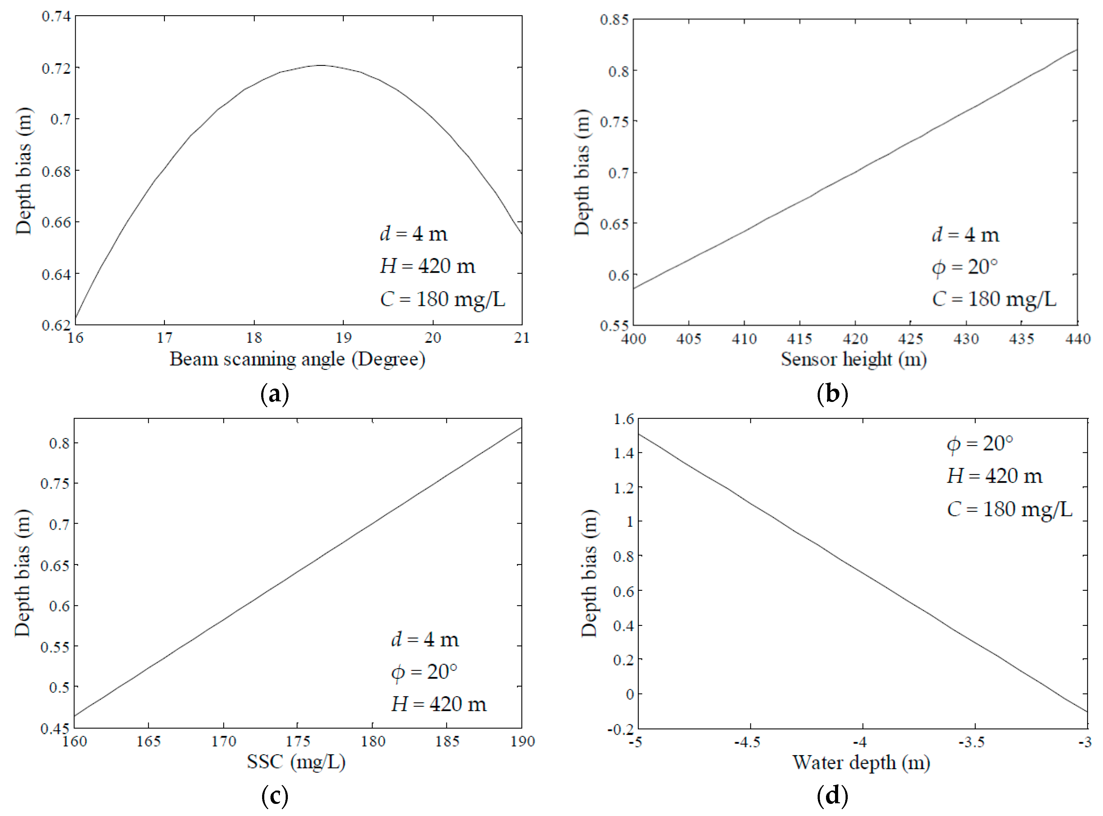
To accurately analyze the effects of the preceding parameters on depth bias, Equation (14) and the coefficients in the improved depth bias model were used to reflect the relationships of Δd varying with d, φ, H, and C. Figure 4 shows these relationships. In a relatively small range of φ, Δd increased with φ, whereas Δd decreased gradually with φ when φ increased to a certain range (Figure 4a). In terms of CZMIL instruments, the turning point of depth bias changing with the beam scanning angle appeared at φ as 18.8° when the water depth was 4 m, sensor height was 420 m, and SSC was 180 mg/L. This phenomenon can be explained by Guenther’s theory [2]. Two competing effects existed: path lengthening due to multiple scattering and path shortening due to energy returning early from the “undercutting” region [2]. The magnitudes of these effects depend strongly on the beam scanning angle [2]. The geometric dispersion effect, which causes path shortening, is dominant when the beam scanning angle is smaller than 18.8°. The multiple scattering effect, which causes path lengthening, is dominant when the beam scanning angle is larger than 18.8°. The influences of sensor height and SSC on depth bias exhibited a positive correlation (Figure 4b,c), namely, the depth biases increased with the two parameters. The larger the sensor height was, the larger the laser spot size and depth bias were. The larger the SSC was, the more expanded the laser beam was and the larger the depth bias was. Depth bias decreased linearly with water depth (Figure 4d), which is consistent with the actual measurement data shown in Figure 3d.
3.4. Accuracy Analysis
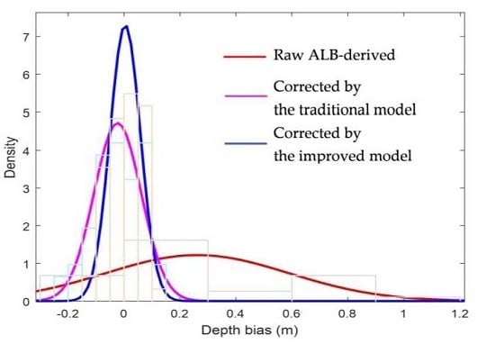
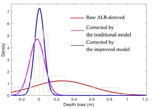
To evaluate the ALB depth bias models, the traditional depth bias model depicted in Equation (2) and the improved depth bias model depicted in Equation (14) were established with the 317 point pairs, respectively. The model coefficients and t-test results of the improved and traditional models are shown in Table 4 and Table 5, respectively. The raw ALB-derived depths of the remaining 62 point pairs were corrected by the two models and compared with the sounding data. The distributions of residual depth biases after correction varying with SSC are shown in Figure 5, and their statistical parameters and corresponding probability density functions are shown in Table 6 and Figure 6, respectively.
The “Order-1” specification of the International Hydrographic Organization (IHO) defines the maximum allowable total vertical uncertainty (TVU) at the 95% confidence level, which can be computed as follows:
where d is the water depth.
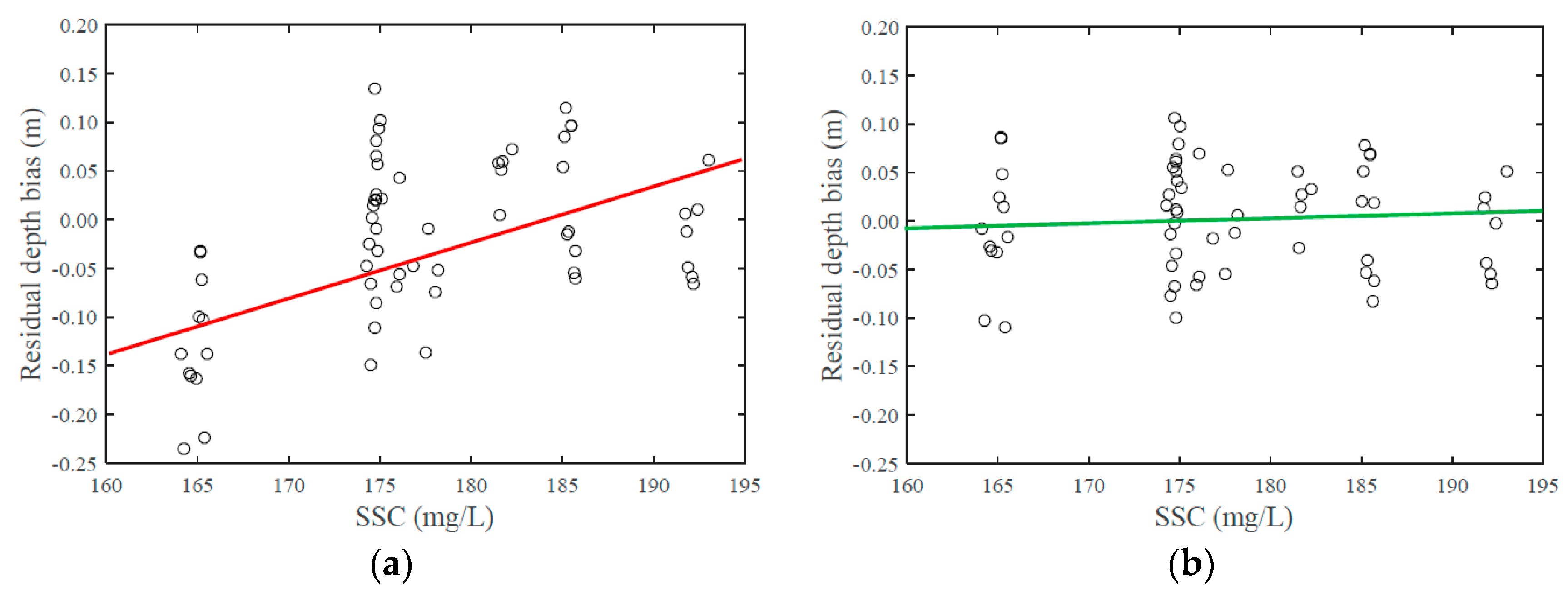
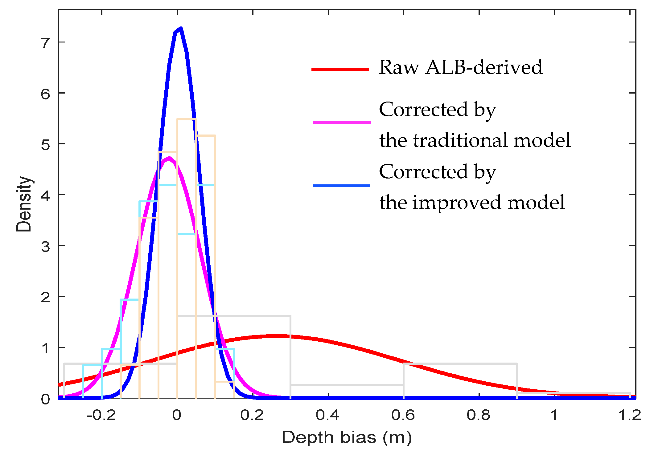
Using a method presented in previous literature [35], we used the mean bias plus twice the standard deviation as the worst case to determine if the correction results meet the accuracy standard of IHO. Table 6 and Figure 6 show that the raw ALB-derived depths had a maximum deviation of 1.173 m, standard deviation of 0.327 m, and systematic deviation of 0.262 m. The worst case was 0.916 m, which exceeds the maximum allowable TVU of 0.502 m when the water depth is 5 m and cannot meet the “Order-1” specification. The ALB depth corrected by the traditional and improved models exhibited a better accuracy than the raw ALB depth and can meet the “Order-1” specification. The systematic deviations weakened, and standard deviations of 0.086 and 0.055 m were obtained by the traditional and improved models, respectively. The accuracy of the ALB-derived depth corrected by the improved model was improved relative to that corrected by the traditional model. Moreover, Figure 5 shows that the depth biases corrected by the traditional model varied linearly with SSC, whereas those corrected by the improved model changed slightly with SSC. This result is due to disregarding SSC variation in the traditional depth bias model and considering SSC variation in the improved depth bias model.
4. Discussion
The proposed method provides a good means to reduce depth bias and obtain an accurate water depth by ALB. The following factors influence the applications and accuracies of the proposed method.
(a) Different ALB systems
ALB systems are categorized as integrated IR and green ALB systems and green ALB systems according to the lasers used [36,37,38,39]. For integrated IR and green ALB systems in which an additional IR laser is used to detect the water surface accurately, the improved depth bias model can be used directly to correct the ALB-derived depth. However, for green ALB systems, the primary IR laser is no longer used, and the green surface return cannot accurately represent the water surface [1,38,39]. The height models of green ALB systems proposed by Jianhu Zhao et al. [38] that consider near water surface penetration (NWSP) of the green laser should be used to correct the green water surface and water bottom heights. Then, the improved depth bias model can be used to correct the ALB-derived depth bias.
(b) Effects of surface wave and bottom slope
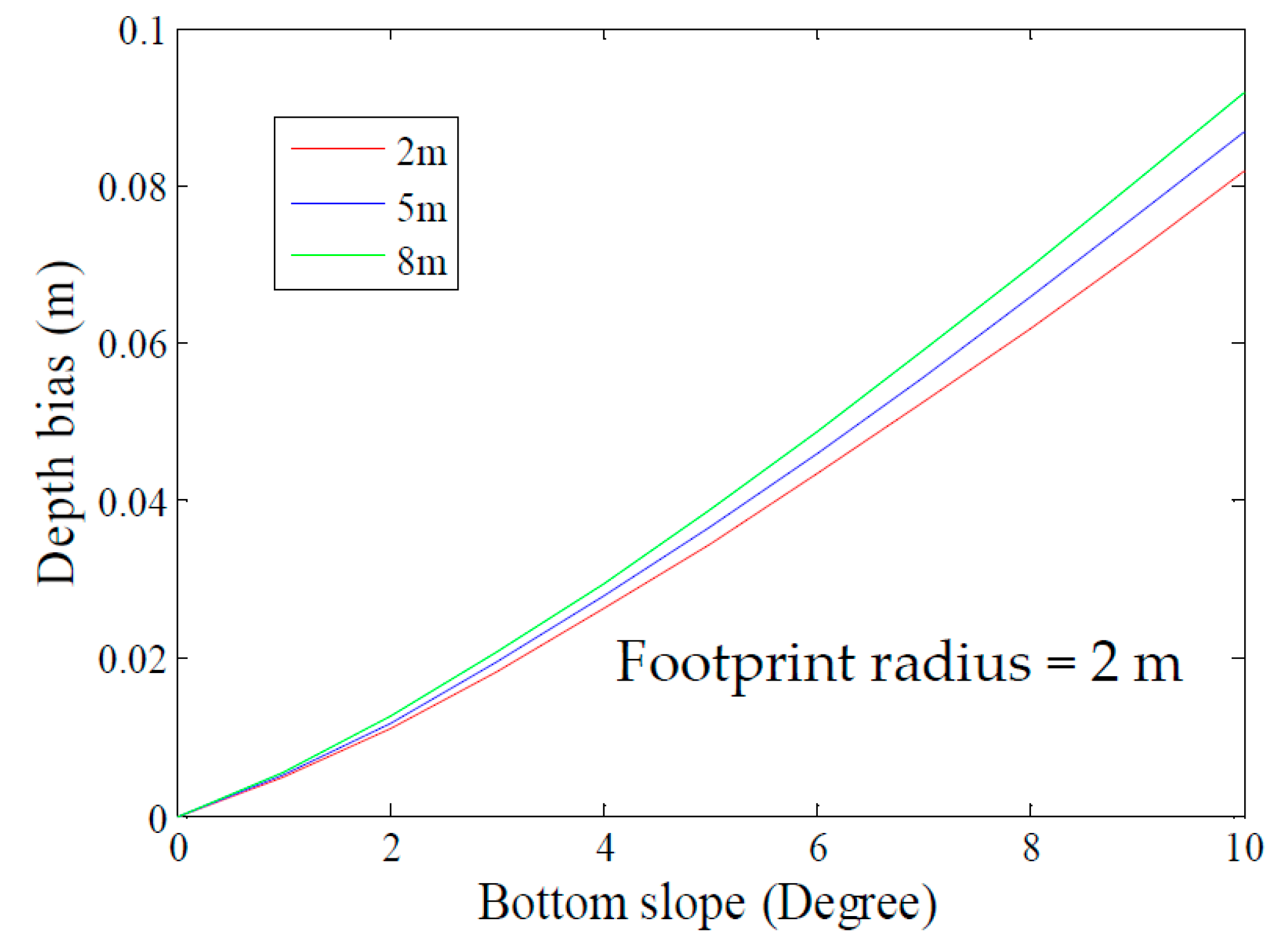
Surface wave and bottom slope affect ALB depth. As mentioned previously, the surface wave affects depth bias and is difficult to characterize and incorporate within a model [18]. The effect is not considered in the improved depth bias model but is weakened during data preprocessing. During data preprocessing, the slope of gravity waves can be estimated by referring to wave height and wavelength caused by wind speed, and its effect can be compensated for by adding the surface wave slope to the beam scanning angle when the laser beam footprint is incident on a single water surface facet or a single slope value. Capillary waves are small. Water surface with small capillary waves can be regarded as flat. The bottom slope can change the bottom incident angle of the laser beam and affect the pulse stretching of the green bottom return [14]. The larger the bottom slope is, the more the peak of the bottom return shifts to the surface return and the larger the depth bias is [14]. In reference [14], a model was proposed to estimate the effect of the bottom slope on ALB depth, and the effect varying with the bottom slope is shown in Figure 7. The effect intensifies with the increase in the bottom slope. If the limitation is set to 0.05 m, then the effect of the bottom slope less than 7° can be ignored when the beam footprint radius is less than 2 m and the water depth is less than 10 m; otherwise, the effect should be considered. By using the model proposed in reference [14], the effect can be estimated by integrating the beam footprint size, water depth, and bottom slope for the compensation of ALB depth. The residual of the compensation remains in the depth bias and should be further corrected by the improved model proposed in this study.
(c) Effects of flight directions
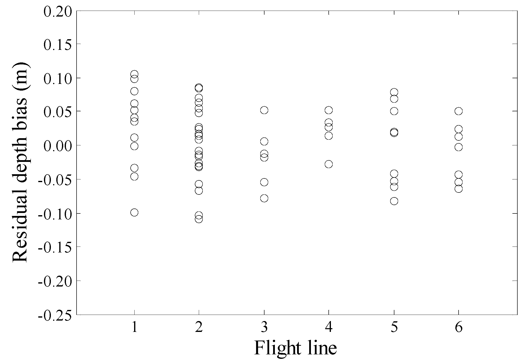
As shown in Figure 2, the flight directions of the six lines are different. Different flight directions change the relative location of the sensor to the sun, introduce various background noises in the pulse waveform, and affect the ALB depth measurements. The effect can be filtered before using a pulse detection algorithm [40]. Moreover, the effect of the surface wave on depth bias varies with flight directions [16]. The asymmetry of surface waves also plays an important role, affecting the return signal. It distorts the signal by altering the downwelling light field, complicating the comparison of the bottom return signals from two different flightlines. The asymmetry effects are less pronounced in strongly scattering environments making the effect less important in turbid waters or at greater depths [16]. Figure 8 shows the residual depth biases of the six flight lines in the red rectangular area in Figure 2. With the sounding result as a reference, the residual depth biases of different-direction flight lines were calculated by subtracting the reference from the ALB depth compensated for by the improved depth bias model. Standard deviations of 0.059 and 0.042 m were obtained by the northwest–southeast flight lines (lines 1, 2, and 5 in Figure 2) and the southeast–northwest flight lines (lines 3, 4, and 6), respectively. The residual of the northwest–southeast flight direction was slightly larger than that of the southeast–northwest flight direction. Large background noise may be introduced to the northwest–southeast direction ALB measurements because this direction is facing sunlight.
(d) Applications
The current experiment was conducted in a shallow water area with a water depth range of 3 to 4.5 m and SSC variation of 164 mg/L to 193 mg/L. The proposed improved model can correct the depth bias in this area. In other water areas with different water depths and turbidity, the depth bias model needs to be built according to the corresponding parameters of the measurement area used in Equation (6). The established depth bias model may be different from the above model in terms of model coefficients, but the modeling process and model form are the same as those depicted above.
5. Conclusions and Suggestions
An improved model for ALB depth bias correction was developed by considering ALB measurement and ocean hydrological parameters. The t-test of the model coefficient showed that all of the parameters in the improved model are significant and should be included, which indicates that the proposed improved model is reasonable. The traditional model and the proposed improved model were used to correct raw ALB-derived depth bias. The accuracies of ALB-derived depths corrected by the two models meet the “Order-1” specification of the IHO and have standard deviations of 0.086 and 0.055 m, respectively. The improved model is better than the traditional model.
In the application of the improved model, various factors, such as different ALB systems, surface waves, seabed slopes, and measurement areas, should be considered. The process of depth bias correction depicted in this study is appropriate for integrated IR and green ALB systems, but can be used for green ALB systems after calculating the water surface and water bottom heights considering the NWSP of the green laser. The surface wave effect can be estimated by referring to the wave height and can be compensated for by adding the surface wave slope to the beam scanning angle. The effect of the bottom slope can be estimated and compensated for by an approximation model. Although the modeling process and model form are suitable for other water areas, the depth bias model must be re-established by the local modeling parameters. The authors recommend using the traditional model in water areas with approximately the same turbidity and using the improved model in water areas with varying turbidity. In addition, density and representativeness should be considered in setting SSC sampling stations based on the measured water area to guarantee the accuracy of the proposed method.
Acknowledgments
This research is supported by the National Natural Science Foundation of China (Coded by 41376109, 41176068, and 41576107) and the National Science and Technology Major Project (Coded by 2016YFB0501703). The data used in this study were provided by the Survey Bureau of Hydrology and Water Resources of Yangtze Estuary. The authors are grateful for their support.
Author Contributions
Jianhu Zhao, Hongmei Zhang, and Xinglei Zhao developed and designed the experiments; Fengnian Zhou and Xinglei Zhao performed the experiments; Jianhu Zhao, Hongmei Zhang, and Xinglei Zhao analyzed the data; Jianhu Zhao, Hongmei Zhang, and Xinglei Zhao wrote the paper.
Conflicts of Interest
The authors declare no conflict of interest.
Appendix A
(1) t-test
To assess the reliabilities of the depth bias model parameters, a t-test was adopted to perform the hypothesis tests on the regression coefficients of the linear regression model. For the depth bias model, Δd is a dependent variable, xj is an independent variable, and βj is the partial regression coefficient of xj. Thereafter, the null hypothesis H0 and the alternative hypothesis H1 can be defined using the following equation:
where βj reflects the partial effect of xj on Δd after controlling for all of the other independent variables. Therefore, H0 indicates that xj does not affect Δd, which is called a significance test [41,42]. The statistic applied to test H0 against any alternative is called the t-statistic (t) and is expressed using the following equation:
where is the least squares estimate of and is the standard error of .
where n is the sample size, k is the number of estimated parameters, and ei is the residual.
The t-statistics calculated using Equation (A2) are compared with a theoretical t-distribution with n–k degrees of freedom. From the t-distribution, we obtain a probability (Prob. > |t|), called the p-value [42]. p-values (p) refer to the probability of the observed data or data to be more extreme, given that the null hypothesis is true, and the sampling is done randomly [43]. Once the p-value is determined, it can be compared with the given significance level α to determine whether to reject or not reject the null hypothesis [42]. For a typical analysis using the standard α = 0.05 cutoff, the null hypothesis is rejected when p < 0.05 and not rejected when p > 0.05.
If H0 is rejected, then xj is statistically significant at α, and the depth bias model indicates a linear relationship between xj and Δd. Otherwise, a linear relationship does not exist.
(2) Stepwise regression
Stepwise regression is an automated search procedure for selecting variables for a regression model; this procedure is beneficial when dealing with problems that involve multicollinearity [31]. Multicollinearity encompasses linear relationships between two or more variables [44], and can result in misleading and occasionally abnormal regression results [42]. If the p-values of nearly all model parameters are greater than α, then multicollinearity may be present in the model. Thus, the model should be optimized by stepwise regression. In stepwise regression, variables are added one at a time. The order of entry of the variables is controlled by a statistical program, and the variable that will lead to the largest increase in R2 is entered in each step. If an earlier variable becomes statistically insignificant with the addition of later variables, then such variables can be dropped from the model to prevent multicollinearity in the final regression model [42].
(3) IDW method
The SSC of all the sounding points can be interpolated as follows:
where n is the total number of sediment sampling stations, i = 1 − n is the ith sampling station, Pi is the weight of the ith sampling station, and Ci is SSC of the surface layer of the ith sampling station. The weight Pi is calculated as follows:
where Di is the distance from the sounding point to the ith sampling station, (x, y) is the plane coordinates of the sounding point, and (xi, yi) is the plane coordinate of the ith sampling station.
References
- Guenther, G.C.; Cunningham, A.G.; Laroque, P.E.; Reid, D.J. Meeting the accuracy challenge in airborne LiDAR bathymetry. In Proceedings of the 20th EARSeL Symposium: Workshop on LiDAR Remote Sensing of Land and Sea, Dresden, Germany, 16–17 June 2000. [Google Scholar]
- Guenther, G.C. Airborne Laser Hydrography: System Design and Performance Factors. Available online: http://shoals.sam.usace.army.mil/downloads/Publications/AirborneLidarHydrography.pdf (accessed on 25 February 2017).
- Guenther, G.C. Airborne LiDAR Bathymetry. Available online: https://pdfs.semanticscholar.org/a3a3/3880cd50e88b65f49c7c86e84526eaa3398d.pdf (accessed on 25 February 2017).
- Irish, J.L.; White, T.E. Coastal engineering applications of high-resolution LiDAR bathymetry. Coast. Eng. 1998, 35, 47–71. [Google Scholar] [CrossRef]
- Wang, C.; Li, Q.; Liu, Y.; Wu, G.; Liu, P.; Ding, X. A comparison of waveform processing algorithms for single-wavelength LiDAR bathymetry. ISPRS J. Photogramm. Remote Sens. 2015, 101, 22–35. [Google Scholar] [CrossRef]
- Quadros, N.D.; Collier, P.A.; Fraser, C.S. Integration of bathymetric and topographic LiDAR: A preliminary investigation. Int. Arch. Photogramm. Remote Sens. Spatial Inf. Sci. 2008, 36, 1299–1304. [Google Scholar]
- Wozencraft, J.; Millar, D. Airborne LiDAR and integrated technologies for coastal mapping and nautical charting. Mar. Technol. Soc. J. 2005, 39, 27–35. [Google Scholar] [CrossRef]
- Pittman, S.J.; Costa, B.M.; Battista, T.A. Using LiDAR bathymetry and boosted regression trees to predict the diversity and abundance of fish and corals. J. Coast. Res. 2009. [Google Scholar] [CrossRef]
- Cappucci, S.; Valentini, E.; Monte, M.D.; Paci, M.; Filipponi, F.; Taramelli, A. Detection of natural and anthropic features on small islands. J. Coast. Res. 2017, 77, 73–87. [Google Scholar] [CrossRef]
- Taramelli, A.; Valentini, E.; Innocenti, C.; Cappucci, S. FHYL: Field spectral libraries, airborne hyperspectral images and topographic and bathymetric LiDAR data for complex coastal mapping. In Proceedings of the Geoscience and Remote Sensing Symposium (IGARSS), Melbourne, Australia, 21–26 July 2013. [Google Scholar]
- Ramnath, V.; Feygels, V.; Kopilevich, Y.; Park, J.Y.; Tuell, G. Predicted bathymetric LiDAR performance of coastal zone mapping and imaging LiDAR (CZMIL). Proc. SPIE 2010, 7695, 769511. [Google Scholar]
- Penny, M.; Abbot, R.; Phillips, D.; Billard, B.; Rees, D.; Faulkner, D. Airborne laser hydrography in Australia. Appl. Opt. 1986, 25, 2046–2058. [Google Scholar] [CrossRef] [PubMed]
- Guenther, G.C.; Thomas, R.W. Error Analysis of Pulse Location Estimates for Simulated Bathymetric LiDAR Returns; NOAA Technical Report; University of California Libraries: Berkeley, CA, USA, 1981. [Google Scholar]
- Bouhdaoui, A.; Bailly, J.S.; Baghdadi, N.; Abady, L. Modeling the water bottom geometry effect on peak time shifting in LiDAR bathymetric waveforms. IEEE Geosci. Remote Sens. Lett. 2014, 11, 1285–1289. [Google Scholar] [CrossRef]
- Walker, R.E.; McLean, J.W. LiDAR equations for turbid media with pulse stretching. Appl. Opt. 1999, 38, 2384–2397. [Google Scholar] [CrossRef] [PubMed]
- Wang, C.K.; Philpot, W.D. Using airborne bathymetric LiDAR to detect bottom type variation in shallow waters. Remote Sens. Environ. 2007, 106, 123–135. [Google Scholar] [CrossRef]
- Thurman, H.V. Essentials of Oceanography; Merrill Publishing Company: Columbus, OH, USA, 1990. [Google Scholar]
- Billard, B.; Abbot, R.H.; Penny, M.F. Modeling depth bias in an airborne laser hydrographic system. Appl. Opt. 1986, 25, 2089–2098. [Google Scholar] [CrossRef] [PubMed]
- Wright, C.W.; Kranenburg, C.J.; Troche, R.J.; Mitchell, R.W.; Nagle, D.B. Depth Calibration of the Experimental Advanced Airborne Research LiDAR, EAARL-B.U.S.; Geological Survey Open-File Report 2016–1048; U.S. Geological Survey: Reston, VA, USA, 2016.
- Hilldale, R.C.; Raff, D. Assessing the ability of airborne LiDAR to map river bathymetry. Earth Surf. Process. Landf. 2008, 33, 773. [Google Scholar] [CrossRef]
- Skinner, K.D. Evaluation of LiDAR-Acquired Bathymetric and Topographic Data Accuracy in Various Hydrogeomorphic Settings in the Deadwood and South Fork Boise Rivers, West-Central Idaho, 2007; U.S. Geological Survey Scientific Investigations Report 2011-5051; U.S. Geological Survey: Reston, VA, USA, 2011.
- Abdallah, H.; Baghdadi, N.; Bailly, J.S.; Pastol, Y.; Fabre, F. Wa-LiD: A new LiDAR simulator for waters. IEEE Geosci. Remote Sens. Lett. 2012, 9, 744–748. [Google Scholar] [CrossRef]
- Gippel, C.J. Potential of turbidity monitoring for measuring the transport of suspended solids in streams. Hydrol. Process. 1995, 9, 83–97. [Google Scholar] [CrossRef]
- Lewis, J. Turbidity-controlled suspended sediment sampling for runoff-event load estimation. Water Resour. Res. 1996, 32, 2299–2310. [Google Scholar] [CrossRef]
- Grayson, R.; Finlayson, B.L.; Gippel, C.; Hart, B. The potential of field turbidity measurements for the computation of total phosphorus and suspended solids loads. J. Environ. Manag. 1996, 47, 257–267. [Google Scholar] [CrossRef]
- Smith, D.; Davies-Colley, R. If visual clarity is the issue then why not measure it. In Proceedings of the National Monitoring Conference, Madison, MA, USA, 19–23 May 2002. [Google Scholar]
- Mitchell, S.; Burgess, H.; Pope, D. Observations of fine-sediment transport in a semi-enclosed sheltered natural harbour (Pagham Harbour, UK). J. Coast. Res. 2004, 41, 141–147. [Google Scholar]
- Pavanelli, D.; Bigi, A. Indirect methods to estimate suspended sediment concentration: Reliability and relationship of turbidity and settleable solids. Biosyst. Eng. 2005, 90, 75–83. [Google Scholar] [CrossRef]
- Chanson, H.; Takeuchi, M.; Trevethan, M. Using turbidity and acoustic backscatter intensity as surrogate measures of suspended sediment concentration in a small subtropical estuary. J. Environ. Manag. 2008, 88, 1406–1416. [Google Scholar] [CrossRef] [PubMed]
- Carr, D.A. A Study of the Target Detection Capabilities of an Airborne LiDAR Bathymetry System. Ph.D. Thesis, Georgia Institute of Technology, Atlanta, GA, USA, 2013. [Google Scholar]
- Stepwise Regression. Available online: http://ncss.wpengine.netdna-cdn.com/wp-content/themes/ncss/pdf/Procedures/NCSS/Stepwise_Regression.pdf (accessed on 18 January 2017).
- Bartier, P.M.; Keller, C.P. Multivariate interpolation to incorporate thematic surface data using inverse distance weighting (IDW). Comput. Geosci. 1996, 22, 795–799. [Google Scholar] [CrossRef]
- Lawson, S.; Wiberg, P.; McGlathery, K.; Fugate, D. Wind-driven sediment suspension controls light availability in a shallow coastal lagoon. Estuar. Coasts 2007, 30, 102–112. [Google Scholar] [CrossRef]
- Wu, D.; Hu, G. Interpolation calculation methods for suspended sediment concentration in the yangtze estuary. In Proceedings of the IEEE International Conference on Intelligent Computing and Intelligent Systems, Shanghai, China, 20–22 November 2009. [Google Scholar]
- LaRocque, P.E.; Banic, J.R.; Cunningham, A.G. Design description and field testing of the SHOALS-1000T airborne bathymeter. Proc. SPIE 2004, 5412, 162–184. [Google Scholar]
- Alne, I.S. Topo-Bathymetric LiDAR for Hydraulic Modeling-Evaluation of LiDAR Data from Two Rivers. Master’s Thesis, Norwegian University of Science and Technology, Trondheim, Norway, 2016. [Google Scholar]
- Quadros, N.D. Unlocking the Characteristics of Bathymetric LiDAR Sensors. Available online: http://www.lidarmag.com/content/view/10159/199/ (accessed on 18 January 2017).
- Zhao, J.; Zhao, X.; Zhang, H.; Zhou, F. Shallow Water Measurements Using a Single Green Laser Corrected by Building a Near Water Surface Penetration Model. Remote Sens. 2017, 9, 426. [Google Scholar] [CrossRef]
- Mandlburger, G.; Pfennigbauer, M.; Pfeifer, N. Analyzing near water surface penetration in laser bathymetry—A case study at the River Pielach. In Proceedings of the ISPRS Annals of the Photogrammetry, Remote Sensing and Spatial Information Sciences, Antalya, Turkey, 11–13 November 2013. [Google Scholar]
- Wong, H.; Antoniou, A. One-dimensional signal processing techniques for airborne laser bathymetry. IEEE Trans. Geosci. Remote Sens. 1994, 32, 35–46. [Google Scholar] [CrossRef]
- Uriel, E. Hypothesis Testing in the Multiple Regression Model. Available online: http://ctu.edu.vn/~dvxe/econometrics/uriel_chapter4.pdf (accessed on 18 January 2017).
- Keith, T.Z. Multiple Regression and Beyond; Pearson Education: Upper Saddle River, NJ, USA, 2005. [Google Scholar]
- Miller, J. Statistical significance testing—A panacea for software technology experiments? J. Syst. Softw. 2004, 73, 183–192. [Google Scholar] [CrossRef]
- Hamilton, L.C. Regression with Graphics: A Second Course in Applied Statistics; Brooks/Cole Pub. Co.: Pacific Grove, CA, USA, 1992. [Google Scholar]
Figure 1.
Principle of ALB measurement. d is the water depth. Δd is the depth bias induced by peak shifting of the green bottom return. The red and green colors represent infrared (IR) and green lasers, respectively. (a) Waveform detections with IR and green lasers; (b) propagation ways of the two lasers and the bias induced by peak shifting of the green bottom return; t0–t3 denote the initial emission time of the laser pulse, round-trip time of the IR surface return, round-trip time of the actual received green bottom return distorted by the pulse stretching effect, and round-trip time of the ideal green bottom return, respectively.

Figure 2.
Locations and scopes of the different measurements. The yellow, green, and blue colors denote the land, bottom points of ALB, and bottom points of the sonar, respectively. The black triangles denote the locations of the three SSC sampling stations. The arrows denote the flight directions. In the red rectangular box, sonar sounding and ALB data compensated by the improved depth bias model are used to calculate the residual depth bias and analyze the effects of different flight directions on depth bias in Section 4.

Figure 3.
Depth bias ∆d obtained by comparing HBALB and HBSonar at the same location Equation (9) changes with different parameters. (a–d) denote depth biases changing with beam scanning angle, sensor height, SSC, and water depth, respectively.
Figure 3.
Depth bias ∆d obtained by comparing HBALB and HBSonar at the same location Equation (9) changes with different parameters. (a–d) denote depth biases changing with beam scanning angle, sensor height, SSC, and water depth, respectively.

Figure 4.
Regression curves of depth biases, ∆d, varying with ALB measurement and ocean hydrological parameters. ∆d varying with (a) beam scanning angle, (b) sensor height, (c) SSC, and (d) water depth exhibits a parabola, monotonically increases, monotonically increases, and monotonically decreases, respectively.

Figure 5.
Distributions of depth bias corrected by the (a) traditional and (b) improved models varying with SSC.
Figure 5.
Distributions of depth bias corrected by the (a) traditional and (b) improved models varying with SSC.

Figure 6.
Probability density function curves of the depth biases: raw ALB-derived, corrected by the traditional depth bias model, and corrected by the improved depth bias model.
Figure 6.
Probability density function curves of the depth biases: raw ALB-derived, corrected by the traditional depth bias model, and corrected by the improved depth bias model.

Figure 7.
Effect of the bottom slope on depth bias.

Figure 8.
Residual depth bias induced by different flight lines. Flight lines 1, 2, and 5 are from northwest to southeast, whereas lines 3, 4, and 6 are along the opposite flight direction.
Figure 8.
Residual depth bias induced by different flight lines. Flight lines 1, 2, and 5 are from northwest to southeast, whereas lines 3, 4, and 6 are along the opposite flight direction.


Table 1.
Main technical parameters of CZMIL.
| Parameters | Specifications |
|---|---|
| Operating altitude | 400 m (nominal) |
| Aircraft speed | 140 kts (nominal) |
| Pulse repetition frequency | 10 kHz |
| Circular scan rate | 27 Hz |
| Laser wavelengths | IR: 1064 nm; green: 532 nm |
| Maximum depth single pulse | 4.2/Kd (bottom reflectivity > 15%) |
| Minimum depth | <0.15 m |
| Bathymetric accuracy | (0.32 + (0.013d)2)½ m, 2σ |
| Horizontal accuracy | (3.5 + 0.05d) m, 2σ |
| Scan angle | 20° (fixed off-nadir, circular pattern) |
| Swath width | 294 m nominal |
Table 2.
Suspended sediment concentrations (SSC) of different sampling stations.
| Sampling Station | SSC (mg/L) |
|---|---|
| 1 | 315 |
| 2 | 122 |
| 3 | 134 |
Table 3.
Statistical parameters of the five-type data used in the modeling. Δd: depth bias; d: water depth; φ: beam scanning angle; H: sensor height; C: SSC.
Table 3.
Statistical parameters of the five-type data used in the modeling. Δd: depth bias; d: water depth; φ: beam scanning angle; H: sensor height; C: SSC.
| Δd (m) | d (m) | φ (°) | H (m) | C (mg/L) | |
|---|---|---|---|---|---|
| Max. | 1.22 | −3.1 | 20.8 | 440 | 193 |
| Min. | −0.16 | −4.6 | 16.3 | 394 | 164 |
| Mean | 0.16 | −3.4 | 19.1 | 420 | 177 |
| Std. | 0.29 | 0.3 | 1 | 11 | 5.8 |
Table 4.
Coefficients and t-test results of the initial and improved depth bias models. SE: standard error; t: t-statistics.
Table 4.
Coefficients and t-test results of the initial and improved depth bias models. SE: standard error; t: t-statistics.
| Item | Coefficient (Units) | Initial Model | Improved Model | ||||||
|---|---|---|---|---|---|---|---|---|---|
| Value | SE | t | p | Value | SE | t | p | ||
| d | β1 (1) | −2.66 × 10⁻¹ | 2.38 | −1.11 × 10⁻¹ | 0.9114 | 1.17 | 4.46 × 10⁻¹ | 2.62 | 0.0093 |
| φd | β2 (deg−1) | −8.99 × 10⁻² | 4.94 × 10⁻² | −1.82 | 0.0699 | −1.22 × 10⁻¹ | 4.50 × 10⁻² | −2.70 | 0.0073 |
| φ2d | β3 (deg−2) | 2.35 × 10⁻³ | 1.32 × 10⁻³ | 1.78 | 0.0766 | 3.24 × 10⁻³ | 1.21 × 10⁻³ | 2.68 | 0.0078 |
| Hd | β4 (m−1) | 2.31 × 10⁻² | 1.30 × 10⁻² | 1.79 | 0.0752 | ||||
| H2d | β5 (m−2) | −2.93 × 10⁻⁵ | 1.53 × 10⁻⁵ | −1.91 | 0.0577 | −1.75 × 10⁻⁶ | 3.34 × 10⁻⁷ | −5.23 | 0.0000 |
| Cd | β6 (mg−1·L) | −4.62 × 10⁻² | 1.74 × 10⁻² | −2.65 | 0.0084 | −2.95 × 10⁻³ | 4.15 × 10⁻⁴ | −7.12 | 0.0000 |
| C2d | β7 (mg−2·L2) | 1.24 × 10⁻⁴ | 4.98 × 10⁻⁵ | 2.49 | 0.0134 | ||||
| Constant | b (m) | −2.79 | 1.39 × 10⁻¹ | −20.09 | 0.0000 | −2.53 | 8.93 × 10⁻² | −28.37 | 0.0000 |
Table 5.
Coefficients and t-test results of the traditional depth bias model.
| Item | Coefficients | Value | SE | t | p |
|---|---|---|---|---|---|
| d | β | −8.3 × 10⁻¹ | 1.8 × 10⁻² | −44.7 | 0.0000 |
| Constant | b | −2.6 | 6.3 × 10⁻² | −42.0 | 0.0000 |
Table 6.
Statistical parameters of the depth biases: raw ALB-derived, corrected by the traditional depth bias model, and corrected by the improved depth bias model.
Table 6.
Statistical parameters of the depth biases: raw ALB-derived, corrected by the traditional depth bias model, and corrected by the improved depth bias model.
| Depth Bias (m) | Max. | Min. | Mean | Std. | Worst Case | Meets IHO Standard |
|---|---|---|---|---|---|---|
| Raw ALB-derived | 1.173 | −0.167 | 0.262 | 0.327 | 0.916 | × |
| Corrected by the traditional model | 0.134 | −0.235 | −0.023 | 0.086 | 0.195 | √ |
| Corrected by the improved model | 0.106 | −0.109 | 0.004 | 0.055 | 0.114 | √ |
© 2017 by the authors. Licensee MDPI, Basel, Switzerland. This article is an open access article distributed under the terms and conditions of the Creative Commons Attribution (CC BY) license (http://creativecommons.org/licenses/by/4.0/).
Share and Cite
MDPI and ACS Style
Zhao, J.; Zhao, X.; Zhang, H.; Zhou, F. Improved Model for Depth Bias Correction in Airborne LiDAR Bathymetry Systems. Remote Sens. 2017, 9, 710. https://0-doi-org.brum.beds.ac.uk/10.3390/rs9070710
AMA Style
Zhao J, Zhao X, Zhang H, Zhou F. Improved Model for Depth Bias Correction in Airborne LiDAR Bathymetry Systems. Remote Sensing. 2017; 9(7):710. https://0-doi-org.brum.beds.ac.uk/10.3390/rs9070710
Chicago/Turabian StyleZhao, Jianhu, Xinglei Zhao, Hongmei Zhang, and Fengnian Zhou. 2017. "Improved Model for Depth Bias Correction in Airborne LiDAR Bathymetry Systems" Remote Sensing 9, no. 7: 710. https://0-doi-org.brum.beds.ac.uk/10.3390/rs9070710
Note that from the first issue of 2016, this journal uses article numbers instead of page numbers. See further details here.