Mathematical Modeling and Accuracy Testing of WorldView-2 Level-1B Stereo Pairs without Ground Control Points

Abstract

With very high resolution satellite (VHRS) imagery of 0.5 m, WorldView-2 (WV02) satellite images have been widely used in the field of surveying and mapping. However, for the specific WV02 satellite image geometric orientation model, there is a lack of detailed research and explanation. This paper elaborates the construction process of the WV02 satellite rigorous sensor model (RSM), which considers the velocity aberration, the optical path delay and the atmospheric refraction. We create a new physical inverse model based on a double-iterative method. Through this inverse method, we establish the virtual control grid in the object space to calculate the rational function model (RFM) coefficients. In the RFM coefficient calculation process, we apply the correcting characteristic value method (CCVM) and least squares (LS) method to compare the two experiments’ accuracies. We apply two stereo pairs of WV02 Level 1B products in Qinghai, China to verify the algorithm and test image positioning accuracy. Under the no-control conditions, the monolithic horizontal mean square error (RMSE) of the rational polynomial coefficient (RPC) is 3.8 m. This result is 13.7% higher than the original RPC positioning accuracy provided by commercial vendors. The stereo pair horizontal positioning accuracy of both the physical and RPC models is 5.0 m circular error 90% (CE90). This result is in accordance with the WV02 satellite images nominal positioning accuracy. This paper provides a new method to improve the positioning accuracy of the WV02 satellite image RPC model without GCPs.

1. Introduction

Currently, rapid technological development of very high resolution satellites (VHRS) has increased commercial high-resolution optical satellite imagery resolution from 1 m to 0.3 m, showing enormous value in the field of surveying and mapping. Using a VHRS image, one can quickly obtain fundamental geographic information, such as digital elevation models (DEM), digital orthophoto maps (DOM), and digital line graphics (DLG), which have become some of the primary results of data collection. Before using the image for various applications, we must first build the correct geometric model based on the imaging principle of the satellite sensor. Currently, optical VHRS often use linear charge-coupled device (CCD) push-broom sensors to obtain images. Satellite linear array push-broom imaging differs from aerial images, with special characteristics, such as high flight altitude, a photographically narrow beam, and a small viewing angle [1]. There are two types of satellite geometric positioning models: the rigorous sensor model (RSM), also called the physical or camera model, and the rational function model (RFM).

Each of the scanning lines of the linear array CCD image is center projected, and the RSM reconstructs the photographic light beam based on this characteristic, establishing the collinearity condition and formulas [2] for geometric positioning. Toutin [3] proposed a 3D positioning method and a variety of sensors, such as the SPOT series, EROS A, QuickBird, and IKONOS, and has successful experimented with this model, which has been integrated into commercial software (PCI Geomatics). Crespi and Giannone [4,5,6,7] developed a physical model that was integrated into the SISAR software package and successfully used for EROS A, QuickBird, and other satellite data. BAE Systems’ software utilized by De Venecia et al. [8] uses a physical model to process ORBVIEW-3 data. We can summarize the characteristics of these models as follows: both are based on collinear formulas; both require the sensor parameters; the parameters of the model have a physical meaning; and the solution model of all parameters requires a certain ground control point. Since each VHRS metadata format and definition is different, there is no uniform physical model.

After the IKONOS satellite launched in 1999, the RFM became the mainstream image-processing model. In the beginning, RFM research primarily focused on the rational function model structure, the solution method of rational polynomial coefficients (RPCs), and the RFM precision. Tao and Hu [9,10,11] used aerial imagery, SPOT images, and IKONOS images to explore the collinear formula, two-dimensional and three-dimensional polynomial, perspective projection, and RFM correction methods differently. They found that the RFM correction method does not require sensor information and azimuth parameters, but has precision slightly worse than the collinear formulas. Cheng and Toutin [12] studied IKONOS geo-level images with the simple polynomial, rational function model, and the precision of the model, and the experimental results show that the positioning accuracy of the physical model is better than the other two effects. Yang [13] experimented on SPOT images showing that the RFM of the third-order, and even the second-order, denominator can replace the physical model. Grodecki and Dial’s [14,15,16] experiments on IKONOS images show that the RFM can be an alternative to the physical model, whose accuracy reaches the sub-pixel level even in the case of poor geometric conditions, verifying the RFM’s mapping capability and three-dimensional reconstruction in urban or mountainous areas.

Tao and Hu [9,10] studied the least squares principle to solve the calculation method of the RPCs and found that the correlation of RPCs leads to a singularity of the parameter array. Moreover, the regularization method can improve the number of design matrix conditions to avoid the least squares adjustment on the value of instability. They fit the physical model based on different forms of the RFM model and use the least squares and ridge estimations to calculate the RPC parameters. The experimental results show that the least squares estimation has the highest fitting accuracy, and the ridge estimation can obtain the RPC parameters with good structure (high-order terms close to zero) [17,18]. Qin et al. [19] proposed an algorithm of RPC parameters based on a global DEM without an initial value and, using a physical model to calculate the RPC parameters, the algorithm has been successfully tested with SPOT imagery.

In October 2009, DigitalGlobe (DG) launched a second WorldView series satellite, WorldView-2 (WV02). WV02 performance has improved significantly compared with WorldView-1, adding four standard multi-spectral bands of R, G, B, and NIR, and four new bands of Coast, Yellow, Red, and NIR2. DigitalGlobe is the world’s first company to provide an eight-band multi-spectral commercial remote sensing satellite. WV02 operates at 770 km in a sun synchronous orbit, with a panchromatic resolution of 0.46 m, and a multi-spectral resolution of 1.85 m at nadir. The specification horizontal geolocation accuracy CE90 (90% of circular error) and vertical accuracy (90% of linear error) is 5 m, while the mean square error (RMSE) is 2.3 m [20]. This accuracy is due to the direct sensor orientation without using any ground control points (GCPs), and with an off-nadir angle less than 30°, excluding terrain effects [21]. Recent studies have shown that the actual positioning accuracy of the WV02 satellite is better than the declared accuracy of 1–2 m. Readers can obtain more detailed information from Aguilar et al. [22,23] and David et al. [24].

The WV02 sensors use a push-boom scanner and the Basic Level-1B (L1B) image products provide a physical model and the RFM of two sets of parameters, but the commercial vendor did not provide their specific method of applying the physical model. If the users have an accurate physical model, the use of image metadata may improve RPC accuracy without GCPs. Currently, the research on this aspect is also inadequate. Therefore, it is necessary to invert the exact physical model according to the characteristics of the L1B image support document (ISD) and explore the method of improving the accuracy of the RFM under uncontrolled conditions.

In this paper, we focus on the construction of the physical model of the L1B image of the WV02 satellite under uncontrolled conditions and the calculation method of the coefficient of the RFM, which includes three main aspects:

• Based on the characteristics of the WV02 ISD file, we develop the precise physical model of the WV02 satellite.
• We establish a new inverse transform method from the physical model, calculate the object virtual control points, and convert them into image coordinates.
• To overcome the problem of the morbidity normal formula in the process of solving for the RPC coefficients, we iterate using the correcting characteristic value method and compare these results with the least squares results.

2. Description of the WV02 L1B Dataset and Study Area

2.1. Characteristics of the WV02 L1B Image Products

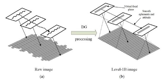
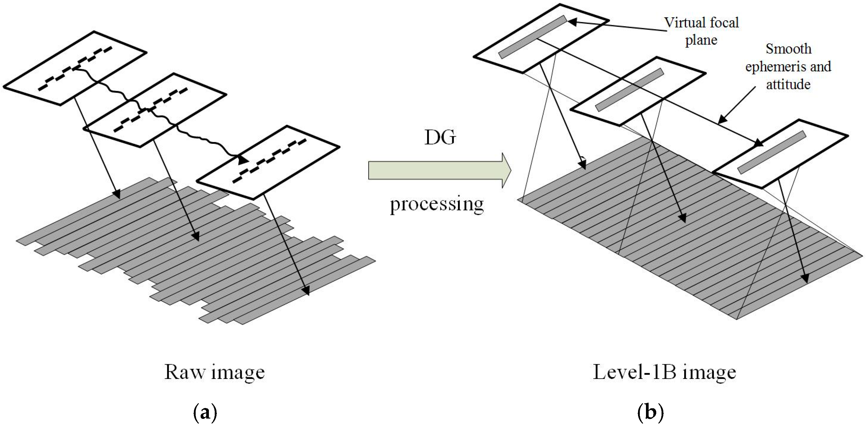
Due to manufacturing CCD size constraints, push-broom satellite detectors usually stitch together a plurality of CCDs to obtain a larger scan width. The WV02 satellite sensor uses time delay integration (TDI) technology. The panchromatic focal plane uses 50 panchromatic sub-sensors in the center of the detector, and the multi-spectral focal plane installations on both sides of the panchromatic focal plane each contain more than 10 sub-spectral sensors [25]. According to photogrammetry theory, to determine the position of the object, one must first obtain the line of sight (LOS) direction element, which contains the interior orientation (IO) and exterior orientation (EO) parameters. We can obtain the relationship between each CCD probe and the sensor focal plane inside the camera from the ground and aerial calibrations, and the positional relationship between the satellite sensor and the satellite body. That is, the azimuth element of the sensor, provided by a geometric calibration file (*.GEO) file. The outer orientation elements of each images’ scan line are obtained by star tracker cameras and on-board GPS receivers, which can be interpolated by ephemeris (*.EPH) and attitude files (*.ATT). By filtering the ephemeris and position, and by generating a regular virtual scan line, we can resample the original image to obtain an image conforming to the ideal conformational condition. The process of the satellite acquiring the raw image and transferring it into the L1B image is shown in Figure 1. The L1B image did not provide any map projection; it is only conducting a radiation and sensor correction from the original image. The L1B image is the closest product to the raw image. As the attitude and satellite position changes slowly, resulting in a slow LOS direction change, each pixel resolution ground sample distance (GSD) is different after resampling.

In fact, in the process of image acquisition, each CCD probe has a tight imaging relationship; the image resampling will break the collinear relationship of the original image and the objective points. Users must understand the correlation between the original image and the L1B image, or resampling method, to re-establish a strict L1B image physical model. For example, SPOT imagery provides a level-1A image to level-1B image conversion polynomial. However, because DG does not provide the original image, it has not published its algorithm to establish the physical model. Therefore, it is necessary to model the WV02 satellite imaging geometry based on the content of the ISD files and the push-broom scanner rule.

2.2. Study Area and Dataset

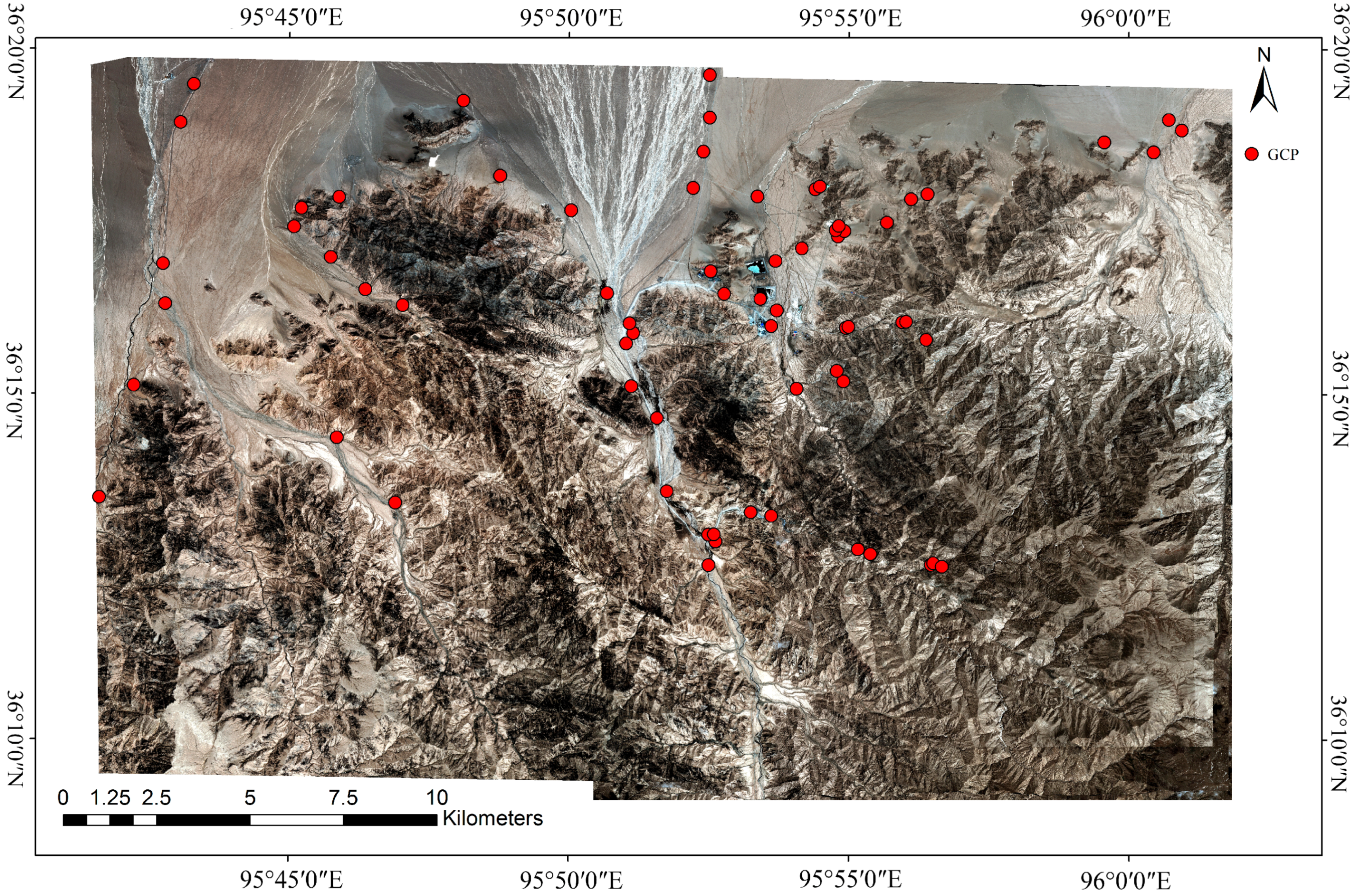
The study area is located in western China, the Qinghai-Tibet Autonomous Region, on the northern slope of the Kunlun Mountains, in an area of approximately 400 km² (Figure 2). The coordinates of the study area are UTM zone 46 N ellipsoid WGS84. The study area is complex and dangerous terrain, containing steep mountains, with elevations between 3000 m and 4300 m, and a relative height difference of 300–1000 m. The test area image data are two along-track stereo pairs of WV02 L1B products.

Table 1. Details of the WorldView-2 basic (L1B) stereo pairs in the study area.

Product Order ID	054471964010_01		054471964020_01
Product Name	15JUL10043733-	15JUL10043857-	15JUL24042129-	15JUL24042233-
Generation Time (UTC)	10 July 2015 T07:04:36	10 July 2015 T07:05:08	24 July 2015 T06:03:26	24 July 2015 T06:04:03
Num Rows × Num Columns	27,164 × 34,584	24,356 × 35,180	22,716 × 35,180	28,048 × 34,445
Scan Direction	Forward	Forward	Forward	Forward
Mean Product GSD (m)	0.516	0.553	0.649	0.518
Satellite Azimuth Angle	350.000	210.500	40.300	97.400
In Track View Angle (°)	16.600	–23.000	27.700	0.600
Cross Track View Angle (°)	–6.500	–8.700	18.800	17.600
Off Nadir View Angle (°)	17.800	24.500	33.100	17.600
Cloud Cover (%)	0.005	0.006	0.000	0.000

lists the image parameters.

To verify the image geolocation accuracy, we use the GPS measurement method in the study area, and establish 75 ground control points as independent checkpoints (ICPs). The ICP are outstanding points, properly selected to determine the locations of the objects, such as roads, houses, or other independent objects. These points can be accurately identified in both photos and on the ground. The ICP distribution is shown in Figure 3. The survey error in these control points is less than 5 cm both in the horizontal and vertical directions; the pointing error is less than 1 pixel (0.5 m).

3. The Physical Model of WV02

3.1. Calculation Principle

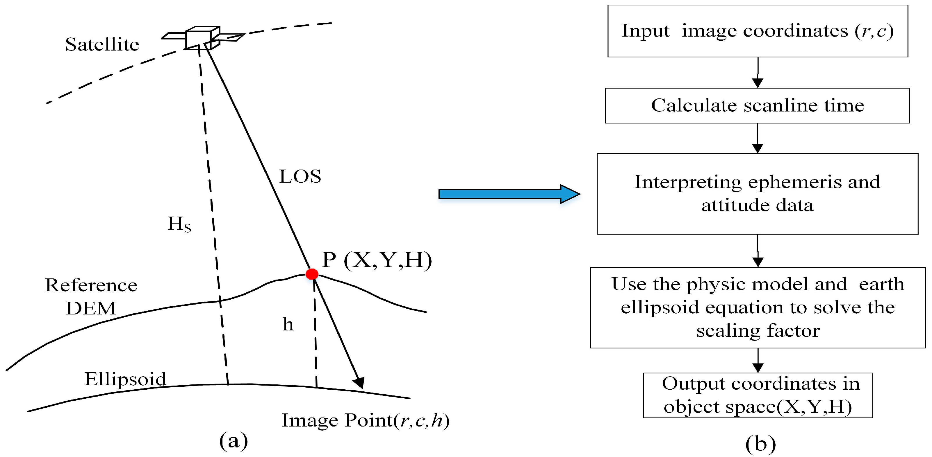
For a linear array CCD sensor, the strict geometric model of the direct positioning algorithm and process are almost identical. We can describe the satellite sensor imaging process as a series of spatial coordinate transformations of the LOS direction to determine the location of a point in Earth-centered, Earth-fixed (ECEF) coordinates. Figure 4 shows the spatial coordinate transformation process.

The physical model recovery LOS, based on the principle of collinear formulas, has two positioning methods: monolithic and stereoscopic. Monolithic positioning requires high-precision DEM support. The positioning process first calculates the line scan time based on the image coordinates. Using this time value, the ephemeris and attitude data are interpolated to obtain the outer azimuth elements and to combine the sensor inner azimuth elements. Finally, the LOS direction is retrieved to determine the intersection of the LOS and the Earth’s ellipsoid surface. Figure 5a shows the positioning principle and the calculation process. In the direct positioning solution, one must read the basic motion vector, attitude parameters, geometric calibration parameters, and other data in the image metadata file. These image support data are provided by DG for basic imagery. The direct location process to calculate Point P(r, c) is shown in Figure 5b, using only the signal image.

We can summarize the general physical mode for most linear array push-broom satellites as follows:

$${\left[\begin{array}{c}X\\ Y\\ Z\end{array}\right]}_{WGS84}={\left[\begin{array}{c}{X}_{GPS}\\ Y_{GPS}\\ Z_{GPS}\end{array}\right]}_{WGS84}+R_{{}_{J2000}}^{{}^{WGS84}}{R}_{body}^{{}^{J2000}}\left(\left[\begin{array}{c}{D}_X\\ D_Y\\ D_Z\end{array}\right]+\left[\begin{array}{c}{d}_X\\ d_Y\\ d_Z\end{array}\right]+\lambda R_{{}_{camera}}^{body}{\left[\begin{array}{c}X\\ Y\\ Z\end{array}\right]}_{camera}\right)$$

(1)

where ${\left[XYZ\right]}_{WGS84}^T$ is P’s ECEF (WGS84) coordinate, and ${\left[X_{GPS}{Y}_{GPS}{Z}_{GPS}\right]}_{WGS84}^T$ is the GPS antenna phase center. ${\left[d_X{d}_Y{d}_Z\right]}_{WGS84}^T$ is the origin translation of the camera coordinate to the satellite body system, and ${\left[XYZ\right]}_{camera}^T$ is the coordinate of the ground point P in the camera system. $R_{{}_{J2000}}^{{}^{WGS84}}$ is the rotation matrix of the J2000 coordinate system to ECEF(WGS84). $R_{body}^{{}^{J2000}}$ is the rotation matrix of the satellite body system to the J2000 coordinate system. $R_{{}_{camera}}^{body}$ is the rotation matrix of the satellite camera system to the satellite body system.

3.2. Simplification of the Physical Model

Based on the characteristics of the WV02 image support file, we further simplified Equation (1) as follows:

$${\left[\begin{array}{c}X\\ Y\\ Z\end{array}\right]}_{camera}=R_{focal\_plane}^{\det ector}\left[\begin{array}{c}0+x_0\\ -y_i+y_0\\ f\end{array}\right]$$

(2)

where the following:

$$R_{focal\_plane}^{\det ector}=\left[\begin{array}{ccc}\cos \gamma & \sin \gamma & 0\\ -\sin \gamma & \cos \gamma & 0\\ 0& 0& 1\end{array}\right]$$

(3)

and $R_{focal\_plane}^{\det ector}$ is the rotation matrix of the line array detector system to the camera system. The angle between the detector and the camera system z-axis is γ, which is the “detRotAngle” parameter in the GEO file. ${[x_0-y_i+y_{0}f]}^T$ is the ground point P coordinate in the instantaneous image system. $(x_0,y_0)$ is the offset between the center of the first pixel (0, 0) and the origin of the camera coordinate system. We can obtain these data from the GEO file. In Equation (1), $R_{J2000}^{WGS84}{R}_{body}^{J2000}$ represents the conversion from the satellite body system to the orbital coordinate system and the orbital coordinate system to the WGS84 system. Then, we can write the following:

$$R_{J2000}^{WGS84}{R}_{body}^{J2000}=R_{body}^{WGS84}$$

(4)

After geometric correction and resampling of the WV02 satellite raw image, we can consider that the GPS antenna phase center and the satellite body center are coincident and that the camera center and the satellite body center also coincide. Therefore, we have ${[D_X{D}_Y{D}_Z]}^T=0\mathrm{and}{[d_X{d}_Y{d}_Z]}^T=0$, and can simplify Equation (1) as the following:

$${\left[\begin{array}{c}X\\ Y\\ Z\end{array}\right]}_{WGS84}={\left[\begin{array}{c}{X}_{GPS}\\ Y_{GPS}\\ Z_{GPS}\end{array}\right]}_{WGS84}+\lambda R_{body}^{WGS84}{R}_{camera}^{body}{R}_{\det ector}^{camera}\left[\begin{array}{c}0+x_0\\ -y_i+y_0\\ f\end{array}\right]$$

(5)

In Equation (5), ${\left[X_{GPS}{Y}_{GPS}{Z}_{GPS}\right]}_{WGS84}^T$ is obtained through the ephemeris file (*.EPH) interpolation, and λ is the unsolved scaling factor. $R_{body}^{WGS84}$ is the rotation matrix of the satellite body system to the WGS84 system. We can construction this rotation matrix as Equation (6).

$$R=\left[\begin{array}{ccc}{q}_1^2-q_2^2-q_3^2+q_4^2& 2(q_1{q}_2-q_3{q}_4)& 2(q_1{q}_3+q_2{q}_4)\\ 2(q_1{q}_2+q_3{q}_4)& -q_1^2+q_2^2-q_3^2+q_4^2& 2(q_2{q}_3-q_1{q}_4)\\ 2(q_1{q}_3-q_2{q}_4)& 2(q_2{q}_3+q_1{q}_4)& -q_1^2-q_2^2+q_3^2+q_4^2\end{array}\right]$$

(6)

where (q₁,q₂,q₃,q₄) is the quaternion parameter which can be interpolated from the *.ATT file.

In Equation (5), the rotation matrix of the camera system and the body system is constructed by the image geometry correction file (*.GEO file). Based on Equation (6), this rotation matrix is stable for a long time after the satellite calibration. We can consider this rotation matrix to be a constant array. Let the rotation matrix $R={\left[R_{\det ector}^{camera}\right]}^T{\left[R_{camera}^{body}\right]}^T{\left[R_{body}^{WGS84}\right]}^T$, then Equation (5) can be rewritten as Equation (7).

$${\left[\begin{array}{c}X\\ Y\\ Z\end{array}\right]}_{WGS84}={\left[\begin{array}{c}{X}_{GPS}\\ Y_{GPS}\\ Z_{GPS}\end{array}\right]}_{WGS84}+\lambda R^T\left[\begin{array}{c}0+x_0\\ -y_i+y_0\\ f\end{array}\right]$$

(7)

Let $P_E(t)={\left[XYZ\right]}_{WGS84}^T$ and $S_E(t)={\left[X_{GPS}{Y}_{GPS}{Z}_{GPS}\right]}_{WGS84}^T$, then the following:

$$u=\left[\begin{array}{c}{u}_x\\ u_y\\ u_z\end{array}\right]=R^T\times \left[\begin{array}{c}0+x_0\\ -y_i+y_0\\ f\end{array}\right]$$

(8)

We can rewrite Equation (7) as follows:

$$P_E=S_E(t)+\lambda \overrightarrow{u},\overrightarrow{u}=u/\Vert u\Vert$$

(9)

where P_E is the point location in the object coordinates, S_E(t) is the sensor projection center position at time “t“, λ is the scale factor, and $\overrightarrow{u}$ is the unit vector of the LOS. Further, we can express Equation (9) in component form as follows:

$$\{\begin{array}{l}{X}_E=X_{E(t)}+\lambda \cdot {\overrightarrow{u}}_x\\ Y_E=Y_{E(t)}+\lambda \cdot {\overrightarrow{u}}_y\\ Z_E=Z_{E(t)}+\lambda \cdot {\overrightarrow{u}}_z\end{array}$$

(10)

Consider the following Earth ellipsoid formula:

$$\frac{X_E^2+Y_E^2}{{(a+h)}^2}+\frac{Z_E^2}{{(b+h)}^2}=1$$

(11)

where a = 6,378,137.0 m and b = 6,356,752.3 m are the long and the short axes of the WGS84 reference ellipsoid, and h is the point ellipsoid elevation. We can calculate λ by using Equations (10) and (11) and then obtain the ground coordinates in Equation (10). By using DEM data (such as SRTM data), we can obtain the elevation value h. The solution process is an iterative process (see “SPOT 123-4-5 Geometry Handbook” [26] for details).

3.3. Exterior Orientation (EO) Parameter Interpolation

In Section 3.1, we must interpolate the ephemeris and quaternion data using the following method.

3.3.1. Ephemeris Interpolation

The precision ephemeris file records the spatial position of the satellite’s GPS receiver at a certain frequency (50 Hz for WV02). To obtain the satellite position at any given time, we must interpolate our fitted ephemeris data. Commonly used mathematical methods include linear interpolation, Lagrangian polynomial interpolation, cubic spline interpolation, Chebyshev fitting, and general polynomial fitting. Under normal circumstances, for remote sensing satellite platforms in space to run more smoothly, these interpolations or fit methods can achieve a high accuracy. In this paper, we use Chebyshev fitting [27] for satellite position and velocity, and its mathematical model is described below.

Assume the satellite ephemeris data in time intervals $\left[t_0,t_0+\Delta t\right]$ can use an nth order Chebyshev polynomial fitting function, where $t_0$ is the start epoch and $\Delta t$ is the fitting time interval. First, convert the variables $t\in \left[t_0,t_0+\Delta t\right]$ to $\tau \in \left[-1,+1\right]$, where $\tau =\frac{2}{\Delta t}\left(t-t_0\right)-1,t\in \left[t_0,t_0+\Delta t\right]$. We can calculate the satellite location at any time t by using Equation (12).

$$\begin{array}{l}X(t)={\displaystyle \sum _{i=0}^n{C}_{Xi}{T}_i(\tau )}\\ Y(t)={\displaystyle \sum _{i=0}^n{C}_{Yi}{T}_i(\tau )}\\ Z(t)={\displaystyle \sum _{i=0}^n{C}_{Zi}{T}_i(\tau )}\end{array}\}$$

(12)

where n is the order of the Chebyshev polynomial and the Chebyshev polynomial coefficients of the coordinates are the following:

$$\begin{array}{l}{T}_0(\tau )=1,\\ T_1(\tau )=\tau ,\\ T_n(\tau )=2\tau T_{n-1}(\tau )-T_{n-2}(\tau );\left|\tau \right|\le 1,n\ge 2\end{array}\}$$

(13)

Based on the ephemeris file, we can find a number of $m(m>n+1)$ satellite coordinates in the range $\left[t_0,t_0+\Delta t\right]$ using the least squares method to find the Chebyshev polynomial coefficient $C_{Xi},C_{Yi},C_{Zi}(i=0,1,2,\cdots ,n)$. Then, we can calculate satellite coordinates by using Equation (11). The fitting method for the satellite’s velocity is similar.

3.3.2. Attitude Quaternion Interpolation

Currently, the majority of satellite image manufacturers use quaternions to express satellite attitude. Compared with the Euler angle, quaternions have some advantages, such as calculation speed, reduced storage space, and lack of singularity. The WV02 satellite attitude file provides satellite attitude data recorded at a 50 Hz frequency, and we can interpolate or fit these data to obtain the attitude data at any time point. The quadrature interpolation methods include linear and spline interpolation. In this paper, we use the spherical linear interpolation (SLERP) method [28]. The vector rotation quaternion mathematical definition is as follows:

$$q=q_0+q_{1}i+q_{2}j+q_{3}k$$

(14)

Equation (14) shows the mathematical model of the spherical interpolation, which shows that the direction of the vector is in the direction of interpolation in the rotation process.

$$q=\frac{\sin \left(\left(1-t\right)\omega \right)}{\sin \omega }{q}_a+\frac{\sin \left(t\omega \right)}{\sin \omega }{q}_b$$

(15)

where ω is the angle between q_a and q_b, which can be calculated as follows:

$$\omega =arc\cos \left(q_a\cdot q_b\right)$$

(16)

3.4. WV02 Satellite Physical Model Refinement

Using the general physical model established in Section 3.2, we found the WV02 location error to be large during experiments. Through experimental analysis, we determined the physical model of WV02 requires further refinement. The purpose of this refinement is to correct the direction of the LOS based on the ISD file provided by DG. These corrections include velocity aberration, speed of light delay, and atmospheric refraction. The specific process is shown in Figure 6.

3.4.1. Velocity Aberration Correction

A satellite sensor in the process of scanning, due to the impact of the Earth’s angular velocity, results in the subject of the moving direction (trajectory line) and the sub-satellite track direction (heading line) being inconsistent, resulting in velocity aberration. The calculation of velocity aberration is as follows:

• The velocity vector at a ground point is as follows:

  $${\overrightarrow{v}}_g=\overrightarrow{E}\times {\overrightarrow{P}}_E$$

  (17)

  where $\overrightarrow{E}$ is the Earth’s angular velocity vector, $\overrightarrow{E}={\left[00{\mathsf{\Omega }}_e\right]}^T$ and ${\mathsf{\Omega }}_e$ is the Earth’s angular velocity, ${\mathsf{\Omega }}_e=2\pi /T$, $T=86164.0905″$.
• Calculate the camera speed component that is orthogonal to the LOS as follows:

  $$\overrightarrow{v_{\perp }}={\overrightarrow{v}}_s-{\overrightarrow{v}}_g$$

  (18)

  where ${\overrightarrow{v}}_s$ is the satellite camera speed vector.
• The vector of the LOS after velocity aberration correction is as follows:

  $$\overrightarrow{u\prime }=\overrightarrow{u}-\frac{\overrightarrow{v_{\perp }}}{v_{light}}$$

  (19)

  where $v_{light}=3\times {10}^8$ m/s.
• The vector of the LOS after the velocity aberration correction is unitized and incorporated into the original physical model (Equation (8)), and the point coordinates are recalculated as follows:

  $$P_E=S_E(t)+\lambda \overrightarrow{u\prime }$$

  (20)

3.4.2. Optical Path Delay Correction

The WV02 satellite has an operational altitude of approximately 770 km, and there is a delay in the reflected light of the ground point reaching the satellite sensor. This time delay introduces some error in calculating the coordinates of the ground point. This optical path delay correction can be calculated as follows:

$${\overrightarrow{P\prime }}_E=\left(\begin{array}{ccc}\cos (\Delta a)& -\sin (\Delta a)& 0\\ \sin (\Delta a)& \cos (\Delta a)& 0\\ 0& 0& 1\end{array}\right)\times {\overrightarrow{P}}_E$$

(21)

where $\Delta a$ is the angle of rotation of the Earth when the ground point reflected light reaches the satellite sensor. We can calculate $\Delta a$ as follows:

$$\Delta a=\frac{\left|{\overrightarrow{P}}_S-{\overrightarrow{P}}_E\right|}{v_{light}}\ast {\mathsf{\Omega }}_e$$

(22)

where ${\overrightarrow{P}}_S$ is the satellite’s position vector at that moment and ${\mathsf{\Omega }}_e$ is the Earth’s rotation angular velocity.

3.4.3. Atmospheric Refraction Correction

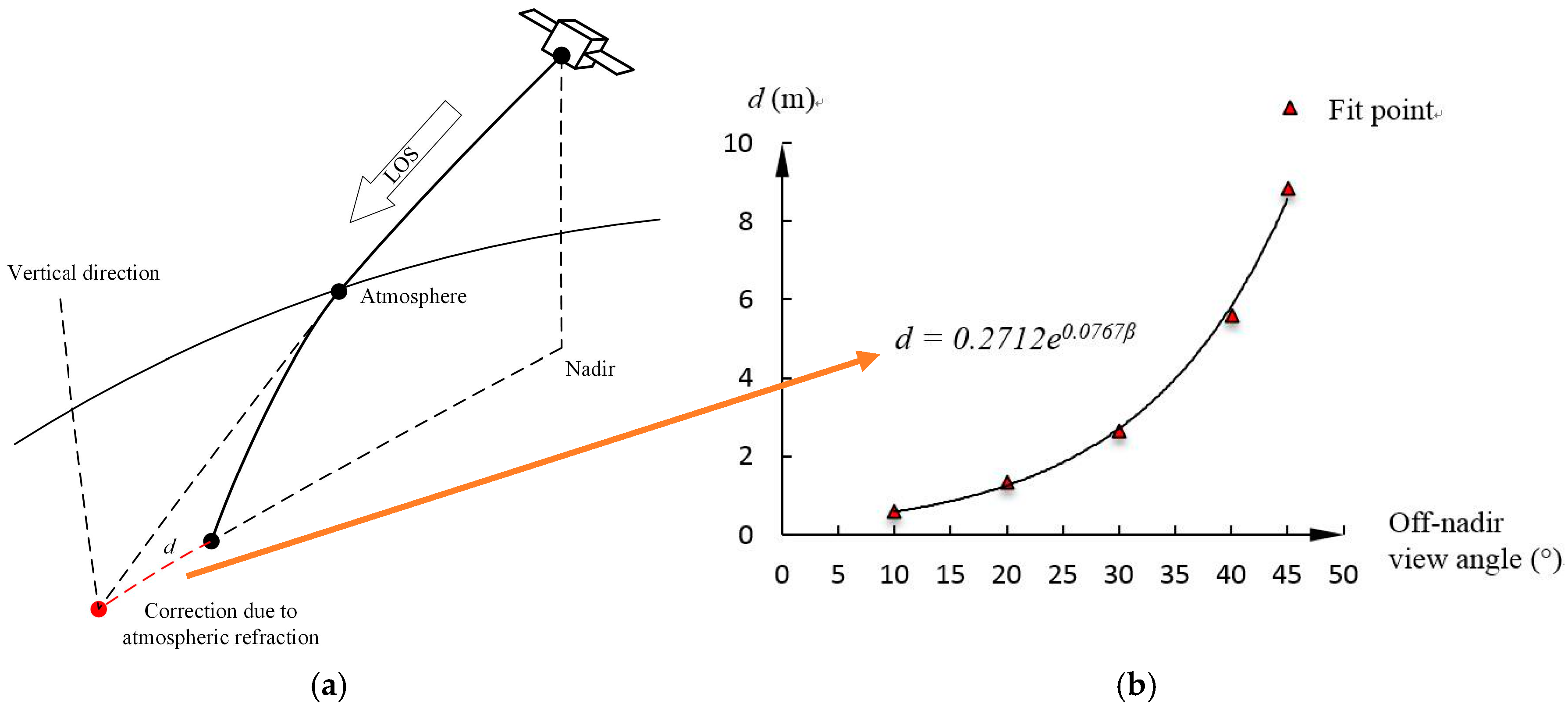
In Earth observation with optical remote sensing satellites, the atmospheric refraction changes the direction of the LOS, resulting in atmospheric refraction geometric deviation. If the off-nadir angle is small, we can ignore the impact of this refraction on the positioning. Currently, optical remote sensing satellite imaging is agile and better able to achieve wide-angle side imaging. In the case of a large side view, we need an accurate model to improve the effect of atmospheric refraction. We can calculate the atmospheric refraction correction of the remote sensing platform from two directions. One is to calculate the change from the satellite to the ground according to the direction of the LOS. The other is to calculate the reflected light from the ground. Figure 7a shows the deviation of the atmospheric refraction from the direction of satellite sight. Many researchers have studied the atmospheric refraction error of remote sensing satellites [29,30,31]. In this paper, we use the calculation method in the literature [32] to calculate the length variation d of the LOS vector after the atmospheric refraction is projected onto the Earth’s surface. To facilitate the later calculation, we use an exponential function to fit the atmospheric refractive error d values at different lateral angles, as shown in Figure 7b.

After the atmospheric refraction is corrected, the coordinates of the ground point can be determined from Equation (23).

$$\overrightarrow{{P″}_E}=\overrightarrow{{P\prime }_E}-d\times \left[\begin{array}{c}\sin (a)\\ \cos (a)\\ 0\end{array}\right]$$

(23)

where α is the mean azimuth of the satellite.

Now, after the velocity aberration correction, the optical path delay correction, and the atmospheric refraction correction, we have created a refined WV02 satellite physical model.

4. RFM Modeling

The rational function model (RFM) uses a rational function to represent the mathematical correspondence between the object point and the image point, which is independent of the sensor’s type and does not require sensor parameters. The calculation of the rational function coefficient requires a certain control point. According to the acquisition method of the control point, the calculation method of the rational function coefficient is divided into two methods: correlation with and without terrain. Generally, we use a method independent of the terrain, that is, we generate a large number of virtual control points to calculate the rational function coefficient. This method can achieve nearly the same precision as the rigorous sensor model [10,11,15,16].

4.1. Basic Principles

The rational function model is defined as the point coordinate’s polynomial ratio of the object space (X,Y,Z) to the image space (r,c). In this model, in addition to the polynomial coefficient, object space and image space point coordinates, and without other parameters, the rational function model of the mathematical expression is as follows:

$$\begin{array}{l}{r}_n=\frac{P_1(X_n,Y_n,Z_n)}{P_2(X_n,Y_n,Z_n)}\\ c_n=\frac{P_3(X_n,Y_n,Z_n)}{P_4(X_n,Y_n,Z_n)}\end{array}\}$$

(24)

In Equation (21), to overcome the rounding error caused by the large data level difference, it is necessary to normalize the coordinates in both the object and image spaces. By translating and scaling, we can regularize the pixel coordinates (r,c) and the object coordinates (X,Y,Z) to the normalized coordinates (r_n,c_n) and (X_n,Y_n,Z_n), whose values are in the range (−1.0, +1.0). The specific form of P_i is as follows:

$$\begin{array}{l}{P}_{i=1,2,3,4}(X,Y,Z)={\displaystyle \sum _{i=0}^3{\displaystyle \sum _{j=0}^3{\displaystyle \sum _{k=0}^3{a}_{ijk}{X}^i{Y}^j{Z}^k}}}=a_0+a_{1}X+a_{2}Y+a_{3}Z+a_{4}XY+a_{5}XZ+a_{6}YZ+a_7{X}^2+a_8{Y}^2\\ +a_9{Z}^2+a_{10}XYZ+a_{11}{X}^{2}Y+a_{12}{X}^{2}Z+a_{13}X{Y}^2+a_{14}{Y}^{2}Z+a_{15}X{Z}^2+a_{16}Y{Z}^2+a_{17}{X}^3+a_{18}{Y}^3+a_{19}{Z}^3\end{array}$$

(25)

where a_ijk are the rational polynomial coefficients (RPCs).

4.2. Physical Reverse Model

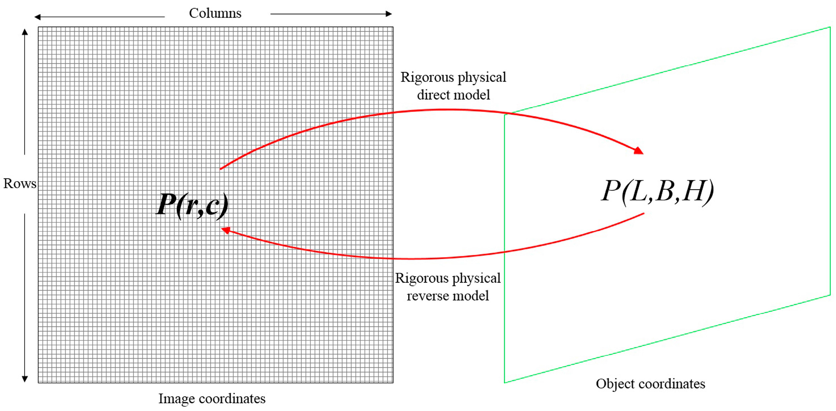
To calculate the RPCs, we must obtain the image coordinates corresponding to the object’s virtual control points. This calculation is achieved by an inverse transform model (Figure 8).

There are two primary methods to realize the inverse transformation: the iterative inverse of the collinear formula model and the direct inverse transformation based on the rational polynomial model. The former is suitable for traditional CCD linear array push-broom images where the integration time is fixed; the high-resolution images of the SPOT5 satellite are typical. This method must calculate the corresponding line scanning time by iteration, and then calculate the coordinates of the corresponding point in the image space. To restore the original image-line relationship, one must also know the level-1B image and the raw image conversion relationship. SPOT images provide a cubic polynomial model for calculating the level-1B image from the original image [26]. This method is computationally complex and inefficient.

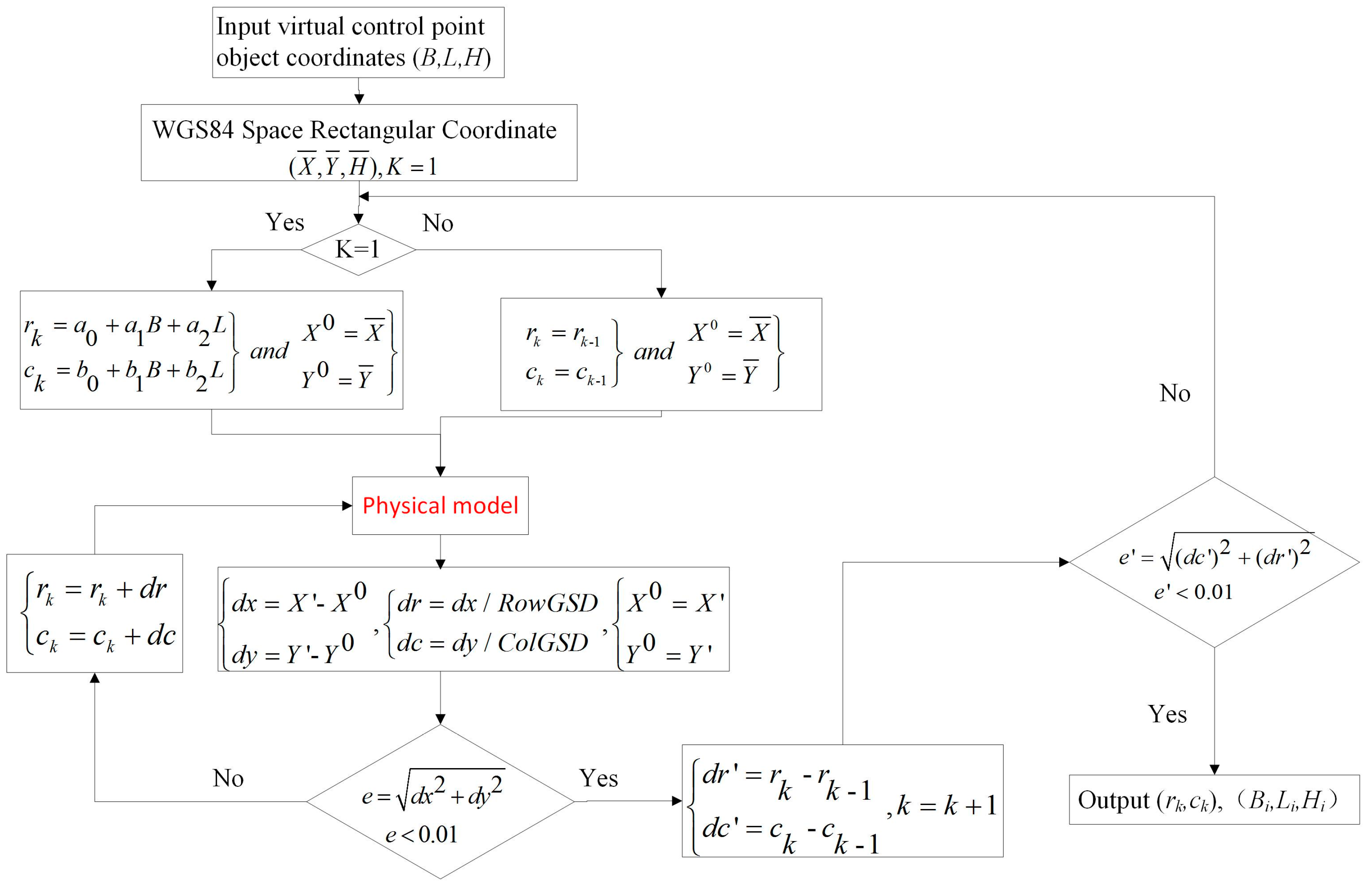
If we know the RPC inverse model coefficients, we can easily calculate the object space to the image space. For WV02 satellite imagery, DG does not provide an inverse model based on RFM, nor does it provide the raw image. Therefore, we cannot use either of these methods. In this paper, we proposed a two-layer iterative method to perform the inverse transformation method of the image coordinates. This method is insensitive to the initial bit value of the iteration, and the calculation method is simple and stable. The algorithm makes full use of the information of the WV02 image support file, and the most significant difference from the existing method is the use of a double iterative structure. The calculation steps for this method are as follows::

• We enter the virtual control point object coordinates and latitude and longitude coordinates, and transform them into WGS84 Cartesian coordinates.
• Based on the coordinates of the image’s four corners, we establish the rough correspondence between the object space and the image space by using the two-dimensional affine transformation method. We use the least squares method to calculate the transformation coefficients. We input the virtual control point object coordinates; then, we find the initial coordinates in the image space by using Equation (26).

  $$\begin{array}{l}r=a_0+a_{1}X+a_{2}Y\\ c=b_0+b_{1}X+b_{2}Y\end{array}\}$$

  (26)
• Based on the initial image coordinates and elevation, we use the physical model to calculate the coordinates in the object space.
• To calculate the difference between the coordinates in the object space, we use the pixel resolution to transform the difference to the image space. To update the image coordinates, we re-enter the physical model. If the result is less than a certain tolerance, we exit the process.
• We update the initial coordinates in the image space and return to Step 4. If the result is less than a certain tolerance, we exit the process.
• We output the point coordinates in the object and image spaces.

The process is shown in Figure 9.

4.3. Calculation of the RPC Coefficients

Currently, the least squares (LS) iterative method is the primary method used to calculate the RPC parameters. Due to the excessive parameterization of the model, which causes inconsistency in the formula matrix, the RPC parameters are unstable and the least squares are not convergent. The result may have some biases from the true value. The ridge estimation method proposed by Hoerl and Kennard in 1970 is considered to be one of the effective ways to solve the ill-conditioned formula [33,34]. Tao and Hu use this method for calculating the RPC coefficients. Their research shows that ridge estimates can achieve well-structured, high-order terms close to zero for the RPC parameters. The disadvantage of the ridge estimation method is because the changing equivalent relation of the formula is changed, the estimation results are biased.

4.3.1. Correcting Characteristic Value Method (CCVM)

Xinzhou et al. [35] proposed a spectral correction iterative method, which is a method that not only maintains the numerical stability in the process of solving the formula but also does not change the equivalent relation of the formula, so the calculation result is not biased. In this paper, we use the least squares and correcting characteristic value methods to calculate the RPC coefficients and compare their results. The solution for the correcting characteristic value method is described below.

The error equation is as follows:

$$(A^{T}PA)X=A^{T}PL$$

(27)

If we add X to both sides of Equation (27), we obtain the following:

$$(A^{T}PA+E)X=A^{T}PL+X$$

(28)

where E is an n-order unit matrix. Since both sides of the equation contain unknown parameter X, they can only be solved by the iterative method. The iterative equation is as follows:

$$x^{(n)}={(A^{T}PA+E)}^{-1}(A^{T}PL+x^{(n-1)})$$

(29)

where $x^{(n)}$ is the nth spectrum of the X correcting characteristic value.

Since the matrix $A^{T}PA$ adds the unit matrix E, it becomes the matrix $(A^{T}PA+E)$, reducing the number of conditions and improving the formula of morbidity. For any initial value $x^{(0)}$, there are the following:

$$\underset{n\to \infty }{\lim }{x}^{(n)}={(A^{T}PA)}^{-1}(A^{T}PL)$$

(30)

Through the above proof, we can determine that the solution is an unbiased estimate.

4.3.2. RPC Coefficient Calculation Flow

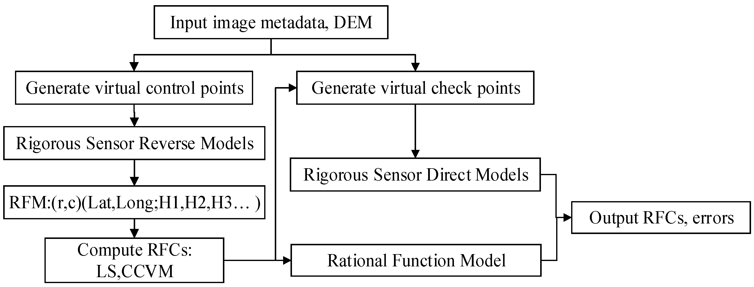
Virtual control point generation selects a plane with a 10 × 10 grid size, stratifies the elevation into 10 layers and doubles the checkpoint plane density. The RPC coefficient calculation process is shown in Figure 10.

5. Results

5.1. Physical Model Experiment

We use the algorithm from Section 3 to experiment with the direct positioning accuracy of the WV02 L1B panchromatic monolithic image in the study area. We use all ground control points in the experimental area as independent checkpoints (ICPs) and use UTM projection to develop the plane coordinate system. We use the root mean square error (RMSE) to represent the positioning errors as follows:

$$\begin{array}{l}RMS{E}_X=\sqrt{\frac{{\displaystyle \sum {(X_{image}-X_{ICP})}^2}}{n}}\\ RMS{E}_Y=\sqrt{\frac{{\displaystyle \sum {(Y_{image}-Y_{ICP})}^2}}{n}}\\ \\ RMS{E}_r=\sqrt{{(RMS{E}_X)}^2+{(RMS{E}_Y)}^2}\end{array}\}$$

(31)

Four images’ direct geometric positioning errors are shown in

Table 2. Horizontal positioning error for single images.

Scene Number	Number of ICPs	Mean Off Nadir View Angle (°)	RMSEX (m)	RMSEY (m)	RMSEr (m)
15JUL10043733-	49	17.8	6.3	1.6	6.5
15JUL10043857-	46	24.5	1.6	1.9	2.5
15JUL24042129-	48	33.1	4.1	3.8	5.6
15JUL24042233-	38	17.6	1.7	1.3	2.2

. We use the stereo triangulation method to calculate the homonymous point coordinates from the cameras to the ground. Two stereo pair’s location errors are shown in

Table 3. Horizontal positioning error of stereo pairs.

Stereo Pair	Scene Number	Mean Off Nadir View Angle (°)	ICPs Num	RMSEX (m)	RMSEY (m)	RMSEr (m)
I	15JUL10043733 + 15JUL10043857	17.8 + 24.5	40	3.4	1.7	3.9
II	15JUL24042233 + 15JUL24042129	17.6 + 33.1	31	1.4	2.2	2.6

.

We calculated the horizontal accuracy with a circular error at 90% confidence (CE90) and a height error with a linear error at 90% probability (LE90) (see Equation (32)) [36] as follows:

$$\begin{array}{l}RMSEc=0.5(RMS{E}_{\min }+RMS{E}_{\max })\\ CE90=2.146·RMSEc\\ LE90=1.644·RMS{E}_H\end{array}\}$$

(32)

Four images and two stereo pairs’ horizontal location errors are shown in Figure 11.

As seen in Figure 11, the CE90 error of the monolithic image direct geometric positioning is 6.7 m, and the stereo pair’s CE90 error is 5.0 m. The ICP’s absolute vertical accuracy of the stereo pair is 3.0 m. This result is consistent with the WV02 nominal accuracy. It can be seen that the physical positioning errors are relatively stable, reflecting the existence of a certain deviation. Primarily due to star tracker cameras and on-board GPS receivers causing positioning errors, this error can almost be eliminated by using a few GCPs.

5.2. Rational Function Model Experiment

We use the RPC method, described in Section 4.3, LM and CCVM to determine the RPC solution. A 10 × 10 virtual control point grid is used, with the elevation divided into 10 layers. We use the calculated RPCs to calculate the image coordinate error of the ICPs. The calculation results for the four images are shown in

Table 4. The rational function model (RFM) errors of the independent checkpoints (ICPs) (meters).

Method	Correcting Characteristic Value Method (CCVM)			Least Squares(LS)			DigitalGlobe (DG)
Scene Number	RMSEX	RMSEY	RMSEr	RMSEX	RMSEY	RMSEr	RMSEX	RMSEY	RMSEr
15JUL10043733-	5.1	1.6	5.3	5.1	1.6	5.4	11.9	5.1	6.7
15JUL10043857-	2.3	1.8	2.9	2.3	1.9	3.0	1.5	2.5	2.9
15JUL24042129-	2.8	3.9	4.8	2.8	4.2	5.0	4.6	1.9	4.9
15JUL24042233-	1.5	1.3	2.0	1.5	1.3	2.0	1.8	2.4	3.0
Mean	2.9	2.2	3.8	2.9	2.3	3.9	5.0	3.0	4.4

. The values in bold indicate the horizontal error of the ICPs, in meters.

As seen in Table 4, the RFM positioning accuracy of the monolithic image is basically identical to the physical model. The positioning accuracy of the CCVM method in three images is nearly identical to the LS, but in one image (15JUL24042129) the CCVM positioning accuracy was significantly better. Specifically, if the design matrix is ill-posed during the calculation process (meaning the matrix contains a larger number of conditions), the LS solution may have a certain deviation and the CCVM solution is unbiased. From the monolithic image RFM location results, the RPC resolution is slightly better than the DG RPC precision in this experiment. The mean error in the monolithic horizontal positioning of the original RPC model is 4.4 m and our method is 3.8 m, which is 13.7% higher than that of the original RPC positioning provided by the imaging company. Additionally, we use the RFM-based stereo intersection method to calculate the positioning error of two stereo pairs (see Figure 12).

As seen in Figure 12, the single image RPC positioning accuracy (CE90) is 6.2 m, superior to the RSM positioning accuracy of 6.7 m. However, the accuracy of the stereoscopic positioning and the RSM are consistent at 5.0 m.

6. Discussion

6.1. The Influence of Elevation on the Accuracy of the Physical Model

The physical model algorithm in this paper must provide a reference DEM based on the DEM of the elevation of iterative interpolation. The accuracy of the elevation value has some effect on the accuracy of the physical model. To describe the effect of elevation error on the plane positioning accuracy, we calculated the change of the projection coordinates caused by a change of 1 m for each elevation under the condition that the image coordinates are unchanged, as shown in

Table 5. Influence of elevation error on plane direct location.

Scene Number	Elevation Change Value (m)	∆x (m)	∆y (m)	∆d (m)
15JUL10043733-	1	0.35	–0.06	0.36
15JUL10043857-	1	–0.46	–0.27	0.53
15JUL24042129-	1	0.58	0.48	0.75
15JUL24042233-	1	–0.05	0.34	0.34

.

In Table 5, it can be seen that each 1 m elevation change due to a horizontal positioning error causes different changes in each image, in the range of 0.3 to 0.8 m. Therefore, we can first calculate the physical model using a rough DEM, then obtain the RPC coefficients, extract the higher-resolution DEM, and recalculate the physical model. This iterative process stops when the elevation value changes less than a specified amount.

6.2. RFM Fit Analysis

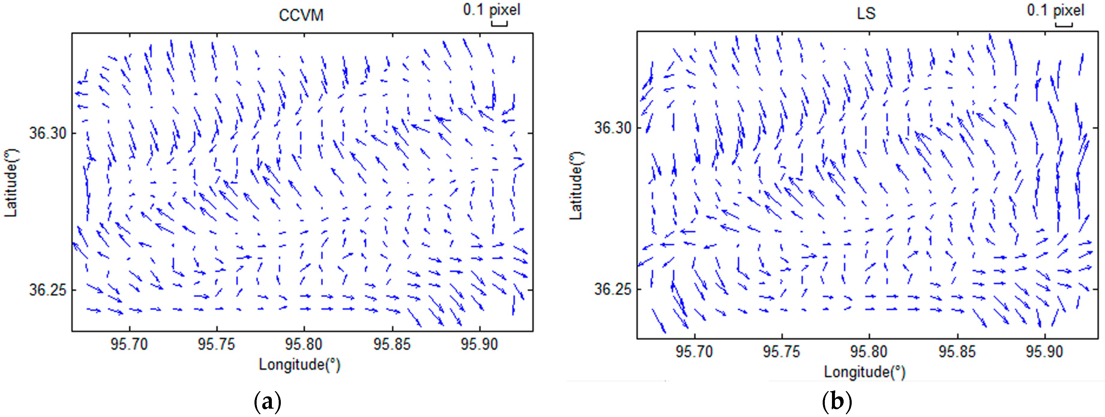
For the precision of RFM fitting the RSM, the conventional idea is to generate the virtual checkpoints and calculate the error between the two models. In this paper, the virtual checkpoint is generated based on the density of 20 × 20 × 10. The accuracy was checked and the results are shown in

Table 6. WV02 single image RFM fit errors (pixels).

RPC Method	CCVM				LS
Scene Number	RMSErow	RMSEcol	MAX Error in Row	MAX Error in Column	RMSErow	RMSEcol	MAX Error in Row	MAX Error in Column
15JUL10043733	0.117	0.104	–0.297	–0.257	0.118	0.104	0.299	0.257
15JUL10043857	0.076	0.142	–0.176	0.336	0.075	0.145	0.175	–0.346
15JUL24042129	0.092	0.069	–0.336	1.276	0.092	0.147	–0.336	6.444
15JUL24042233	0.087	0.168	–0.199	0.446	0.087	0.181	–0.198	0.473

and Figure 13.

In Table 6, it can be seen that in four images the CCVM accuracy is slightly better than the accuracy of LS. In the 15JUL24042129 image (the values in bold), this difference is especially obvious.

While with a virtual control point check the error between the RFM and the RSM is small, it is better to use an actual control point to check the accuracy. This also indicates that the RPC model may generally have better precision when using evenly distributed checkpoints, but with an irregularly distributed control point for inspection, accuracy, or undulation.

In the case of a large number of checkpoints, such as computer stereo matching obtaining the homonymous points, this difference becomes insignificant, and we can consider the physical model and the RFM model accuracy to be almost identical.

7. Conclusions

Based on the characteristics of the WV02 satellite ISD file, this paper elaborates the construction process of the WV02 satellite image geometric orientation using the RSM and RPC models. In the process of constructing the WV02 satellite image using the RSM model, we considered the influence of velocity aberration, optical path delay and atmospheric refraction in the satellite imaging process, and established a new physical inverse model. The inverse model differs from the existing model by two iterations in each of the object and image spaces. Through this inverse model, we can convert point positions of the object space into the image space. In this manner, the virtual control grid is established in the object space to calculate the RPC coefficients. Two methods, CCVM and LS, are used to compare the RPC coefficient calculation process. The CCVM provides basically the same accuracy as the LS, but it is more stable and has superior accuracy. Under the uncontrolled condition, the monolithic horizontal RMSE of the RPC model is 3.8 m. The stereo pairs’ horizontal positioning accuracy of the physical and RPC models are both 5.0 m (with CE90). This paper resolves the RPC accuracy better than the original RPC location accuracy provided by the commercial vendors. Although this work focuses on WorldView-2 data, VHR stereo pairs collected by DigitalGlobe, such as IKONOS, QuickBird-2, and GeoEye-1, can also be analyzed using the methods described in this paper.

References

- Okamoto, A. Orientation theory of ccd line-scanner images. Int. Arch. Photogramm. Remote Sens. 1988, 27, 609–617. [Google Scholar]
- Light, D.L.; Brown, D.; Colvocoresses, A.; Doyle, F.; Davies, M.; Ellasal, A.; Junkins, J.; Manent, J.; McKenney, A.; Undrejka, R. Satellite photogrammetry. Man. Photogramm. 1980, 4, 883–977. [Google Scholar]
- Toutin, T. Review article: Geometric processing of remote sensing images: Models, algorithms and methods. Int. J. Remote Sens. 2004, 25, 1893–1924. [Google Scholar] [CrossRef]
- Giannone, F. A Rigorous Model for High Resolution Satellite Imagery Orientation. Available online: http://citeseerx.ist.psu.edu/viewdoc/download?doi=10.1.1.529.4356&rep=rep1&type=pdf (accessed on 23 June 2017).
- Crespi, M.; Giannone, F.; Poli, D. Analysis of Rigorous Orientation Models for Pushbroom Sensors. Applications with Quickbird. Available online: http://www.isprs.org/proceedings/xxxvi/part1/papers/T02-07.pdf (accessed on 23 June 2017).
- Crespi, M.; Fratarcangeli, F.; Giannone, F.; Pieralice, F. Sisar: A Rigorous Orientation Model for Synchronous and Asynchronous Pushbroom Sensors Imagery. Available online: http://www.isprs.org/proceedings/XXXVI/1-W51/paper/crespi_etal.pdf (accessed on 23 June 2017).
- Crespi, M.; Fratarcangeli, F.; Giannone, F.; Pieralice, F. A new rigorous model for high-resolution satellite imagery orientation: Application to eros a and quickbird. Int. J. Remote Sens. 2012, 33, 2321–2354. [Google Scholar] [CrossRef]
- De Venecia, K.J.; Paderes, F., Jr.; Walker, A.S. Rigorous sensor modeling and triangulation for orbview-3. In Proceedings of the ASPRS Annual Conference, Reno, NV, USA, 1–5 May 2006. [Google Scholar]
- Tao, C.V.; Yong, H. 3d reconstruction methods based on the rational function model. Photogramm. Eng. Remote Sens. 2002, 68, 705–714. [Google Scholar]
- Tao, C.V.; Hu, Y. A comprehensive study of the rational function model for photogrammetric processing. Photogramm. Eng. Remote Sens. 2001, 67, 1347–1358. [Google Scholar]
- Tao, C.V.; Hu, Y. Use of the rational function model for image rectification. Can. J. Remote Sens. 2001, 27, 593–602. [Google Scholar] [CrossRef]
- Cheng, P.; Toutin, T. Ortho rectification and dem generation from high resolution satellite data. In Proceedings of the 22nd Asian Conference on Remote Sensing, Singapore, 5–9 November 2001; p. 9. [Google Scholar]
- Yang, X. Accuracy of rational function approximation in photogrammetry. In Proceedings of the ASPRS Annual Conference, Taipei, Taiwan, 4–8 December 2000; pp. 22–26. [Google Scholar]
- Grodecki, J.; Dial, G. Block adjustment of high-resolution satellite images described by rational polynomials. Photogramm. Eng. Remote Sens. 2003, 69, 59–68. [Google Scholar] [CrossRef]
- Dial, G.; Grodecki, J. Block adjustment with rational polynomial camera models. In Proceedings of the ASPRS 2002 Conference, Washington, DC, USA, 19–26 April 2002; pp. 22–26. [Google Scholar]
- Dial, G.; Grodecki, J. RPC Replacement Camera Models. Available online: http://128.46.154.21/jshan/proceedings/asprs2005/Files/0031.pdf (accessed on 23 June 2017).
- Hu, Y.; Tao, V.; Croitoru, A. Understanding the Rational Function Model: Methods and Applications. Available online: http://www.isprs.org/proceedings/XXXV/congress/comm4/papers/423.pdf (accessed on 23 June 2017).
- Hu, Y.; Tao, C.V. Updating solutions of the rational function model using additional control information. Photogramm. Eng. Remote Sens. 2002, 68, 715–724. [Google Scholar]
- Xuwen, Q.; Shufang, T.; Youtang, H.; Guo, Z. The algorithm for parameters of rpc model without initial value. Remote Sens. Land Resour. 2005, 4, 7–11. [Google Scholar]
- DigitalGlobe. Worldview-2 Spacecraft Information and Specifications. Available online: https://www.digitalglobe.com/resources/satellite-information (accessed on 9 March 2017).
- DigitalGlobe. Accuracy of Worldview Products. Available online: https://dg-cms-uploads-production.s3.amazonaws.com (accessed on 9 March 2017).
- Aguilar, M.A.; del Mar Saldana, M.; Aguilar, F.J. Generation and quality assessment of stereo-extracted dsm from geoeye-1 and worldview-2 imagery. IEEE Trans. Geosci. Remote Sens. 2014, 52, 1259–1271. [Google Scholar] [CrossRef]
- Aguilar, M.A.; del Mar Saldaña, M.; Aguilar, F.J. Assessing geometric accuracy of the orthorectification process from geoeye-1 and worldview-2 panchromatic images. Int. J. Appl. Earth Obs. Geoinf. 2013, 21, 427–435. [Google Scholar] [CrossRef]
- Shean, D.E.; Alexandrov, O.; Moratto, Z.M.; Smith, B.E.; Joughin, I.R.; Porter, C.; Morin, P. An automated, open-source pipeline for mass production of digital elevation models (dems) from very-high-resolution commercial stereo satellite imagery. ISPRS J. Photogramm. Remote Sens. 2016, 116, 101–117. [Google Scholar] [CrossRef]
- Updike, T.; Comp, C. Radiometric Use of Worldview-2 Imagery. Available online: https://dg-cms-uploads-production.s3.amazonaws.com/uploads/document/file/104/Radiometric_Use_of_WorldView-2_Imagery.pdf (accessed on 9 March 2017).
- Riazanoff, S. Spot 123-4-5 Geometry Handbook; Tech Rep. GAEL-P135-DOC-001; GAEL Consultant: Champs-sur-Marne, France, 2004. [Google Scholar]
- Boyd, J.P. Chebyshev and Fourier Spectral Methods, 2nd ed.; Courier Corporation: North Chelmsford, MA, USA, 2001; pp. 19–57. [Google Scholar]
- Barrera, T.; Hast, A.; Bengtsson, E. Incremental spherical linear interpolation. In Proceedings of the Annual Special Theme-Environmental Visualization Conference (SIGRAD), Gold Coast, Australia, 17–22 May 2004; pp. 7–10. [Google Scholar]
- Noerdlinger, P.D. Atmospheric refraction effects in earth remote sensing. ISPRS J. Photogramm. Remote Sens. 1999, 54, 360–373. [Google Scholar] [CrossRef]
- Saastamoinen, J. Contributions to the theory of atmospheric refraction. Bull. Géod. (1946–1975) 1973, 107, 13–34. [Google Scholar] [CrossRef]
- Saastamoinen, J. Introduction to practical computation of astronomical refraction. Bull. Géod. (1946–1975) 1972, 106, 383–397. [Google Scholar] [CrossRef]
- Ming, Y.; Zhiyong, W.; Chengy, W.; Bingyang, Y. Atmosphere refraction effectsin object locating for optical satellite remote sensing images. Acta Geod. Cartogr. Sin. 2015, 44, 995–1002. [Google Scholar]
- Hoerl, A.E.; Kennard, R.W. Ridge regression: Biased estimation for nonorthogonal problems. Technometrics 1970, 12, 55–67. [Google Scholar] [CrossRef]
- Hoerl, A.E.; Kennard, R.W. Ridge regression: Applications to nonorthogonal problems. Technometrics 1970, 12, 69–82. [Google Scholar] [CrossRef]
- Xinzhou, W.; Dingyou, L.; Qianyong, Z.; Hailan, H. The iterration by correcting characteristic value and its application in surveying data processing. J. Heilongjiang Inst. Technol. 2001, 15, 3–6. [Google Scholar]
- Greenwalt, C.R.; Shultz, M.E. Principles of Error Theory and Cartographic Applications; Aeronautical Chart And Information Center: St. Louis, MO, USA, 1962.
Figure 1.
Raw and level-1B image sensor geometry: (a) raw image; and (b) using a virtual scan line to generate the level-1B image with smooth ephemeris and attitude.
Figure 2.
Study area location and stereo pair composition (gray indicates the study area).
Figure 3.
Ground control points (GCPs) distribution in the test area.
Figure 4.
Spatial coordinate conversion process.
Figure 5.
Physical sensor model geolocation: (a) the positioning principle with a single image; and (b) the physical sensor model direct location process.