High Precision DEM Generation Algorithm Based on InSAR Multi-Look Iteration


1
School of Resource and Environmental Sciences, Wuhan University, No. 129, Luoyu Rd., Wuhan 430079, China
2
Satellite Surveying and Mapping Application Center, National Administration of Surveying, Mapping and Geo-Information, Haidian Dist., Beijing 100048, China
3
Jiangsu Center for Collaborative Innovation in Geographical Information Resource Development and Application, Nanjing 210046, China
4
Faculty of Geosciences and Environmental Engineering, Southwest Jiaotong University
*
Author to whom correspondence should be addressed.
Remote Sens. 2017, 9(7), 741; https://0-doi-org.brum.beds.ac.uk/10.3390/rs9070741
Submission received: 13 April 2017
/
Revised: 8 July 2017
/
Accepted: 16 July 2017
/
Published: 18 July 2017
(This article belongs to the Section Remote Sensing in Geology, Geomorphology and Hydrology)
Abstract
:Interferometric Synthetic Aperture Radar (InSAR) is one of the most sufficient technologies to provide global digital elevation modeling (DEM). It unwraps the interferometric phase to provide observations for phase-to-height conversion. However, the phase gradient has great influence on the phase unwrapping quality, thereby affecting the topographic mapping accuracy. Multi-look processing can improve the reliability of phase unwrapping by reducing the noise phase gradient. Nevertheless, it reduces the spatial resolution while increasing the height phase gradient, thus lowering the reliability of height values. In this paper, we propose a multi-look iteration algorithm to suppress the noise and maintain the reliability of height values. First, we use a large number of looks (NL) to suppress the noise phase gradient and obtain a coarse DEM. Then taking this coarse DEM as a reference, we remove the topographic phase from the interferogram with a small NL, which will reduce height phase gradient and ensure the accuracy of phase unwrapping. Finally, we obtain DEM products with high precision and fine resolution. We validate the proposed algorithm using both simulated and real data, and obtain DEM products in a greatly undulated region using TanDEM-X data. Results show that the proposed method is capable of providing DEM with resolution of 4 m and accuracy of 1.73 m.
1. Introduction
The digital elevation model (DEM) with both high spatial resolution and height accuracy is widely used in scientific applications [1]. For instance, DEM is able to provide reference for urban infrastructure deformation monitoring [2,3], coseismic deformation extraction of earthquakes [4,5,6], as well as landslide monitoring [7,8]. However, it is not easy to produce DEM using optical stereoscopy such as SPOT 5 at global scale [1]. InSAR is one of the most efficient ways to provide global DEMs [9,10,11] due to its all-weather, all-day characteristics, and the automatic high-efficiency processing methods. One of its most successful applications is the shuttle radar topography mission (SRTM). SRTM uses a fixed interferometric baseline to observe the earth’s surface covering 56°S to 60°N [12]. Another success is TanDEM-X. It is able to provide global DEMs including the Antarctica Plate [13]. The 90% point-to-point accuracy of TanDEM-X DEM is declared to be 3.5 m all over the world, 1.3 m if the Antarctica Plate is not considered [13]. Several methods are proposed to ensure the accuracy of the TanDEM-X DEM [14]. First, the parameters of the TanDEM-X system are calibrated using the ground control points [15]. Then, a raw DEM is produced using the calibrated parameters. The Ice, Cloud, and Elevation Satellite (ICESat) data are chosen to calibrate the height ramp error [16]. After that, the descending and ascending data are merged to reduce the layover and shadow areas. Meanwhile, small baseline interferograms are introduced to assist phase unwrapping of long baseline interferograms, aiming at calculating the phase ambiguities correctly [17]. Finally, the tiled DEM data are mosaicked and the systematic errors induced by baseline residues are eliminated [18]. However, the interferometric phase error which affects the DEM quality significantly is only paid close attention to during the satellite system designing stage, but not during the data processing stage [14,19]. Among the interferometric phase error, phase unwrapping is one of the most important errors related to data processing [20,21].
Phase unwrapping is used to integrate the phase gradients (i.e., the phase increment between adjacent pixels). When the phase gradient is great enough (0.822 cycles/pixel for ERS), the spectrum overlap in the range direction disappears, inducing complete decorrelation [20,22,23]. In that case, phase unwrapping cannot obtain any reliable information. Phase gradients are composed of a variety of factors, including phase noise, topographic phase, and other errors (such as baseline error, slant range error). Phase noise is useless and should be eliminated, but the topographic phase is useful and should be retained. As the phase gradients due to the baseline and slant range can be removed through ground calibration [24], it is not covered in this paper.
Decorrelation sources, including signal-to-noise-ratio (SNR) decorrelation, quantization decorrelation, decorrelation of ambiguities, registration decorrelation, spatial decorrelation, temporal decorrelation [14,19], and so on, have complex effects on phase gradients. These decorrelation factors multiply each other and show as randomly distributed noise in the interferogram [25]. The noise has irreversible effects on interferometric phase [20], which means that once the phase decorrelates completely, no useful information can be extracted by data processing. If the interferogram is coherent, i.e., coherence is greater than 0.6, we are able to conduct phase unwrapping [14]. In this case, multi-look processing is able to improve the original coherence by averaging the complex values of a window. The stochastic model between noise phase and number of looks (NL) is discussed by several authors [26,27,28]. Similar models describing the probability density functions (PDF) of interferometric noise phase are also researched [20]. However, the PDF of the noise phase gradient is barely provided. We use the cross-correlation function of the interferometric noise phase PDF to describe the distribution of the noise phase gradient. The characteristics of the PDFs with respect to NLs are investigated in the paper.
The elevation has a linear relationship with the phase gradient. In other words, large terrain undulation brings great phase gradient and low confidence of phase unwrapping [29]. Therefore, in InSAR data processing, we often introduce external DEM data to reduce the terrain undulation [17]. Multi-look processing plays an important role in DEM calculation. Small NLs are preferred to reduce the noise and ensure the pixel spacing of the DEM [30]. Large NLs are also applicable if the interferometric phase is contaminated seriously by noise [31]. However, most of the discussions concentrate on the de-noising capacity of NLs, regarding its effect on elevation phase distortion. Fractional Brownian motion (fBm) is one of the most effective models to describe the DEM’s character because the model is self-similar and long-range dependent [32]. The research of the PDF of elevation phase gradient with respect to NLs is discussed based on fBm.
There is contradiction between the effects of NLs on both the noise phase gradient and elevation phase gradient. We have to adopt large NLs to suppress the noise and small NLs to ensure elevation phase consistency. One solution is to use tomographic SAR (TomoSAR) to solve this contradiction by providing super-resolution DEM data. TomoSAR uses the coherence to model the interferometric complex data, aiming at separating different scatterers within a single pixel [33]. This is more useful than InSAR in the layover regions, especially in the areas covered by high to tall buildings. Meanwhile, the accuracy of TomoSAR is higher given that the different height values of different scatterers are distinguished during modeling. However, TomoSAR is not necessary given two reasons. First, 90% of land covers are distributed scatterers [34] and the layover phenomenon does not appear in those regions. If we use TomoSAR to calculate DEM all over the image scene, that would be a waste of calculating resources. Secondly, ultra-precision elevation values of the buildings are not necessary for DEM extraction. Even if the corresponding data are obtained, we have to edit the information to ensure that the elevations of land covers are eliminated and only the elevations to the ground are maintained. The second solution is to use multi-temporal InSAR (MTInSAR) to obtain DEM data with accuracy of better than a decimeter. MTInSAR is a generic term used in InSAR analysis. For example, Tomo-Diff [34,35], PSI [2], SBAS [36], SqueeSAR [37] are all MTInSAR that use multi-temporal and multi-baseline interferograms. MTInSAR models deformation values, height values, as well as the noise component simultaneously, therefore we have to adopt different perpendicular baselines for different applications’ purposes. Deformation needs a small baseline to eliminate height error, while DEM needs broad baseline coverage to ensure that the elevation error is precisely calculated. MTInSAR technologies are elaborate to calculate pointwise information for the persistent scatterers. However, we have to calculate DEM all over the interferogram, which is not easy for MTInSAR, especially in natural terrain or when the number of the images is limited. Therefore, we prefer to improve the InSAR method instead of the MTInSAR method. Even if MTInSAR were able to provide the precise elevation values of the distributed scatterers, meaning that 90% of the pixels could be calculated, the cost of the SAR images would be inestimable when it is applied in global DEM extraction. That is even more difficult to implement in China because we do not have a domestic, applicable interferometric SAR satellite at present.
In this paper, we propose a multi-look iteration algorithm to provide both high accuracy and fine grid size of the DEM. First, we generate a coarse DEM (CDEM) using the 8 × 8 NL. Although the height phase gradient of CDEM is large, the small noise phase gradient lowers the total phase gradient, ensuring the accuracy of CDEM. However, CDEM has low spatial resolution because of the large NL, so it cannot provide fine DEM data. Taking CDEM as a reference, we can obtain an intermediate DEM (IDEM) using the 4 × 4 NL. In a similar way, we can finally get the DEM data by the 2 × 2 NL. The algorithm is analyzed and validated by both simulated data and TanDEM-X data.
The paper is organized as follows. The second section briefs the relationship among the multi-look algorithm, the noise phase gradient, and the elevation phase gradient. The third section introduces the multi-look iteration algorithm, which is validated by simulated and real data in the fourth section. In section five, we discuss the flexibility of using alternative NLs in the proposed method and the difficulties of geocoding with small NLs. The feasibility of providing DEM with both high-precision and fine grid size is also discussed here. Finally, the conclusion is drawn in the sixth section.
2. Multi-Look Algorithm and Phase Gradient
2.1. Maximum and Minimum Detectable Phase Gradient
The phase gradient is often decomposed into components in azimuth and range directions. Phase unwrapping is to integrate the phase gradients in these two directions. For the interferogram, the integral process can be expressed in a discrete way [38]:
where ϕ is the unwrapped phase, is the phase gradient between two adjacent points (i, j) in the integral path, ∑ is the total value of the data series. The most important step of phase unwrapping is to determine the integral path, in which the objective function should be the minimum [38] as
where is the objective function which represents norm () of phase difference before and after unwrapping, r is the range direction, a is the azimuth direction, is used to ensure that the value of objective function is minimum. Phase gradients affect the phase unwrapping accuracy [23,32,39], but the functional relationship between them is difficult to quantitatively express. In order to study this relationship, Ireneusz Baran et al. proposed a mathematical simulation method to obtain the relationship between the detectable deformation gradient and coherence using Envisat-ASAR [40]. Considering the ASAR wavelength λ (5.6 cm), we can convert the deformation gradient model into the phase gradient model using
where is the deformation gradient, λ is the wavelength. The formula after conversion can be written as:
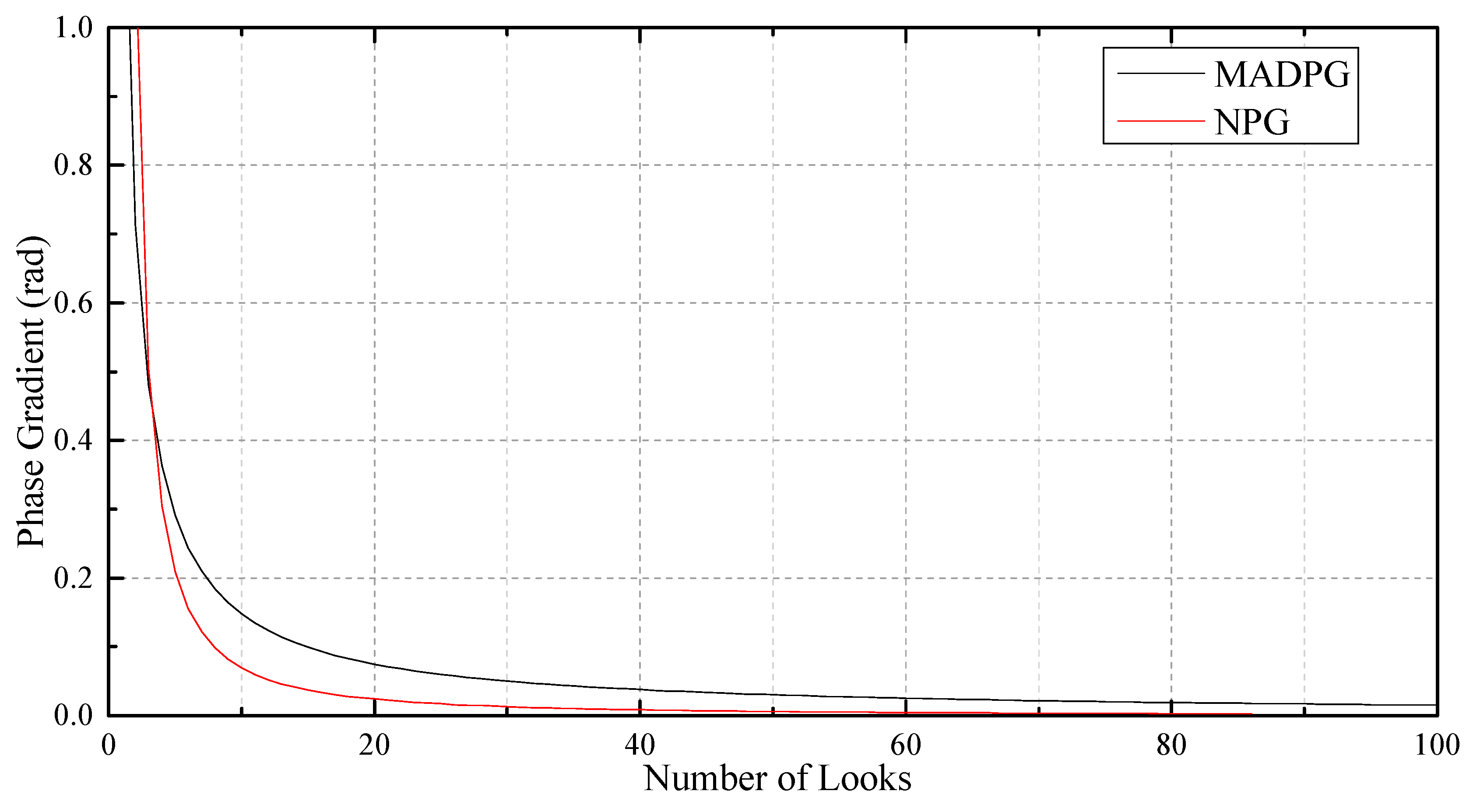
where is the minimum detectable phase gradient(MIDPG), is the maximum detectable phase gradient (MADPG), , and is the azimuth pixel spacing after multi-look processing, is ground pixel spacing after multi-look processing, γ is the coherence. With the coherence 1.0, the minimum detectable phase gradient , the MADPG reaching to its extreme π, almost all the phase changes can be accurately detected. When the coherence decreases, the MIDPG increases and the MADPG reduce. We take the NL as the basis to do phase unwrapping if the MIDPG and MADPG are equal. Taking the stripmap mode of TanDEM-X as an example, with the azimuth pixel spacing 2 m and the NLs 1, 4, and 16, the corresponding minimum coherence coefficients are about 0.55, 0.39, and 0.26, respectively. If the NL is greater than 66, the minimum phase gradient is below 0, which means that any phase less than can be detected. In that case, NLs in both azimuth and range directions are about 8, so 8 × 8 is the largest NL used in this study.
The interferometric phase gradient has similar components to the phase measurement, which can be expressed as
where the five items on the right side are the phase gradient of the flat earth , terrain , deformation , atmospheric delay , and noise, respectively. After accurately removing the flat earth phase, deformation information, and the atmospheric delay, we get a simple equation of the phase gradient as:
For those interferometers with temporal baseline 0 (e.g., SRTM and TanDEM-X), Equation (6) is always the truth, so the phase gradient is determined by the elevation phase gradient (EPG) and noise phase gradient (NPG). EPG is used to calculate the DEM data and should be maintained. While NPG should be removed as well as possible. The MADPG is fixed when the NL is provided, so less EPG allows more NPG, and phase unwrapping can be conducted correctly even with low SNR. Less NPG allows more EPG, meaning that InSAR is more applicable in the surveying and mapping of undulated regions. In the following section, we discuss EPG and NPG from the view of the multi-look algorithm.
2.2. Multi-Look Algorithm
The multi-look algorithm can be employed in two ways in SAR processing. One is to divide the Doppler spectrum into several subsets (number of looks) in the process of image focusing, and sum the independent looks [41]. The other is to average the pixels using a specified window in interferometric processing [20]. In this paper, the multi-look algorithm refers to the latter,
where N is the NL, i.e., the product of the azimuth NL(Na) and the range NL(Nr); is the interferometric pixel values after multi-look processing. and are pixels of the master and slave images before multi-look processing, respectively. is the conjugate of the slave image pixels. a and are the amplitude and phase after multi-look processing, respectively. . is:
where and are real and imaginary parts of a complex number.
2.2.1. Multi-Look Algorithm and Elevation Phase Gradient
Topography has a strong correlation on large scales, while it has stochastic characteristics on small scales, this could be well described by the fractional Brownian motion (fBm) [32]. Assuming that the elevation difference between two adjacent pixels in the azimuth direction is and that in the range direction is , their probability density functions (PDF) using fBm can be expressed as
where
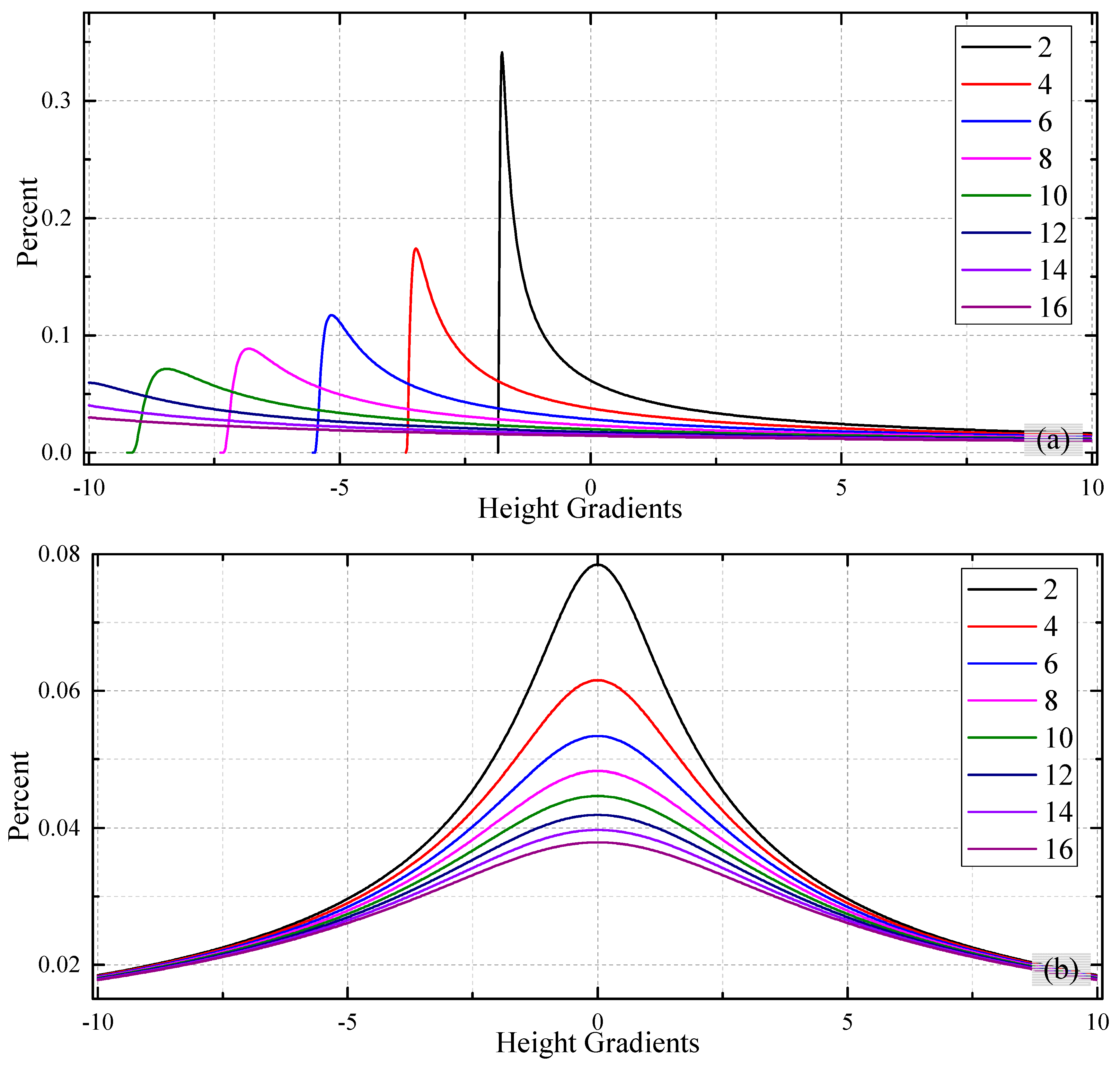
where is the incident angle, and are normalizing constants that can ensure the integral of PDF in its definition domain is 1. H is the Hurst parameter, . H indicates the terrain undulation. If H is close enough to 0, the terrain is totally flat. If H is close to 1, the terrain elevation follows the Gauss stochastic distribution. The experiential value is 0.2 [42]. When , and , we calculate the PDFs in different NLs and show them in Figure 1. Clearly, the distribution of range direction is different from that of azimuth. In fact, the PDF in range direction follows the skewed fBm law because of side-looking geometry. With the increase of the NLs, pixel spacing in the range and azimuth directions grows gradually and the elevation gradient distribution becomes more even, which means the larger the NLs, the more discrete the distribution of the elevation gradient. Therefore, in order to maintain the reliability of elevation, multi-look processing should adopt small NLs which can mostly keep the consistency between the elevation phases in the range and azimuth directions, thereby reducing the elevation phase gradient, and guaranteeing good phase unwrapping results when the noise phase error is high (see Equation (6)).
2.2.2. Multi-Look Algorithm and Noise Phase Gradient
With a NL greater than 1, the PDF of the interferometric phase noise can be expressed as [20]
With a NL equal to 1, the corresponding function is
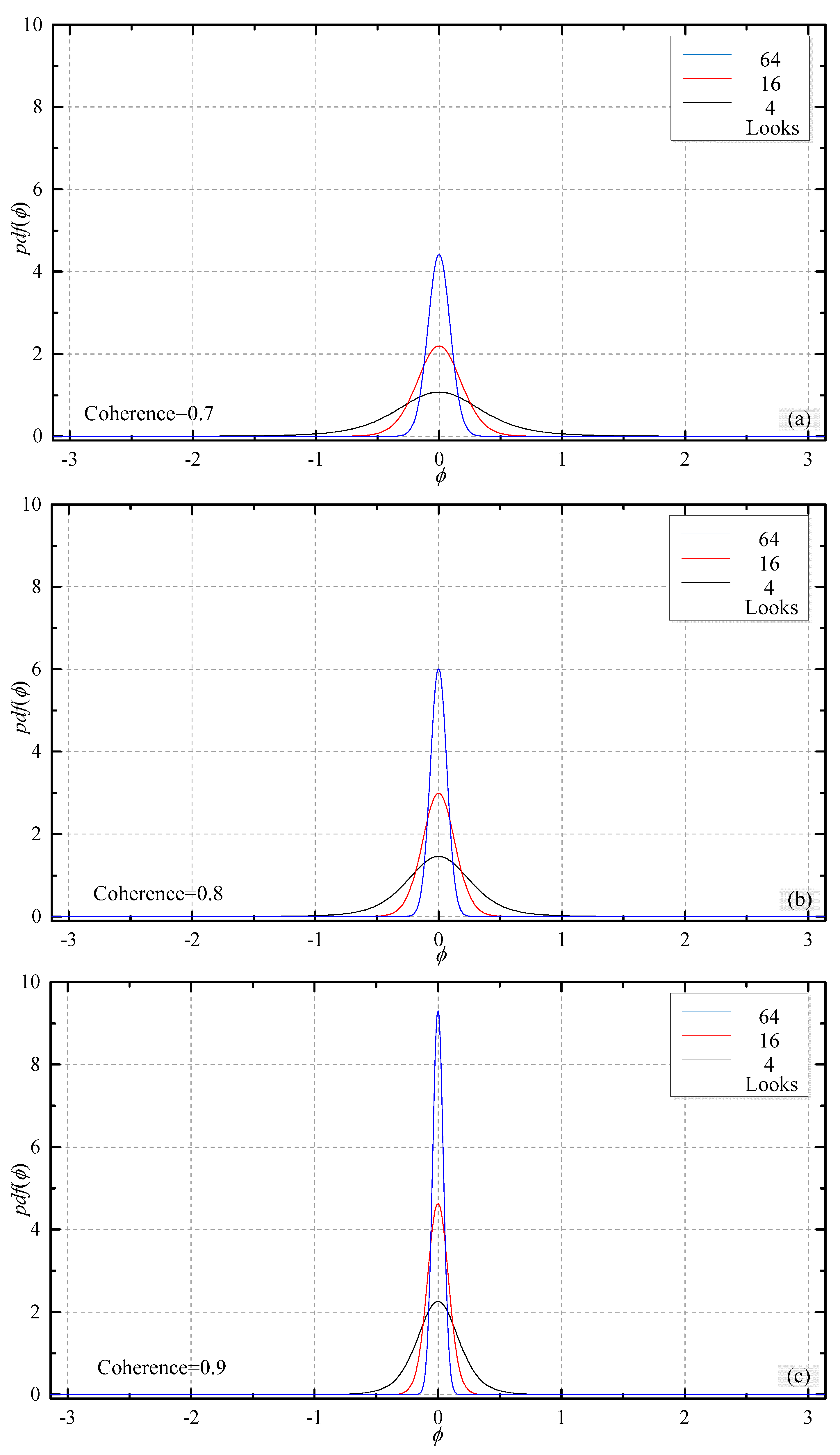
where , is the GAMMA function, N is the NL. Figure 2 shows the PDF of the phase noise with different NLs and coherence. With the same coherence, the larger the NL, the smaller the dispersion of interferometric phase noise, and vice versa. With the same NL, the larger the coherence, the smaller the dispersion of interferometric phase noise, and vice versa. Statistics show that when the mathematical expectation of the phase noise is 0 and coherence is 0.9, NLs of 4, 16, and 64 show corresponding standard deviations 0.206, 0.089, and 0.043 rad, respectively. And with NL 64, the coherence coefficients are 0.7, 0.8, and 0.9, and the interferometric phase standard deviation are 0.091, 0.067, and 0.043 rad, respectively. Therefore, we should choose a larger NL and a higher coherence coefficient to reduce the effect of phase noise.
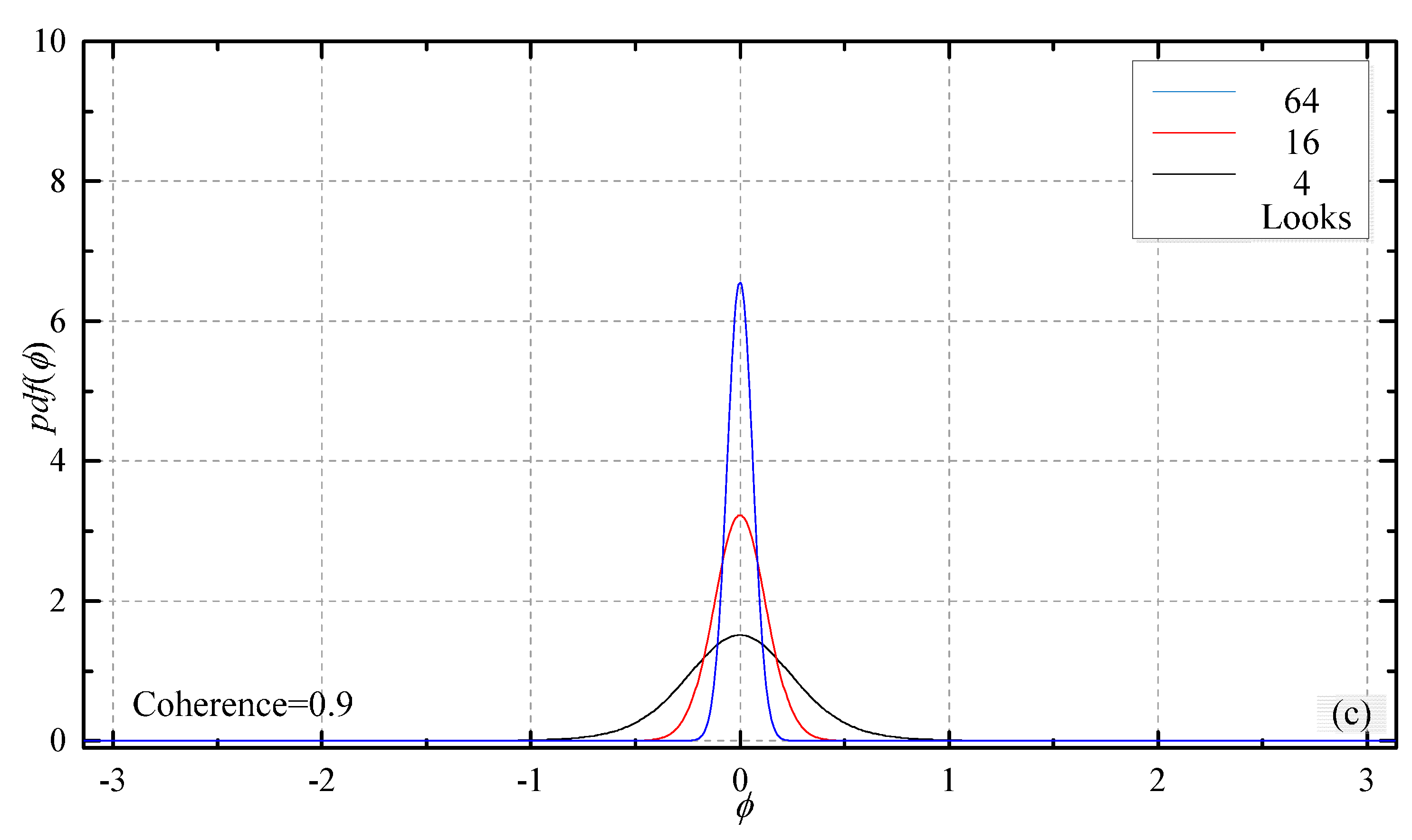
Assuming that the noise of points A and B follows the Gauss hypergeometric distribution, and the two points are independent, the phase gradient of the noise is the cross-correlation function of the noise of the two points [34]. Then the PDF of NPG can be expressed as
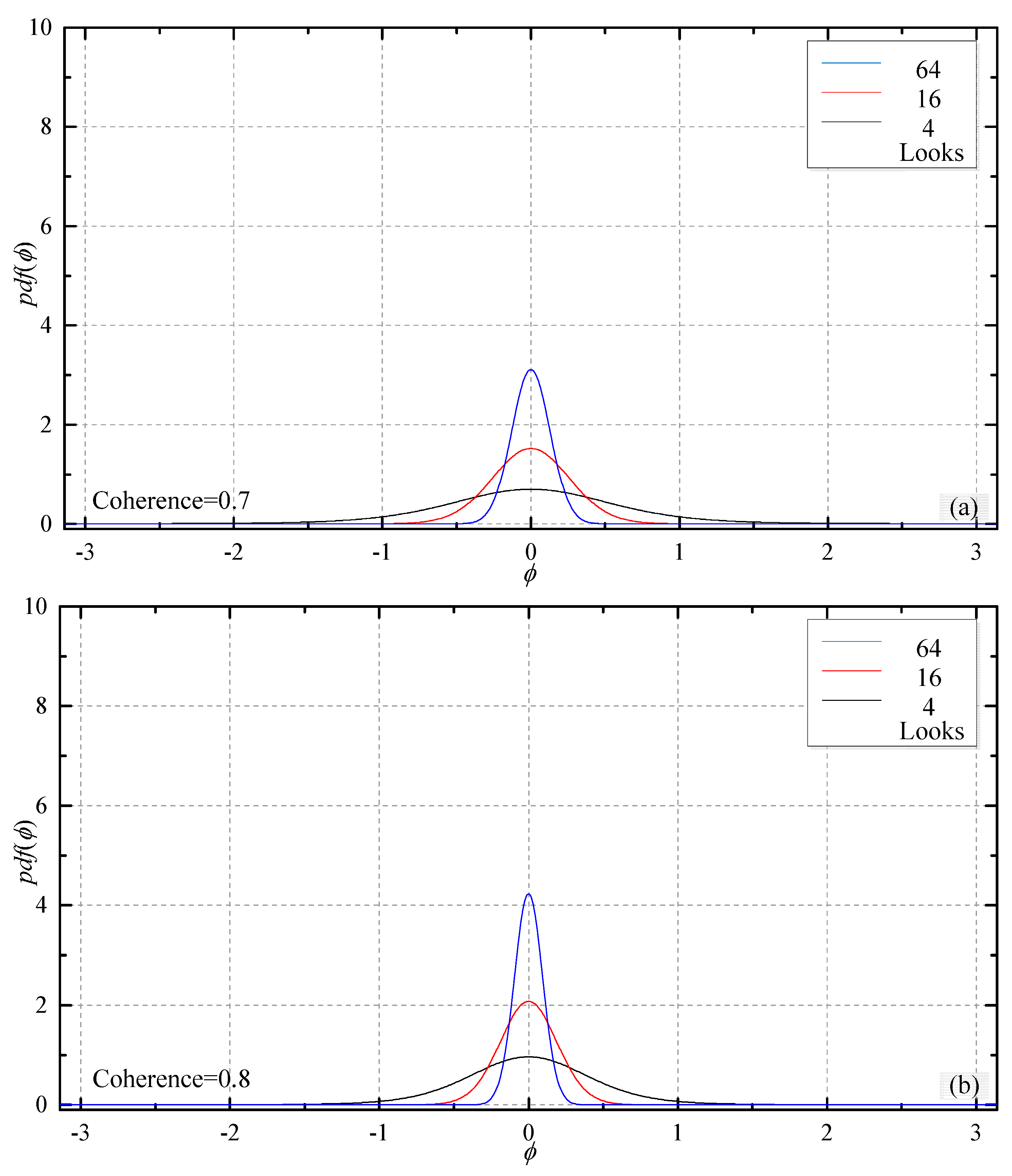
where is the phase wrapping operator, and . Figure 3 shows the distribution of the PDF of the corresponding phase gradient. With the same coherence and NL, the phase gradient PDF in Figure 3 is wider than that in Figure 2, which means the standard deviation of phase gradient is larger than that of phase. Statistical results show that the standard deviation of phase gradient is times the phase standard deviation under the same conditions, which is consistent with the law of error propagation. When other parameters are fixed, a large NL makes the phase gradient approach 0. This allows Equation (6) to contain more EPGs and ensures the reliability of phase unwrapping results in complex terrain.
3. Multi-Look Iteration Algorithm
We propose a multi-look iteration algorithm to reduce the influence of NL on EPG and NPG. The algorithm uses DEMs with larger NLs as reference to calculate finer DEMs with smaller NLs. The CDEM obtained by the NL 8 × 8 processing can only provide basic relief information and can hardly detect any details. Then, the cubic convolution method is used to oversample the CDEM in both the azimuth and range directions. The oversampled elevation value can be taken as the reference to calculate and reduce the terrain phase for the 4 × 4 multi-look processing. Even if the NPG increases, the total phase gradient will not exceed that of 8 × 8, and the accuracy of phase unwrapping as well as IDEM will increase. In the same way, the IDEM can be regarded as the reference terrain for smaller NL processing. When the NL is 2 × 2, the generated DEM can be taken as the final DEM. Because the MADPG is less than the NPG when the NL is smaller than 4 (see Figure 4), reliable phase unwrapping solutions can’t be obtained even in the flat terrain.
4. Experiments
4.1. Validation with Simulated Data
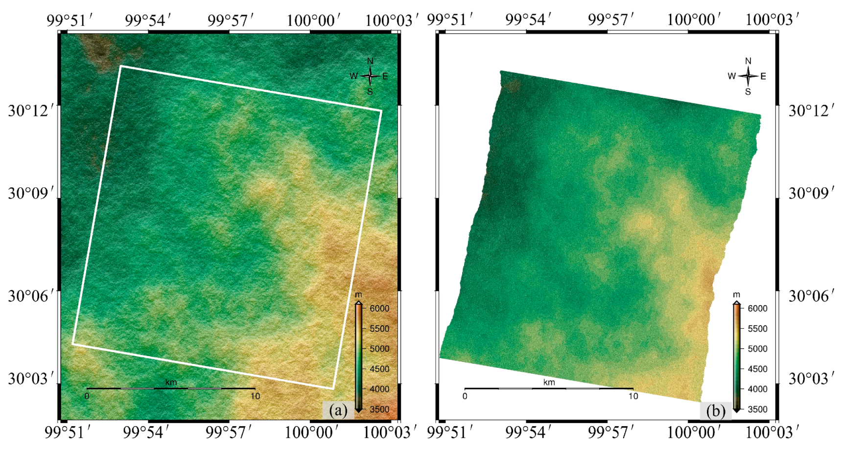
We use the simulated data to validate the algorithm. TanDEM-X data of Litang County in the Ganzi Tibetan Autonomous Prefecture of Sichuan Province are selected. The imaging date is 12 September 2013, and the azimuth and range pixel spacing is 2.19 m and 1.36 m. The looking angle is 42.8 degrees, therefore the corresponding ground pixel spacing is 2 m. The vertical baseline length is 243.7 m, and the near slant range is 657,674.39 m. We crop the single look complex (SLC) image (8000 × 8000) from the original image. With H = 0.7 and 1, we generate a DEM with the size of 8000 × 8000 using the fBm model [42]. As the elevation ranges from 3500 to 6100 m in the study area, we stretch the data and show the results in Figure 5a. The corresponding SLC coverage is shown in Figure 5b.
Assuming the coherence of NL 2 × 2 is 0.9, the interferometric phase standard deviation is 0.206 rad, calculated by the Cramer-Rao formula [20]. As the phases of two SLC images are independent and identically distributed, the phase standard deviation of the single image is 0.146 rad according to Equation (15). We can use Equation (13) to simulate the phase noise of the corresponding master and slave images. We simulate their amplitudes according to the imaging geometry of TanDEM-X and the DEM information. We assume that the slave image only contains the noise information, corresponding to which the SLC can be simulated. Then, we calculate the complex values based on the sum of the flat and terrain phases obtained by interferometric geometric information and the noise phase to form the master SLC.
DEM is then calculated by the traditional method using the simulated master and slave SLCs. This is reverse to the simulation procedures. First of all, we calculate interferograms, remove flat phase, filter, and unwrap the phase. Then we calculate the phase unwrapping constant based on the topographic phase unwrapping results and the simulated topographic phase. Finally, we convert the unwrapped phase to height using the interferometric geometry, and then geocode to obtain the DEM data. The height error of the result is reported as 4.04 m by comparing the simulated DEM and the calculated DEM. Because the solution does not introduce any other errors, the fundamental error is the phase error of the master and slave images, and the derivative error is the phase unwrapping error propagating into the subsequent phase-to-height conversion and geocoding.
The NL influence on the mean absolute value of the EPG (), the NPG () and the total phase gradient () is shown in Figure 6. We calculate with NLs using the simulated data whose noise levels are set to zero. Then we adopt different NLs to calculate by setting the height as a fixed value 3500 m and considering the phase standard deviation 0.146 rad on single SLC. The results show that NPG decreases with the increase of the NLs obviously, especially when the NL is less than 4 × 4. The subsequent increase in the NL does not reduce the phase noise obviously. When the NL is 8 × 8, the NPG is 2.86 degrees and the phase unwrapping error reaches 1.51 degrees which has negligible effect on the elevation. is calculated from the flattened interferogram with only the terrain and noise information. Obviously, if the NL is not bigger than 2 × 2, the total phase gradient decreases with the increase of the NL. This means the main function of multi-looking is to suppress noise if NL is not bigger than 4. If NL is greater than 2 × 2, the terrain information will become dominant in the interferogram, and the total phase gradient has a similar variation trend with the EPG.
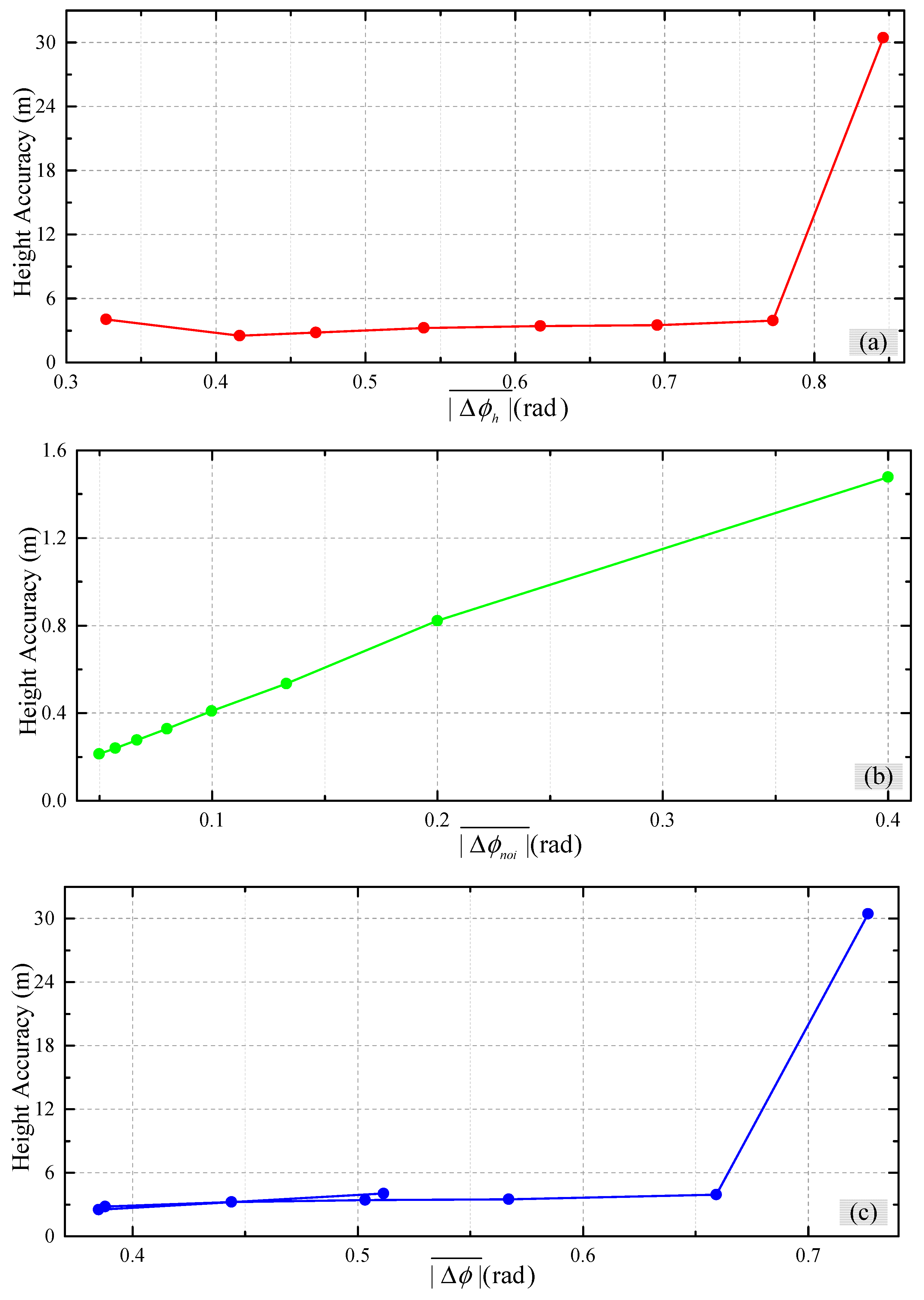
Figure 7 shows the influence of , , and on the height accuracy. When the NL is 1, the influence of the EPG and the total phase gradient on the elevation accuracy has no regulation because of the noise. When NL is bigger than 2 × 2, a large phase gradient lowers elevation accuracy. If NL is greater than or equal to 8 × 8, there will be obvious phase unwrapping error and the elevation accuracy jumps. And the NPG has a strong negative correlation with the elevation accuracy. So in flat areas which are dominated by the NPG, large NLs are preferred to ensure the elevation accuracy.
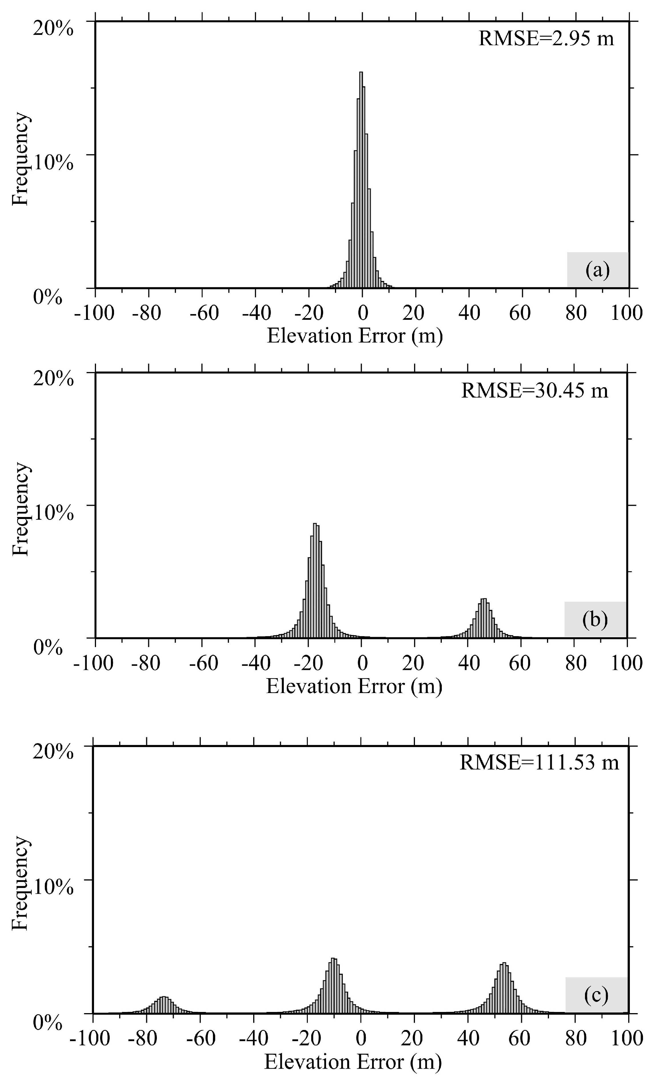
In order to assess the multi-look iteration algorithm, we conduct an experiment with the height ranges from 3500 to 5500 m. The DEM accuracy is 2.95 m after the 8 × 8 multi-look processing (Figure 8a). When it is used as a reference, the accuracy of the IDEM obtained by the 4 × 4 multi-look processing is 2.17 m, but the accuracy of the DEM obtained without iteration is 2.45 m. After the second iteration, the accuracy of DEM after 2 × 2 multi-look processing is 2.10 m, and that without iteration is 2.33 m. Results show that DEM accuracy increases with a decrease in NL. What is more, the multi-look iteration algorithm is able to provide a DEM with higher accuracy than the traditional way if the NL is specified.
8 × 8 NL leads to large phase distortions when the height range increases. This induces phase unwrapping error, thus contaminating the quality of DEMs. For example, if the simulated elevation range is [3500, 6100], the accuracy of DEM obtained by the 8 × 8 multi-look processing is 30.45 m (Figure 8b). In order to ensure the availability of the multi-look iteration algorithm with large elevation difference, we need to introduce external DEM data to reduce the height gradient. External DEM data could be coarse, as long as it can reflect the general elevation difference. We further increase the height difference to [3500, 6500], and take the simulated DEM with 45 times down-sampling as the reference. Results show that the height accuracy surges from 111.53 m (no reference DEM, 8 × 8 NL, Figure 8c) to 8.99 m (8 × 8 NL), and the multi-look iteration method further enhances the accuracy to 3.96 m (4 × 4 NL) and 3.48 m (2 × 2 NL), respectively. Therefore, using the external DEM as a reference can improve the reliability of the phase unwrapping results, and improve the final accuracy of the multi-look iteration algorithm.
4.2. Validation with Real Data
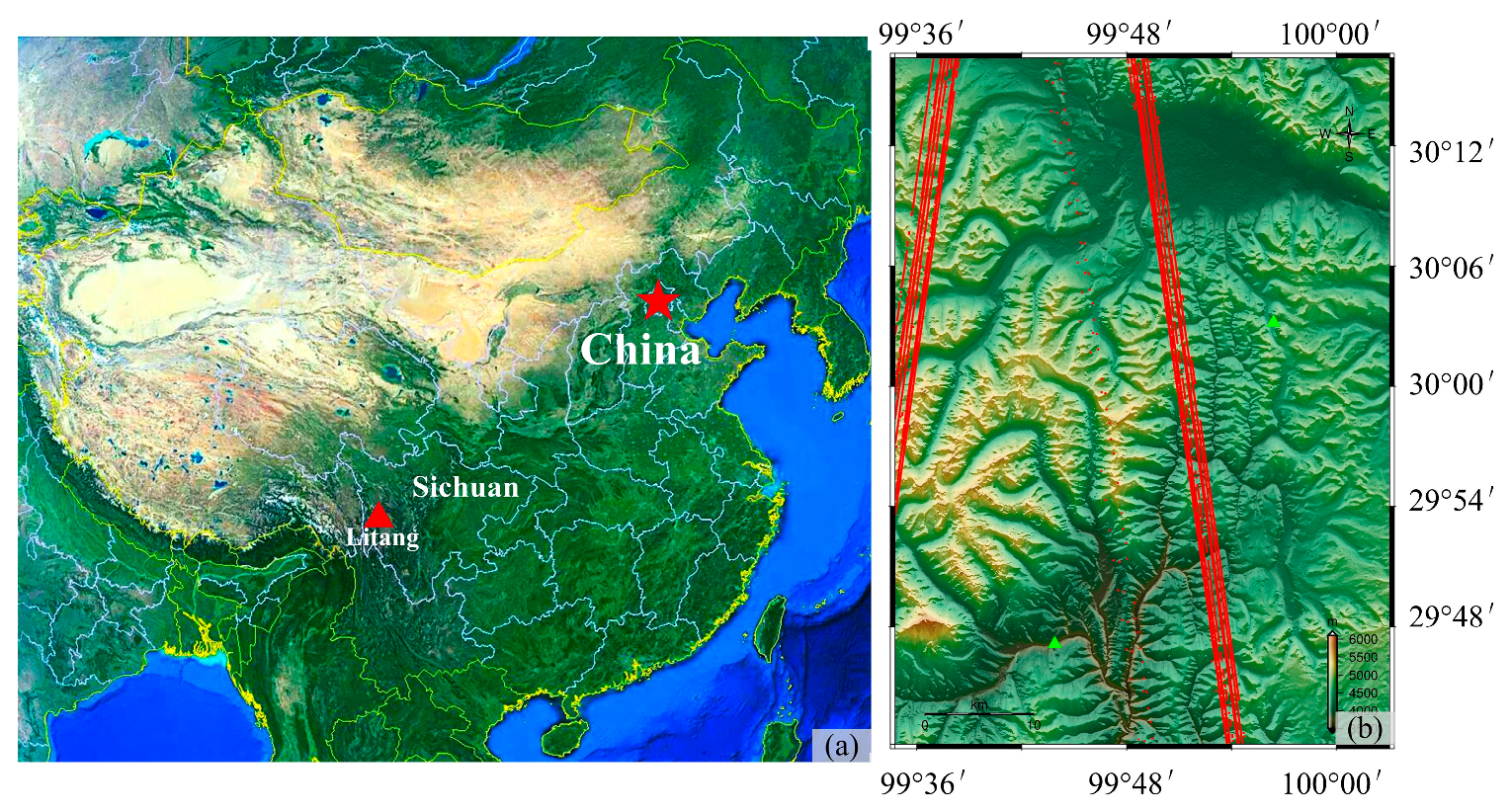
The Ganzi Tibetan Autonomous Prefecture of Sichuan province, China, is located in the transition area from the Sichuan Basin to the Tibetan Plateau. This area is highly undulated. The height difference between the northern plateau and southern valley is about 3000 m, and that between the Gongga Mountain, the tallest mountain in the area, and the Dadu River Valley is 6400 m. A location map of the study area and the corresponding SRTM DEM are shown in Figure 9. We select the corresponding ICESat data and two ground control points for accuracy evaluation. It is worth noting that the elevation systems of SRTM and of the control points are of orthometric height, referring to the Earth Gravitational Model reference 1996 (EGM96). The TanDEM and ICESat use the ellipsoid height, referring to the World Geodetic System 1984 (WGS84) ellipsoid [43]. For convenience and consistency, all data are transformed to the orthometric height system.
Because the height difference in the study area is as large as 2600 m, the 8 × 8 multi-look processing without external DEM introduces large phase unwrapping error, leading to a final DEM error of 310 m. We need to employ SRTM to reduce the EPG. In order to ensure the processing precision, SRTM DEM should be properly oversampled to get a grid size approximating to the TSX/TDX pixel size after multi-look processing. Then we have to co-register them and make sure the accuracy in range and azimuth directions do not exceed 1 pixel.
Multi-look 8 × 8 processing is able to suppress interferometric phase noise in our study. If we apply the external SRTM data to decrease EPG, the final phase gradient will be small enough to provide reasonable CDEM data with few details. CDEM will be useful to provide quick view of the DEM results, but its terrain details cannot meet the requirements of high-precision production.
We need to take the CDEM as a reference in the 4 × 4 multi-look processing to ensure the reliability of phase unwrapping. To reduce error propagation in the iteration process, low coherent regions with large NLs are firstly masked, and then interpolated with cubic convolution. This kind of processing improves the reliability of elevation in the decorrelation regions and the elevation continuity all over the interferogram, avoiding phase unwrapping error in subsequent steps. The IDEM generated by 4 × 4 multi-look processing is only used to control error propagation.
Multi-look 2 × 2 processing provides the final DEM data. As the phase noise cannot be suppressed effectively under this circumstance, the allowable elevation phase gradient is small, thereby direct solution will seriously lower the quality of the results. In this experiment, with the real TanDEM-X data, the DEM accuracy obtained using NL of 2 × 2 is 13.6 m (w.r.t. GCPs), while it can be 1.73 m (w.r.t. GCPs) when the proposed method is used. Meanwhile, assessment using ICESat data also demonstrates the effectiveness of the multi-look iteration algorithm. As Table 1 shows, the elevation accuracy of ICESat data is slightly higher than that of SRTM in complicated terrain regions.
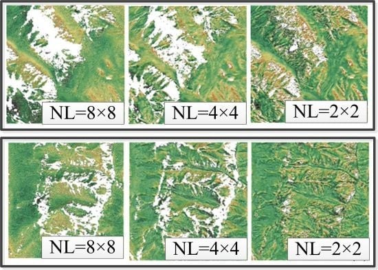
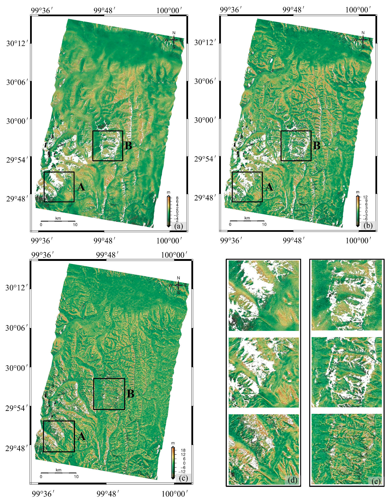
It is conceivable that TanDEM DEM becomes more consistent with real terrain information when NL becomes smaller. And differences between TanDEM DEM and SRTM increase simultaneously. In Figure 10a, we can see some terrain discrepancies, among which the difference between ridge and valley is not obvious. In Figure 10b, obvious textures appear. Figure 10c shows not only clear texture information of the ridge and valley, but also the fine texture among mountains. These results indicate that TanDEM DEM has high potential to provide extremely fine textures where SRTM fails. In addition, we mask the error distribution map using a coherence threshold of 0.9 and show the low coherent regions in white (Figure 10). We can read from Figure 10 that when NL is large, the EPG is great, and phase consistency as well as coherence are low, and vice versa. Figure 10d,e show the enlarged view of regions A and B. The percent of low-coherent areas decrease from 5.38% to 3.14% and 0.43% for NLs of 8 × 8, 4 × 4, and 2 × 2, respectively. And the corresponding statistics are 1.82%, 1.50%, and 0.04% in region B. These results indicate that the proposed multi-look iteration algorithm is useful for calculating DEMs with both high accuracy and fine detail.
5. Discussion
The proposed multi-look iteration algorithm uses NLs of 8 × 8, 4 × 4, and 2 × 2. Other looks are also applicable in the processing chains but the accuracy is not obviously improved. We take experiments using NLs of , and compare the results with the proposed method with NLs of 8 × 8, 4 × 4, and 2 × 2. The first strategy shows that accuracy assessed using GCPs and ICESat data mainly increases when the iteration goes on. But, the relationship between DEM accuracy and NLs is not linear or describable by any functions. This kind of randomness originates from phase unwrapping errors which exist as the random errors in InSAR processing [41]. Thereafter, the uncertainties of unwrapped phase propagate to the final elevation and positioning values. We compare the RMSEs obtained from the first strategy and the proposed strategy. Our results show that the first strategy exhibits worse accuracy if assessed using GCPs, while better if assessed using SRTM and ICESat. That means if we select the first strategy, TanDEM-X DEM is more similar to the data obtained by using large posting (90 m for SRTM, and 70 m for ICESat), but is more different from the real data, i.e., GCPs. That is not our expectation. Take 4 × 4 for example, RMSEs calculated from GCPs in the first strategy is 2.20 m, while that in the second strategy is 2.13 m. RMSEs obtained using SRTM are 4.07 and 4.84 m, respectively. And RMSEs from ICESat are 4.25 m and 4.55 m. Therefore, if more intermediate NLs are used for other purpose during multi-look iteration, we have to take care of the error propagation. Besides, we conduct experiments using just 8 × 8 and 2 × 2 NLs, ignoring the IDEM. The final DEM is 4.22 m, which is worse than that (1.73 m) of applying IDEM. So we suggest use three steps as proposed in the paper to finish the algorithm.
One of the most severe problems besides phase unwrapping is geocoding. Although TDX is precisely calibrated and the positioning accuracy is declared to be around 0.3 m [44], we still find that the geolocation of the images are not consistent between the TSX and TDX images of a coregistered single look slant range complex (CoSSC) product. Therefore the images are all coregistered to a reference SRTM with a threshold 1 pixel in both azimuth and range directions to avoid geocoding error. This is feasible for most of the NLs except 2 × 2. We can read from Figure 6 that NLs 2 × 2 could not decrease the noise obviously. Speckle noise contaminates the robustness of homologous point’s detection. We have to over-sample SRTM data 45 times to meet the pixel spacing of TanDEM-X. But, oversampling brings no extra information, meaning that nearly no texture could be detected within a window of 45 × 45 pixels. Enlarging the window size decreases the processing efficiency and gives barely any help to increase the number and robustness of the homologous points. A practicable way to solve the problem is to use the co-registration polynomial extracted from 4 × 4 NL by considering both the NL and the resampling factor of SRTM.
DLR provides DEMs with different accuracy and resolutions. The accuracy of standard global DEMs is 2 m following the posting of 12 m, which is defined by high resolution terrain information-3 (HRTI-3). Other products such as 4 m @ 6 m (accuracy @ posting), 1 m @ 25 m and 0.5 m @ 50 m are also available under special requests [45]. NLs of 3 × 3 might be used if the posting of DEM is set to 6 m. While that of 12 m refers to NL of 6 × 6. When DEMs go coarse, large NLs are not applicable because of height phase distortion in the undulated regions. Therefore, an applicable way to create DEM products with higher accuracy but coarse resolution is to down-sample the fine DEM. The simulated coarse DEM in our experiment is created using this way. The down-sampling method averages several pixels using different weights, thus weakening the stochastic characteristics of the terrain as expressed in the fBm model, and improve the statistical quality of the DEM. We can tell from the production types of DLR that there is discrepancy between high accuracy and small posting. In this paper, the proposed method is able to ease the conflict. We can create DEMs with both high accuracy and small posting. The pixel spacing of the DEM data could be as small as 4 m with accuracy better than 2 m.
However, some problems still need further study, such as co-registration between ICESat and TanDEM-X, interferometric calibration with sparse GCPs, and the data processing strategy of low coherent regions. The authors are working on the problems and hope to solve them in the near future.
6. Conclusions
This paper presents an InSAR multi-look iteration algorithm to generate DEMs with both high accuracy and fine details. Large NLs are used to suppress noise and produce CDEMs with few details. Small NLs are then applied with reference to CDEMs to avoid height phase distortion and calculate DEMs with fine textures and high accuracy. The largest NL that can be adopted is 8 × 8, under which situation all the noise is suppressed. The smallest NL is 2 × 2 to ensure that the noise phase gradient is less than the maximum detectable phase gradient. An intermediate NL of 4 × 4 is suggested to control error propagation.
The fBm model is used to conduct simulated experiments. Results indicate that when the height range is 2000 m, the proposed method is able to provide DEMs with accuracy of 2.10 m, better than the accuracy of 2.33 m which is obtained using traditional method. When the height range increases to 2600 m, phase unwrapping error induces great error and use of an external DEM is advised to decrease the elevation phase gradient and ensure the phase unwrapping accuracy. The height accuracy could be 3.48 m after multi-look iteration analysis.
The TanDEM-X images are used to test the feasibility of the algorithm. One of the most undulated regions is selected to conduct the experiment. The Litang County of Ganzi Tibetan Autonomous Prefecture of Sichuan province, China, is located in the transition area from the Sichuan Basin to the Tibetan Plateau. The height range of the county is about 2600 m. If no external DEM is used, phase unwrapping introduces 310 m height error. Therefore SRTM DEM is applied and 8 × 8 NL decreases the error from 310 m to 2.36 m. The accuracy of IDEM generated by 4 × 4 NL is 2.13 m. While that of 2 × 2 NL is 1.73 m. By comparing the differences between SRTM and TanDEM-X DEM, we are able to tell that TanDEM-X is highly capable of providing both high accuracy and abundant details. The proposed method can be used to create a DEM product with accuracy of 1.73 m and posting of 4 m.
Acknowledgments
This work was supported by National Key R&D Programme of China (No: 2017YFB0502700), Civilian Space Programme of China (No: D010102), National Basic Surveying and Mapping Science and Technology Plan (No: 2016KJ0204/2017KJ0204/2017KJ0304), Non Profit Industry Research Subject (No: 201512022). The authors would like to thank German Aerospace Center (DLR) for providing TanDEM-X data (No: CAL_VAL6993).
Author Contributions
Yaolin Liu and Tao Li are the two main reviewers of the manuscript. Yaolin Liu is the corresponding author and spends much time providing suggestions on the organization of the paper. Tao Li contributes the prototype idea of the paper. Danqin Wu helps process the simulated data and assesses the results.
Conflicts of Interest
The authors declare no conflict of interest.
References
- Massonnet, D.; Elachi, C. High-resolution land topography. C. R. Geosci. 2006, 338, 1029–1041. [Google Scholar] [CrossRef]
- Ferretti, A.; Prati, C.; Rocca, F. Permanent scatterers in SAR interferometry. IEEE Trans. Geosci. Remote Sens. 2001, 39, 8–20. [Google Scholar] [CrossRef]
- Liu, G.; Jia, H.; Nie, Y.; Li, T.; Zhang, R.; Yu, B.; Li, Z. Detecting subsidence in coastal areas by ultrashort-baseline TCPInSAR on the time series of high-resolution TerraSAR-X images. IEEE Trans. Geosci. Remote Sens. 2014, 52, 1911–1923. [Google Scholar]
- Tomás, R.; Li, Z. Earth Observations for Geohazards: Present and Future Challenges. Remote Sens. 2017, 9, 194. [Google Scholar] [CrossRef]
- Massonnet, D.; Rossi, M.; Carmona, C.; Adragna, F.; Peltzer, G.; Feigl, K.; Rabaute, T. The displacement field of the Landers earthquake mapped by radar interferometry. Nature 1993, 364, 138–142. [Google Scholar] [CrossRef]
- Zebker, H.A.; Rosen, P.A.; Goldstein, R.M.; Gabriel, A.; Werner, C.L. On the derivation of coseismic displacement fields using differential radar interferometry: The Landers earthquake. J. Geophys. Res. Solid Earth 1994, 99, 19617–19634. [Google Scholar] [CrossRef]
- Dai, K.; Li, Z.; Tomás, R.; Liu, G.; Yu, B.; Wang, X.; Cheng, H.; Chen, J.; Stockamp, J. Monitoring activity at the Daguangbao mega-landslide (China) using Sentinel-1 TOPS time series interferometry. Remote Sens. Environ. 2016, 186, 501–513. [Google Scholar] [CrossRef]
- Scaioni, M. Remote Sensing for Landslide Investigations: From Research into Practice. Remote Sens. 2013, 5, 5488–5492. [Google Scholar] [CrossRef]
- Rogers, A.E.E.; Ingalls, R.P. Venus: Mapping the Surface Reflectivity by Radar Interferometry. Science 1969, 165, 797–799. [Google Scholar] [CrossRef] [PubMed]
- Zisk, S.H. A new, earth-based radar technique for the measurement of lunar topography. Moon 1972, 4, 296–306. [Google Scholar] [CrossRef]
- Graham, L.C. Synthetic interferometer radar for topographic mapping. Proc. IEEE 1974, 62, 763–768. [Google Scholar] [CrossRef]
- Farr, T.G.; Rosen, P.A.; Caro, E.; Crippen, R.; Duren, R.; Hensley, S.; Kobrick, M.; Paller, M.; Rodriguez, E.; Roth, L.; et al. The Shuttle Radar Topography Mission. Rev. Geophys. 2007, 45, 1–33. [Google Scholar] [CrossRef]
- Buckreuβ, S. TerraSAR-X/TanDEM-X Mission Overview. In Proceedings of the TerraSAR-X/TanDEM-X Science Meeting, Oberpfaffenhofen, Oberpfaffenhofen, Germany, 17–20 October 2016. [Google Scholar]
- Krieger, G.; Moreira, A.; Fiedler, H.; Hajnsek, I.; Werner, M.; Younis, M.; Zink, M. TanDEM-X: A satellite formation for high-resolution SAR interferometry. IEEE Trans. Geosci. Remote Sens. 2007, 45, 3317–3341. [Google Scholar] [CrossRef] [Green Version]
- Schwerdt, M.; Gonzalez, J.H.; Bachmann, M.; Schrank, D.; Döring, B.; Ramon, N.T.; Antony, J.M.W. In-Orbit Calibration of the TanDEM-X System. In Proceedings of the 2011 IEEE International Geoscience and Remote Sensing Symposium (2011 IGARSS), Vancouver, BC, Canada, 24–29 July 2011; pp. 2420–2423. [Google Scholar]
- Gruber, A.; Wessel, B.; Huber, M.; Roth, A. Operational TanDEM-X DEM calibration and first validation results. ISPRS J. Photogramm. 2012, 73, 39–49. [Google Scholar] [CrossRef]
- González, J.H.; Antony, J.M.W.; Bachmann, M.; Krieger, G.; Zink, M.; Schrank, D.; Schwerdt, M. Bistatic system and baseline calibration in TanDEM-X to ensure the global digital elevation model quality. ISPRS J. Photogramm. 2012, 73, 3–11. [Google Scholar] [CrossRef]
- Gruber, A.; Wessel, B.; Martone, M.; Roth, A. The TanDEM-X DEM mosaicking: Fusion of multiple acquisitions using InSAR quality parameters. IEEE J. Sel. Top. Appl. Earth Obs. 2015, 9, 1047–1057. [Google Scholar] [CrossRef]
- Martone, M.; Bräutigam, B.; Rizzoli, P.; Gonzalez, C.; Bachmann, M.; Krieger, G. Coherence evaluation of TanDEM-X interferometric data. ISPRS J. Photogramm. 2012, 73, 21–29. [Google Scholar] [CrossRef] [Green Version]
- Hanssen, R.F. Radar Interferometry: Data Interpretation and Error Analysis; Springer Science & Business Media: Berlin, Germany, 2001; p. 314. [Google Scholar]
- Richard, B.; Philipp, H. Synthetic aperture radar interferometry. Inverse Prob. 1998, 14, R1–R54. [Google Scholar]
- Jiang, M.; Li, Z.W.; Ding, X.L.; Zhu, J.J.; Feng, G.C. Modeling minimum and maximum detectable deformation gradients of interferometric SAR measurements. Int. J. App. Earth Obs. 2011, 13, 766–777. [Google Scholar] [CrossRef]
- Guarnieri, A.M. Using topography statistics to help phase unwrapping. IEE Proc. Radar Sonar Navig. 2003, 150, 144–151. [Google Scholar] [CrossRef]
- Gruber, A.; Wessel, B.; Huber, M. TanDEM-X DEM Calibration: Correction of systematic DEM errors by block adjustment. In Proceedings of the IEEE International Geoscience and Remote Sensing Symposium (IGARSS 2009), Cape Town, South Africa, 12–17 July 2009; pp. II-761–II-764. [Google Scholar]
- Hanssen, R.F.; Weckwerth, T.M.; Zebker, H.A.; Klees, R. High-resolution water vapor mapping from interferometric radar measurements. Science 1999, 283, 1297–1299. [Google Scholar] [CrossRef] [PubMed]
- Touzi, R.; Lopes, A. Statistics of the Stokes parameters and of the complex coherence parameters in one-look and multilook speckle fields. IEEE Trans. Geosci. Remote Sens. 1996, 34, 519–531. [Google Scholar] [CrossRef]
- Bezvesiniy, O.O.; Gorovyi, I.M.; Vavriv, D.M. Effects of local phase errors in multi-look SAR images. Prog. Electromagn. Res. B 2013, 53, 1–24. [Google Scholar] [CrossRef]
- Jong-Sen, L.; Hoppel, K.W.; Mango, S.A.; Miller, A.R. Intensity and phase statistics of multilook polarimetric and interferometric SAR imagery. IEEE Trans. Geosci. Remote Sens. 1994, 32, 1017–1028. [Google Scholar] [CrossRef]
- Chen, C.W.; Zebker, H.A. Phase unwrapping for large SAR interferograms: statistical segmentation and generalized network models. IEEE Trans. Geosci. Remote Sens. 2002, 40, 1709–1719. [Google Scholar] [CrossRef]
- Zebker, H.A.; Goldstein, R.M. Topographic mapping from interferometric synthetic aperture radar observations. J. Geophys. Res. Solid Earth 1986, 91, 4993–4999. [Google Scholar] [CrossRef]
- Goldstein, R.M.; Zebker, H.A.; Werner, C.L. Satellite radar interferometry: Two-dimensional phase unwrapping. Radio Sci. 1988, 23, 713–720. [Google Scholar] [CrossRef]
- Danudirdjo, D.; Hirose, A. Anisotropic phase unwrapping for synthetic aperture radar interferometry. IEEE Trans. Geosci. Remote Sens. 2015, 53, 4116–4126. [Google Scholar] [CrossRef]
- Marechal, N. Tomographic formulation of interferometric SAR for terrain elevation mapping. IEEE Trans. Geosci. Remote Sens. 1995, 33, 726–739. [Google Scholar] [CrossRef]
- Lombardini, F.; Pardini, M. Superresolution Differential Tomography: Experiments on Identification of Multiple Scatterers in Spaceborne SAR Data. IEEE Trans. Geosci. Remote Sens. 2012, 50, 1117–1129. [Google Scholar] [CrossRef] [Green Version]
- Ma, P.; Lin, H. Robust detection of single and double persistent scatterers in urban built environments. IEEE Trans. Geosci. Remote Sens. 2015, 54, 2124–2139. [Google Scholar] [CrossRef]
- Berardino, P.; Fornaro, G.; Lanari, R.; Sansosti, E. A new algorithm for surface deformation monitoring based on small baseline differential SAR interferograms. IEEE Trans. Geosci. Remote Sens. 2002, 40, 2375–2383. [Google Scholar] [CrossRef]
- Ferretti, A.; Fumagalli, A.; Novali, F.; Prati, C.; Rocca, F.; Rucci, A. A new algorithm for processing interferometric data-stacks: SqueeSAR. IEEE Trans. Geosci. Remote Sens. 2011, 49, 3460–3470. [Google Scholar] [CrossRef]
- Chen, C.W. Statistical-Cost Network-Flow Approaches to Two-Diminsional Phase Unwrapping for RADAR Interferometry. Ph.D. Thesis, Stanford University, Los Angeles, CA, USA, 2001; p. 159. [Google Scholar]
- Bamler, R.; Adam, N.; Davidson, G.W.; Just, D. Noise-induced slope distortion in 2-D phase unwrapping by linear estimators with application to SAR interferometry. IEEE Trans. Geosci. Remote Sens. 1998, 36, 913–921. [Google Scholar] [CrossRef]
- Baran, I.; Stewart, M.; Claessens, S. A new functional model for determining minimum and maximum detectable deformation gradient resolved by satellite radar interferometry. IEEE Trans. Geosci. Remote Sens. 2005, 43, 675–682. [Google Scholar] [CrossRef]
- Elachi, C. Spaceborne Radar Remote Sensing: Applications and Techniques; Institute of Electical and Electornics Engineers: New York, NY, USA, 1988; p. 285. [Google Scholar]
- Kaplan, L.M.; Kuo, C.C.J. An improved method for 2-D self-similar image synthesis. IEEE T. Image Process. 1996, 5, 754–761. [Google Scholar] [CrossRef] [PubMed]
- Li, P.; Li, Z.; Shi, C.; Feng, W.; Liang, C.; Li, T.; Zeng, Q.; Liu, J. Impact of geoid height on large-scale crustal deformation mapping with InSAR observations. Chin. J. Geophys. 2016, 56, 1857–1867. (In Chinese) [Google Scholar]
- Fritz, T.; Breit, H.; Lachaise, M.; Rossi, C.; Yague-Martinez, N. In Processing Strategies for Global Interferometric TanDEM-X DEM Generation. In Proceedings of the 10th European Conference on Synthetic Aperture Radar, Berlin, Germany, 3–5 June 2014; pp. 1–4. [Google Scholar]
- Kosmann, D.; Wessel, B.; Schwieger, V. Global Digital Elevation Model from TanDEM-X and the Calibration/Validataion with Worldwide Kinematic GPS-Tracks. In Proceedings of the XXIV FIG International Congress, Sydney, Australia, 11–16 April 2010. [Google Scholar]
Figure 1.
Relationship between pixel spacing and the probability density distribution function of elevation gradients in (a) the range direction and (b) the azimuth direction. Lines are the pixel spacing with different multi-look numbers.
Figure 1.
Relationship between pixel spacing and the probability density distribution function of elevation gradients in (a) the range direction and (b) the azimuth direction. Lines are the pixel spacing with different multi-look numbers.

Figure 2.
(a–c) Noise phase probability density functions with different coherences and number of looks. The coherence is 0.7, 0.8, and 0.9, respectively. The multi-look numbers of the blue, red, and black lines are 64, 16, and 4, respectively.
Figure 2.
(a–c) Noise phase probability density functions with different coherences and number of looks. The coherence is 0.7, 0.8, and 0.9, respectively. The multi-look numbers of the blue, red, and black lines are 64, 16, and 4, respectively.

Figure 3.
(a–c) Probability density function of interferometric noise phase gradient with different coherence and number of looks. The coherence is 0.7, 0.8, and 0.9, respectively. The multi-look numbers of the blue, red, and black lines are 64, 16, and 4.
Figure 3.
(a–c) Probability density function of interferometric noise phase gradient with different coherence and number of looks. The coherence is 0.7, 0.8, and 0.9, respectively. The multi-look numbers of the blue, red, and black lines are 64, 16, and 4.


Figure 4.
Relationship among the number of looks, the maximum detectable phase gradient, and the noise phase gradient.
Figure 4.
Relationship among the number of looks, the maximum detectable phase gradient, and the noise phase gradient.

Figure 5.
(a) is DEM simulated using fractional Brownian motion, the white rectangle corresponds to (b) the spatial coverage of SLC image.
Figure 5.
(a) is DEM simulated using fractional Brownian motion, the white rectangle corresponds to (b) the spatial coverage of SLC image.

Figure 6.
Relationship between number of looks and the mean values of absolute height phase gradient, absolute noise phase gradient, and absolute phase gradient.
Figure 6.
Relationship between number of looks and the mean values of absolute height phase gradient, absolute noise phase gradient, and absolute phase gradient.

Figure 7.
(a–c) Relationship between the height accuracy and the mean values of absolute phase gradient, absolute noise phase gradient and absolute phase gradient.
Figure 7.
(a–c) Relationship between the height accuracy and the mean values of absolute phase gradient, absolute noise phase gradient and absolute phase gradient.

Figure 8.
(a–c) Histogram of elevation error. In (a–c) the simulated elevation differences are 2000 m, 2600 m, 3000 m, respectively.
Figure 8.
(a–c) Histogram of elevation error. In (a–c) the simulated elevation differences are 2000 m, 2600 m, 3000 m, respectively.

Figure 9.
(a) Location map of the study area. The red triangle is Litang County, Ganzi Tibetan Autonomous Prefecture, and (b) the corresponding SRTM DEM. The red dots are ICESat data and the two green triangles are the ground control points.
Figure 9.
(a) Location map of the study area. The red triangle is Litang County, Ganzi Tibetan Autonomous Prefecture, and (b) the corresponding SRTM DEM. The red dots are ICESat data and the two green triangles are the ground control points.

Figure 10.
Elevation error map (w.r.t SRTM) with NLs of (a) 8 × 8, (b) 4 × 4, and (c) 2 × 2. We zoom in the rectangular regions of A and B and show the corresponding results in (d,e). White regions within the error map are pixels with coherence lower than 0.9.
Figure 10.
Elevation error map (w.r.t SRTM) with NLs of (a) 8 × 8, (b) 4 × 4, and (c) 2 × 2. We zoom in the rectangular regions of A and B and show the corresponding results in (d,e). White regions within the error map are pixels with coherence lower than 0.9.


Table 1.
RMSEs of TanDEM-X DEM assessed using different kinds of reference data (in unit: meters).
| Number of Looks | SRTM | ICESat | GCP |
|---|---|---|---|
| 8 × 8 | 2.82 | 5.88 | 2.36 |
| 4 × 4 | 4.84 | 4.82 | 2.13 |
| 2 × 2 | 6.96 | 4.55 | 1.73 |
© 2017 by the authors. Licensee MDPI, Basel, Switzerland. This article is an open access article distributed under the terms and conditions of the Creative Commons Attribution (CC BY) license (http://creativecommons.org/licenses/by/4.0/).
Share and Cite
MDPI and ACS Style
Gao, X.; Liu, Y.; Li, T.; Wu, D. High Precision DEM Generation Algorithm Based on InSAR Multi-Look Iteration. Remote Sens. 2017, 9, 741. https://0-doi-org.brum.beds.ac.uk/10.3390/rs9070741
AMA Style
Gao X, Liu Y, Li T, Wu D. High Precision DEM Generation Algorithm Based on InSAR Multi-Look Iteration. Remote Sensing. 2017; 9(7):741. https://0-doi-org.brum.beds.ac.uk/10.3390/rs9070741
Chicago/Turabian StyleGao, Xiaoming, Yaolin Liu, Tao Li, and Danqin Wu. 2017. "High Precision DEM Generation Algorithm Based on InSAR Multi-Look Iteration" Remote Sensing 9, no. 7: 741. https://0-doi-org.brum.beds.ac.uk/10.3390/rs9070741
Note that from the first issue of 2016, this journal uses article numbers instead of page numbers. See further details here.