Azimuth Ambiguities Removal in Littoral Zones Based on Multi-Temporal SAR Images

Abstract

Synthetic aperture radar (SAR) is one of the most important techniques for ocean monitoring. Azimuth ambiguities are a real problem in SAR images today, which can cause performance degradation in SAR ocean applications. In particular, littoral zones can be strongly affected by land-based sources, whereas they are usually regions of interest (ROI). Given the presence of complexity and diversity in littoral zones, azimuth ambiguities removal is a tough problem. As SAR sensors can have a repeat cycle, multi-temporal SAR images provide new insight into this problem. A method for azimuth ambiguities removal in littoral zones based on multi-temporal SAR images is proposed in this paper. The proposed processing chain includes co-registration, local correlation, binarization, masking, and restoration steps. It is designed to remove azimuth ambiguities caused by fixed land-based sources. The idea underlying the proposed method is that sea surface is dynamic, whereas azimuth ambiguities caused by land-based sources are constant. Thus, the temporal consistence of azimuth ambiguities is higher than sea clutter. It opens up the possibilities to use multi-temporal SAR data to remove azimuth ambiguities. The design of the method and the experimental procedure are based on images from the Sentinel data hub of Europe Space Agency (ESA). Both Interferometric Wide Swath (IW) and Stripmap (SM) mode images are taken into account to validate the proposed method. This paper also presents two RGB composition methods for better azimuth ambiguities visualization. Experimental results show that the proposed method can remove azimuth ambiguities in littoral zones effectively.

1. Introduction

Synthetic Aperture Radar (SAR) is a microwave remote sensing technology providing 2D images with 24-h all-weather sensing capability [1]. Since the launch of the Seasat in 1978, the number of spaceborne SAR sensors has drastically increased [2,3]. It is a mature and successful discipline for global ocean monitoring [3,4,5,6]. Advanced spaceborne SAR sensors today provide fine resolutions, such as TerraSAR-X, COSMOS-SkyMed, RADARSAT-2, GF-3, and Sentinel-1 [4,5,6,7,8,9]. As more than 90% of the world’s trade goods, and more than 70% of global crude oil are transported by sea, maritime surveillance is of utmost importance [10].

Azimuth ambiguities are inherent artifacts in current SAR systems. They are visible in most spaceborne SAR images. SAR images often suffer from azimuth ambiguities. Experience shows that azimuth ambiguities are today a real problem for ocean monitoring [11,12]. SAR images can be strongly affected by land-based sources. If azimuth ambiguities are unrecognized, they can give rise to false alarms and errors in SAR image interpretation.

Littoral zones are ‘hard-hit areas’ of azimuth ambiguities. There are three reasons for this. The first one is that littoral zones are usually areas of low wind speed condition. The neighboring land can provide a barrier to generate a weak-wind region. Azimuth ambiguities become prominent when the calm sea surface appears darker. The second one is that there are always strong sources at the coast. Coastal regions are always the most developed areas, e.g., New York, Shanghai, Singapore, etc. There are many tall buildings, bridges, ports, and other artifacts. They are all strong sources which can generate azimuth ambiguities. The final one is that the typical spaceborne azimuth ambiguity displacements are 4~8 km. Azimuth ambiguities of land-based sources will occur exactly in sea areas near the coast. Unfortunately, littoral zones are also regions of interest (ROI) in most cases. There are many ships in the harbors, straits, and other important littoral zones usually. The pressure on the security of the ocean is also increasing as shipping traffic grows. Littoral zones bear the brunt of the pressure. They are exposed to various hazards like pollution, terrorism, or privacy. Thus, efficient methods for monitoring, prediction, and visualization of littoral zones are of great importance.

Many investigations have been carried out for azimuth ambiguities removal in SAR imagery. The postprocessing techniques which this paper focuses on can be divided into three categories based on SAR data type used, i.e., methods based on detected (intensity/amplitude) products, single-look complex (SLC) products, and quad-pol (QP) products. Calculating the azimuth displacement to identify azimuth ambiguities is one of the most important methods used in detected products [4,12,13]. This method checks whether there is a stronger source target present at the azimuth displacement. If either side has a detection of stronger power than the source target, it is considered to be an ambiguity. As SLC or QP products can be used to construct detected products, detected products are more common than other type of products. Generally this method is one of the most tractable methods, especially for azimuth ambiguities caused by ship targets. It has been widely used in existed SAR ship detection systems [4,13]. However this method fails to discard azimuth ambiguities when the source is flooded by strong targets in littoral zones or outside of the image. Besides, azimuth ambiguities have unpredictable variations leading to a difficult correlation between sources and ambiguities. Finally, azimuth displacements can be different in ScanSAR or TOPSAR (Terrain Observation with Progressive Scans SAR) images. Methods based on SLC products usually adopt filtering techniques in the frequency domain [14,15], and remove azimuth ambiguities by filtering azimuth signals. They can take advantage of both real and imagery parts in SLC products. Filtering is effective in suppressing azimuth ambiguities, but can result in additional speckle noise and small ship loss. Methods based on QP products employ the fact that the two cross-polarized channels are each other’s complex conjugate for azimuth ambiguities [16]. They consider that a proper combination of two cross-polarized channels [17] or polarimetric decomposition can cancel out azimuth ambiguities [18]. Methods based on QP products are quite effective, whereas QP products are not available in practice usually.

The increasing of multi-temporal SAR images today provides new insight into this problem. For example, Sentinel-1 has a repeat cycle of 12 days by one satellite and 6 days by a pair of satellites [8,19]. A scene on the littoral zones can be re-imaged every 12 days or 6 days. Thus, image pixels of the same scene can be made to exactly coincide. This can identify fixed artifacts in littoral zones. This paper opens up the possibilities to use multi-temporal SAR data to remove azimuth ambiguities. A method for azimuth ambiguities removal in littoral zones based on multi-temporal SAR images is proposed in this paper. The proposed processing chain includes co-registration, local correlation, binarization, masking, and restoration steps applied to images. It is designed to remove azimuth ambiguities caused by fixed land-based sources in littoral zones. The basic idea underlying the proposed method is that the sea surface is dynamic whereas azimuth ambiguities caused by land-based sources are constant. The temporal consistence of azimuth ambiguities is higher than sea clutter. Thus, azimuth ambiguities can be identified by the correlation of multi-temporal SAR images. The design of the method and the experimental procedure are based on detected products from the Sentinel data hub of Europe Space Agency (ESA) [8]. Both Interferometric Wide Swath (IW) and Stripmap (SM) mode images are taken into account to validate the algorithms. Experimental results show that the proposed method can remove azimuth ambiguities in littoral zones effectively when no QP data is available. To obtain better visual results of azimuth ambiguities than original images, this paper also presents two RGB composition methods for azimuth ambiguities based on the number of multi-temporal SAR images available.

The rest of this paper is organized as follows. Section 2 is a review on azimuth ambiguities. Section 3 proposes the method for azimuth ambiguities removal in littoral zones based on multi-temporal SAR images. Section 4 presents two RGB composition methods for azimuth ambiguities. Section 5 validates and discusses the method proposed in this paper by testing on Sentinel-1 IW and SM images. Finally, Section 6 concludes this paper.

2. Review on Azimuth Ambiguities

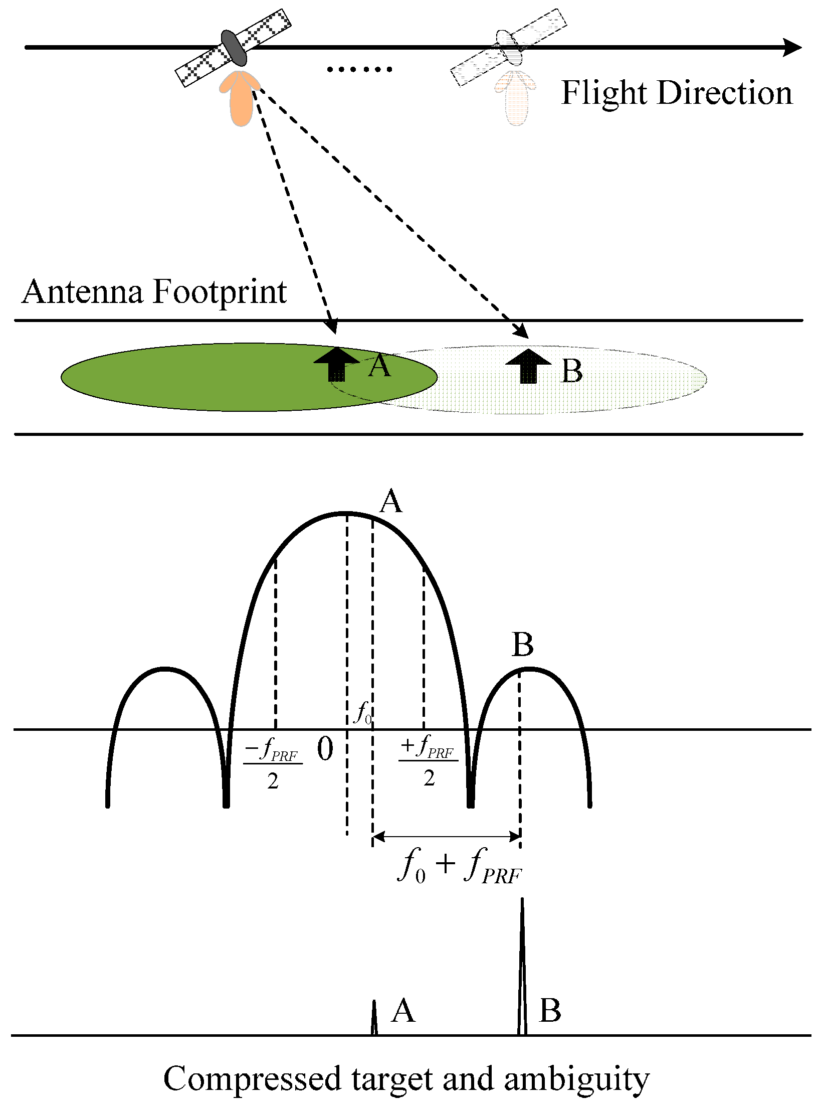
Azimuth ambiguities are caused by finite sampling of azimuth Doppler signals. A too low pulse repetition frequency ($\mathrm{PRF}$) may cause those Doppler frequencies higher than $\mathrm{PRF}$ are folded into the central part of the azimuth spectrum. Thus, aliased signals are produced in this case [17]. As shown in Figure 1, targets A and B have equal Doppler histories due to aliasing. If target B is much stronger than target A, then it is possible that a ghost image of target B will be visible in the position of A. This ghost is called azimuth ambiguity. The Doppler shift as a function of a pointing error, increases linearly with frequency. Azimuth ambiguities in SAR images are spatially displaced in azimuth directions at approximate locations [11,14], as

$$\Delta D_{AZ}\approx n\frac{f_{PRF}}{f_{DR}}V$$

(1)

where $\Delta D_{AZ}$ is the azimuth displacement, $V$ is the satellite velocity, $f_{PRF}$ is the $\mathrm{PRF}$, $f_{DR}$ is the Doppler rate, $n$ is the order.

As

$$f_{DR}\approx \frac{2V^2}{\lambda R_s}$$

(2)

where $\lambda$ is the wavelength and $R_s$ is the slant range, an equivalent representation of Formula (1) is

$$\Delta D_{AZ}\approx n\frac{\lambda R_s}{2V}{f}_{PRF}$$

(3)

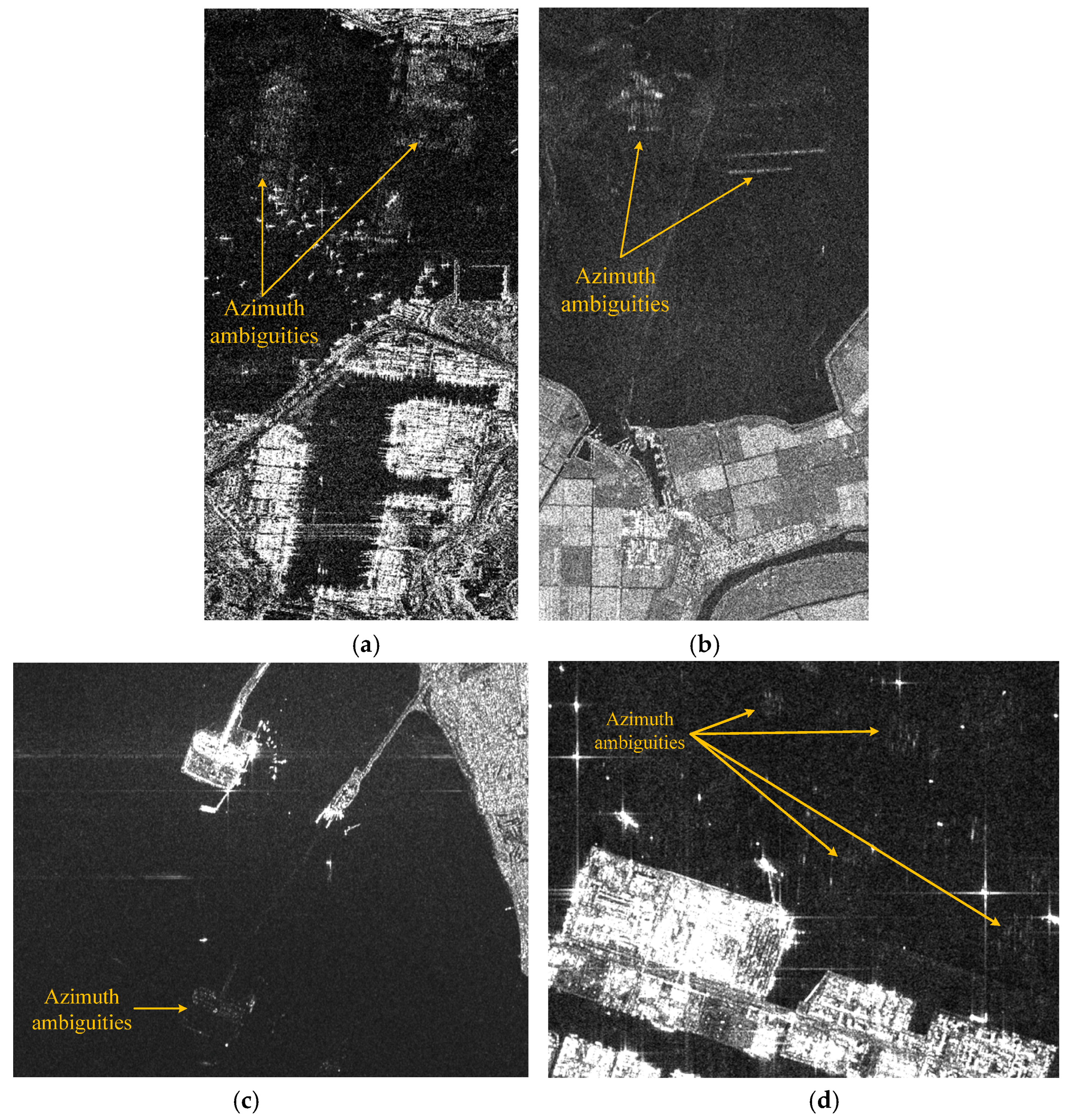
Typical azimuth ambiguity displacements are 4~8 km. In cases where the sea clutter level is low, e.g., weak-wind areas, azimuth ambiguities can occur more easily. A quality measure for azimuth ambiguities is the Azimuth Ambiguity to Signal Ratio (AASR). The requirement of AASR for ship detection and oil spill detection is −25 dB and −23 dB, respectively [12]. Azimuth ambiguities are inherent artifacts in current SAR systems, which appear in most spaceborne SAR images. As shown in Figure 2, azimuth ambiguities and their azimuth displacements in TerraSAR-X, COSMOS-SkyMed, RADARSAT-2, and Sentinel-1 images are presented. Azimuth ambiguities in the littoral zones affect SAR image interpretation severely.

The important features of azimuth ambiguities can be concluded into 5 aspects:

(1)

They occur in azimuth direction at determinate multiple distances at two sides of the source target. They may also have a small shift in range direction. Thus, the theoretical distance can be less than the measured distance.

(2)

The displacement rises as the wavelength increases, other parameters remaining the same. The ambiguities are less severe in SAR images of a long wavelength than a short wavelength.

(3)

As the order $n$ increases, the displacements of the related ambiguities increase and their intensities decrease usually. The power of the 1st order azimuth ambiguity is weaker than the source target.

(4)

They appear to be not well focused or not very strong in intensities. However they are similar to the source target in some features, e.g., shape, texture, size. Thus, it is not easy to identify them by methods based on features.

(5)

HV and VH channels have approximately the same magnitude, whereas their azimuth ambiguities are shifted in phase by about 180°.

3. Proposed Method

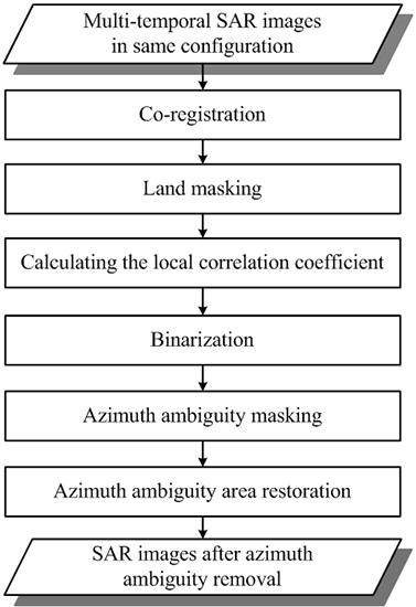
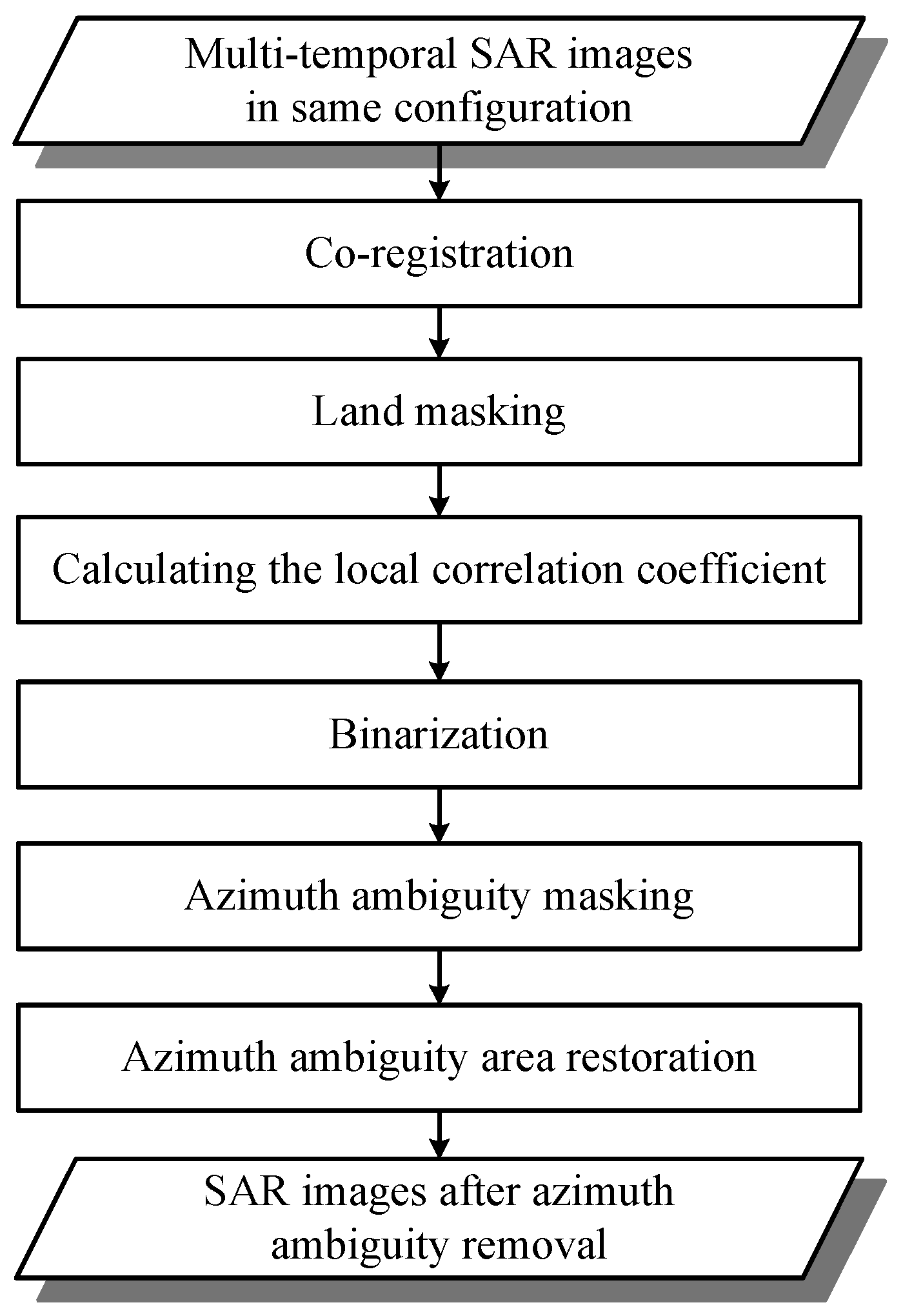
In the proposed method, multi-temporal SAR images of the same scene in the same configuration should be available first. The same configuration indicates that the multi-temporal SAR images should be acquired by a same sensor with same the imaging mode and pass way (ascending or descending) at least. Figure 3 shows the detailed flowchart of the proposed method which can be divided into 6 steps.

3.1. Co-Registration

To support the mapping of multi-temporal SAR images, some relevant preprocessing operations must be performed. These mainly include the co-registration of SAR data. Co-registration is accomplished through cross correlation and warp usually. Then we abstract the same geographical areas from multi-temporal SAR data. Thus, corresponding pixels in multi-temporal SAR images exactly coincide and represent the same point on the Earth surface. It should be noted that radiometric correction and speckle filtering are not needed in the preprocessing. This simplifies the processing chain. The reason will be presented in the subsequent steps.

3.2. Land Masking

As only the ocean is of interest, land masking is important for multi-temporal SAR images. There are two popular approaches for land masking. One is to register SAR images with existing geospatial databases, e.g., the GSHHS (Global Self-consistent, Hierarchical, High-resolution Shoreline) [21]. Another one is to use automatic algorithms to detect coastlines or land areas [22,23]. In this paper, land will be removed for better results in subsequent steps.

3.3. Calculating the Local Correlation Coefficient

As sea surface is dynamic, whereas azimuth ambiguities caused by land-based sources are fixed. The temporal consistence of azimuth ambiguities is higher than sea clutter. Thus, we can use correlation operation to identify azimuth ambiguities from sea clutter. Two-temporal images in the same configuration are needed at least. Generally, more images seem to be better when applying the correlation operation. However there is an increasing risk that land-based sources changed in a long period. Thus, two-temporal images acquired in continuous periods are preferred in this paper.

The local correlation coefficient between each image is calculated in a local sliding window. The size of the sliding window can be decided by a reference size, e.g., the smallest ship one wants to detect. If there are two-temporal images available, named $I_1$, $I_2$, then

$$R=I_1\otimes I_2$$

(4)

where $R$ is the local correlation coefficient map, $\otimes$ indicates the local correlation operation here, i.e.,

$$r=\frac{{\displaystyle \sum _m{\displaystyle \sum _n\left(I_1\left(m,n\right)-{\overline{I}}_1\right)\left(I_2\left(m,n\right)-{\overline{I}}_2\right)}}}{\sqrt{\left({\displaystyle \sum _m{\displaystyle \sum _n{\left(I_1\left(m,n\right)-{\overline{I}}_1\right)}^2}}\right)\left({\displaystyle \sum _m{\displaystyle \sum _n{\left(I_2\left(m,n\right)-{\overline{I}}_2\right)}^2}}\right)}}$$

(5)

where $r$ is the local correlation coefficient value at sliding window center, $I_1\left(m,n\right)$ and $I_2\left(m,n\right)$ are the pixel values at location $\left(m,n\right)$ in the sliding window respectively, ${\overline{I}}_1$ and ${\overline{I}}_2$ are the mean of all pixels in the sliding window respectively.

As azimuth ambiguities are temporally more consistent than sea clutter and ships, the correlation coefficient of azimuth ambiguities are much higher than sea clutter and ships. Thus, azimuth ambiguities and other constant artifacts are prominent in the local correlation coefficient map. Note that the local correlation operation does not need radiometric correction and speckle filtering. The reason is that the correlation operation is applied in a local window. The radiometric scaling can be considered as a constant in a local window, while the correlation operation is invariant to this constant scaling. Meanwhile, speckle filtering reduces granularity in SAR images. This may increase the consistence of sea clutter. Thus, both radiometric correction and speckle filtering are not needed.

3.4. Binarization

Azimuth ambiguities are prominent, whereas sea clutter is suppressed in the local correlation coefficient map. Thus, azimuth ambiguities can be identified by a binarization operation. Binarization can be achieved by a thresholding method. There are many thresholding methods. In this paper, the thresholding method based on maximum entropy [24] is employed. In this method, two probability distributions $h_i{}^{\left(1\right)}$ and $h_i{}^{\left(2\right)}$ (e.g., object and background) are derived from the original gray distribution of the image. If $t$ is the threshold, then the entropy of the object and background are defined as

$$\begin{array}{l}{H}_b=-{\displaystyle \sum _{i=1}^t{h}_i{}^{\left(1\right)}\lg h_i{}^{\left(1\right)}}\\ H_w=-{\displaystyle \sum _{i=t+1}^L{h}_i{}^{\left(2\right)}\lg h_i{}^{\left(2\right)}}\end{array}$$

(6)

where $L$ is the gray level. Then the optimal threshold $t^{*}$ is defined as the gray level, which maximizes $H_b+H_w$, i.e.,

$$t^{*}=\arg \max \left\{H_b\left(t\right)+H_w\left(t\right)\right\}$$

(7)

The idea underlying this entropic method is that the optimal threshold should make the object and background areas more homogenous with each other. This can make sense for the local correlation coefficient map which is like a blurred ‘salt and pepper’ map. It should be noted that Otsu method [25] or Mode method [26] that require two peaks in the histogram are not appropriate in this case as two peaks may not occur in the histogram.

3.5. Azimuth Ambiguity Masking

The binarization result can be considered as an azimuth ambiguity mask. This mask can be used to remove azimuth ambiguities in multi-temporal SAR images. Thus, multi-temporal SAR images are freed from azimuth ambiguities in littoral zones. On the other hand, an azimuth ambiguity mask can also be used to locate the strong land-based sources. It is an inversion of the method by calculating the displacement to identify azimuth ambiguities. The inversion results can also be used to distinguish 1st order azimuth ambiguities and higher order azimuth ambiguities. If the shifted mask is on the land, the mask can be recognized as 1st order azimuth ambiguities. However if the shifted mask is on the sea, the mask can be recognized as higher order azimuth ambiguities or fixed artifacts on the sea. This is because only the mask of 1st order azimuth ambiguities can be shifted on the land by an azimuth displacement.

3.6. Azimuth Ambiguity Area Restoration

Azimuth ambiguities have little help for the ocean environment and maritime traffic monitoring, though Liu, C. et al. [16] mentioned that azimuth ambiguities may indicate moving objects by the subtraction of two cross-polarized channels. Thus, this paper restores the azimuth ambiguity patches masked in the multi-temporal SAR images. If sea clutter is homogeneous, azimuth ambiguity patches are filled with pixels randomly from a Gaussian distribution. The parameters of the Gaussian distribution are estimated from sea clutter based on methods of moments. If sea clutter is heterogeneous, given the complex textures and structures, the Exemplar-based inpainting method [27] is employed for filling the lost patches of images. The homogeneity is estimated by the equivalent number of looks (ENL). It is defined as follows

$$ENL={\left(\frac{\mu }{\sigma }\right)}^2$$

(8)

where $\mu$ and $\sigma$ are the mean and standard deviation of sea clutter. ENL can be estimated from a homogenous portion of the image. Larger ENL means lower speckle noise and more homogeneous sea clutter. The empirical threshold of ENL is set as 15 to decide whether sea clutter is homogeneous or not. This is based on the fact that ENL is 4.4 for the Sentinel-1 detected IW products, whereas it is 29.7 for SM products [19]. This means that SM products are more homogeneous than IW products. We set the approximate median value as the threshold to distinguish homogeneous areas and heterogeneous areas. The threshold has been validated by several experiments.

In the Exemplar-based inpainting method, a patch ${\psi }_q$ is searched for patch ${\psi }_{\stackrel{⌢}{p}}$ in the source region $\mathrm{\Phi }$ which is the most similar to ${\psi }_{\stackrel{⌢}{p}}$. The similarity between the patches is measured as [27]

$${\psi }_{\stackrel{⌢}{q}}=\arg \min d\left({\psi }_{\stackrel{⌢}{p}},{\psi }_q\right),{\psi }_q\in \mathrm{\Phi }$$

(9)

where the distance $d\left({\psi }_a,{\psi }_b\right)$ between two generic patches ${\psi }_a$ and ${\psi }_b$ is defined as the sum of squared differences of the already filled pixels in the two patches. In this method, the fill order is based on a defined priority parameter and the patch on front with the highest priority is filled first. Its priority is defined as [27]

$$R\left(\alpha \right)=C\left(\alpha \right)D\left(\alpha \right)$$

(10)

where $C\left(\alpha \right)$ and $D\left(\alpha \right)$ represent the confidence term and data term, respectively. For more details about this technique, the readers are referred to [27].

4. RGB Composition Method for Azimuth Ambiguities

The use of RGB composition in multi-temporal SAR image analysis has been already presented for flood mapping [28,29]. However, there has rarely been a study on RGB composition for azimuth ambiguities [11]. This section presents and compares two RGB composition methods for better azimuth ambiguities visualization based on the number of SAR images available.

4.1. Two or More Than Two-Temporal Images Available

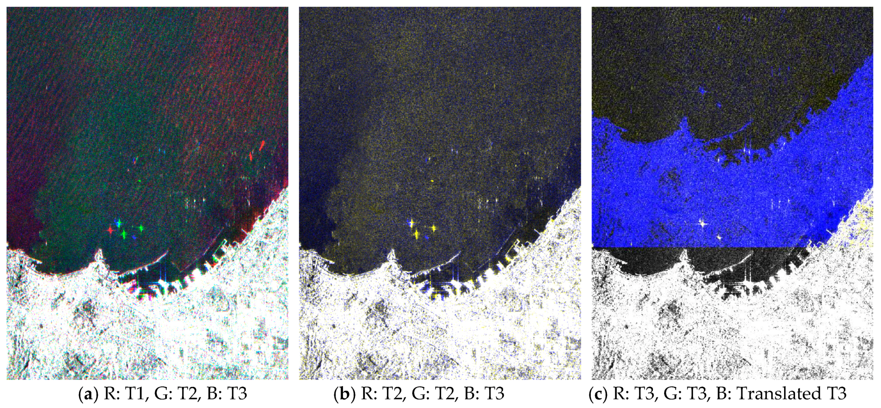
This method is based on temporal consistency of azimuth ambiguities. It also requires same configuration and co-registration. Otherwise the temporal consistence can be lost. In this case, three images are composed as RGB channels directly (one image can be used twice if only two-temporal images available). Thus, azimuth ambiguities and land pixels that are in a good relationship appear in white. Color pixels are associated with low correlation, e.g., moving ship targets in different temporal images.

4.2. Only One Image Available

This method is based on the strong spatial correlation existing between the ambiguity and the related source target. In this case, one image should be used three times in RGB composition. The R and G channels are associated to the original image. The B channel is associated to a copy generated by the original image. The copy is the original image translated in an azimuth ambiguity displacement given by Formula (1) [11]. Similarly, azimuth ambiguities and strong source target pixels that are in good relationship appear in white. Yellow and blue pixels are associated with a low correlation.

In sum, as the consistence of azimuth ambiguities, they always appear in white, whereas other targets on the ocean can appear in color. Thus, they can be used for azimuth ambiguities enhancement and identification.

5. Experimental Results and Discussion

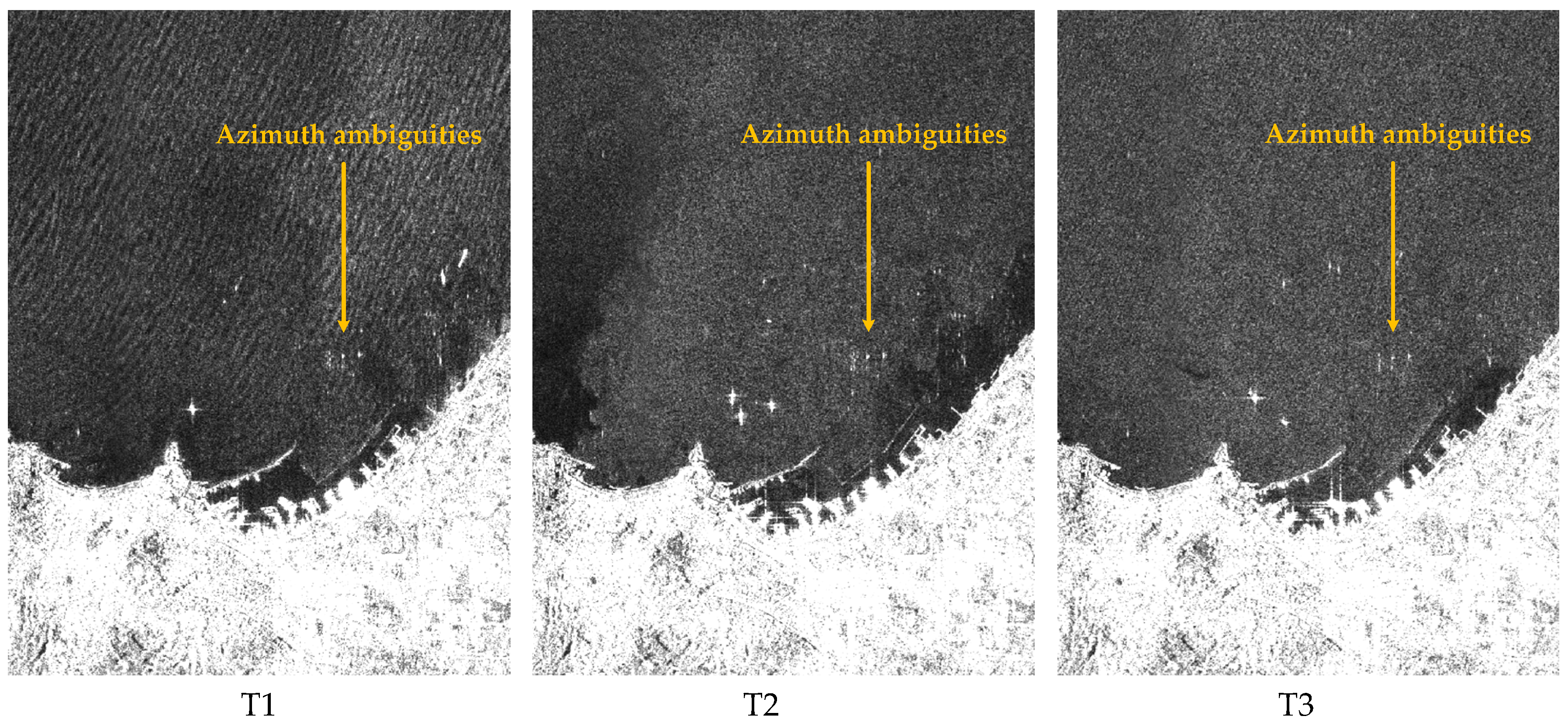
The proposed method is tested on Sentinel-1A IW data first. There are three-temporal images available. The data subsets are presented in Figure 4. They are acquired at 6, 18 February, and 2 March 2017, on Napoli, Italian coast separately. Their polarization modes are VV mode. Azimuth ambiguities are visible in three images, whereas their source targets cannot easily be identified. Thus, it is intractable by using the method by calculating the displacement. QP data is also not available as Sentinel-1 is a dual-polarized system.

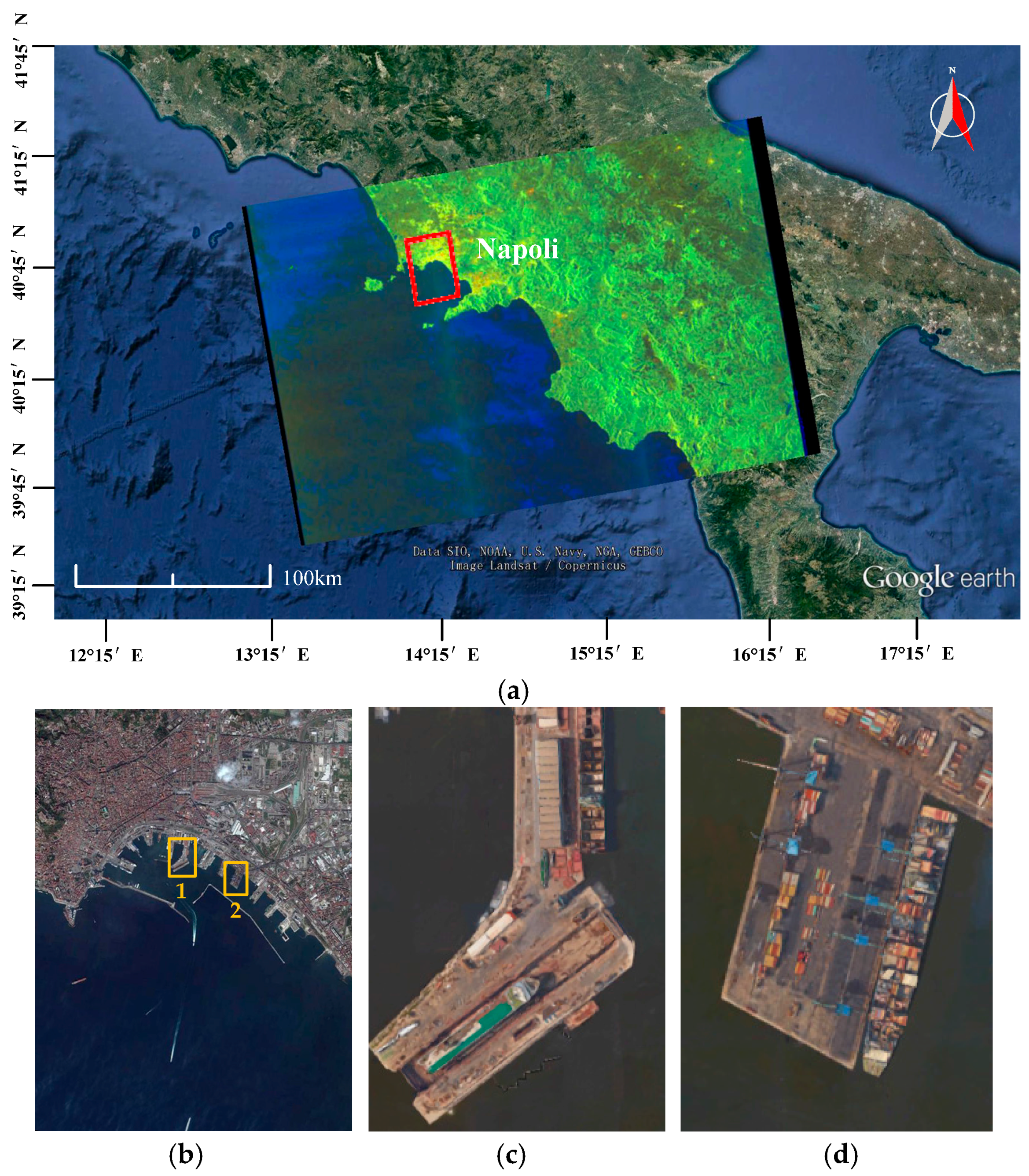
In order to have an overview of the location of the subimage, the optical image (taken from Google Earth) of Napoli is presented in Figure 5a, where the red trectangle indicates the subimage location. Figure 5b is the corresponding optical image of the subimage, where the yellow rectangles 1 and 2 represent the typical ports in Figure 5c,d respectively. The dihedrals of the typical ports in Figure 5c,d can cause strong reflection leading to azimuth ambiguities.

RGB composition results are shown in Figure 6. The results are obtained by different methods presented in Section 4. From the results, it can be seen that white azimuth ambiguities can be recognized more easily than in the original images. The colorful moving ships can also catch one’s eye. Different color represents ships in different period. Compared to the RGB composition methods based on more than two images, the result based on only one image would have a smaller valid size because of the shift operation, as shown in Figure 6c. In this case, strong ship targets also present in white because of its strong spatial correlation between ambiguities. This is distinctive to the method based on more than two images. In sum, azimuth ambiguities always appear in white in all methods. This can help azimuth ambiguity and ship identification in multi-temporal SAR images.

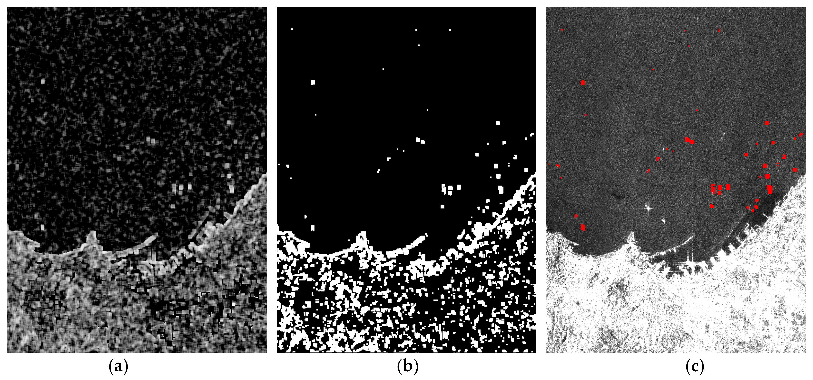
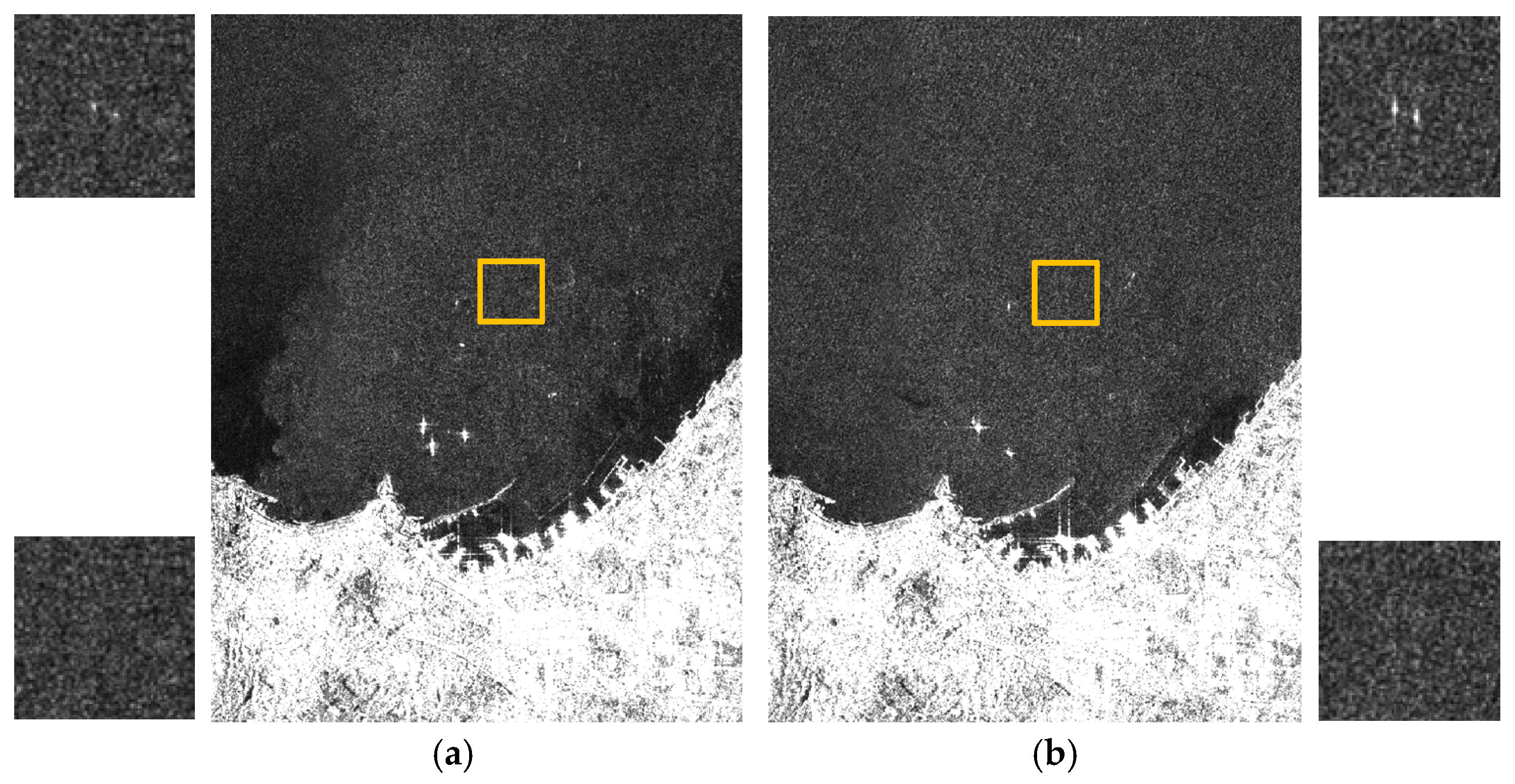
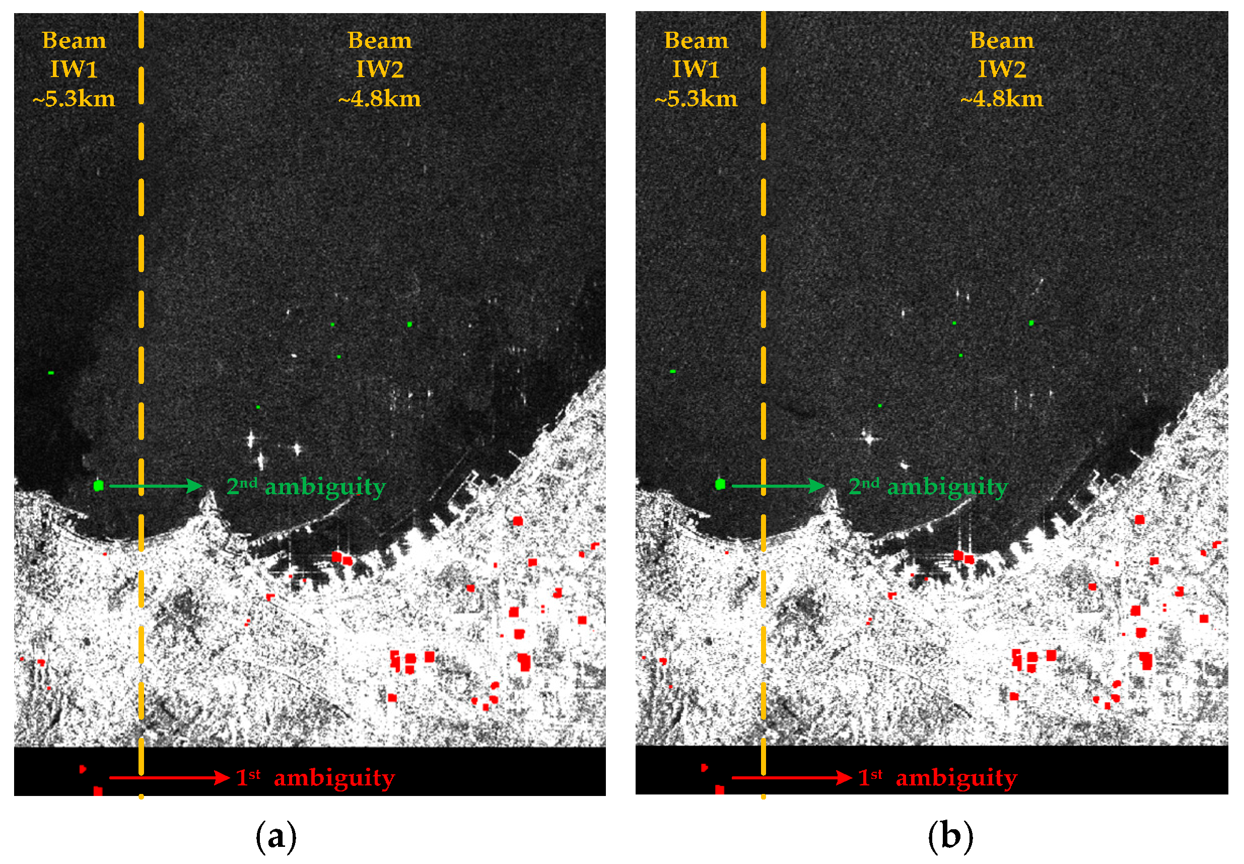
T2 and T3 images are chosen to test the proposed method in this paper. The local window size here is 7. ENL estimated is 7.7. The ambiguity map is shown in Figure 7. Figure 7a is the local correlation coefficient map, Figure 7b is the binarization result, Figure 7c is the T3 ambiguity masks. It can be seen that the proposed method can identify very small azimuth ambiguities. Statistical results show that the azimuth ambiguities with more than 20 pixels can be identified by the proposed method. Some masks may be larger than the actual ambiguities. This is because the local correlation value is not only high for azimuth ambiguities, but also for the surrounding pixels. Figure 8 shows the restored images by the proposed method, which shows a significant enhancement as compared to the original images. The zoomed patches before and after restoration in yellow rectangles are also shown in Figure 8, on the side. Azimuth ambiguities are mitigated effectively. Figure 9 is the inversion to mask strong land sources. The strong land sources are masked as red. Surprisingly, this approach can also distinguish 1st and 2nd order azimuth ambiguities. The red mask on the land can be recognized as 1st order azimuth ambiguities, whereas the green mask on the sea can be recognized as 2nd order azimuth ambiguities or fixed artifacts on the sea. It should be noted that the azimuth displacement in different beams is different. It is ~5.3 km in beam IW1 and 4.8 km in beam IW2 for these images.

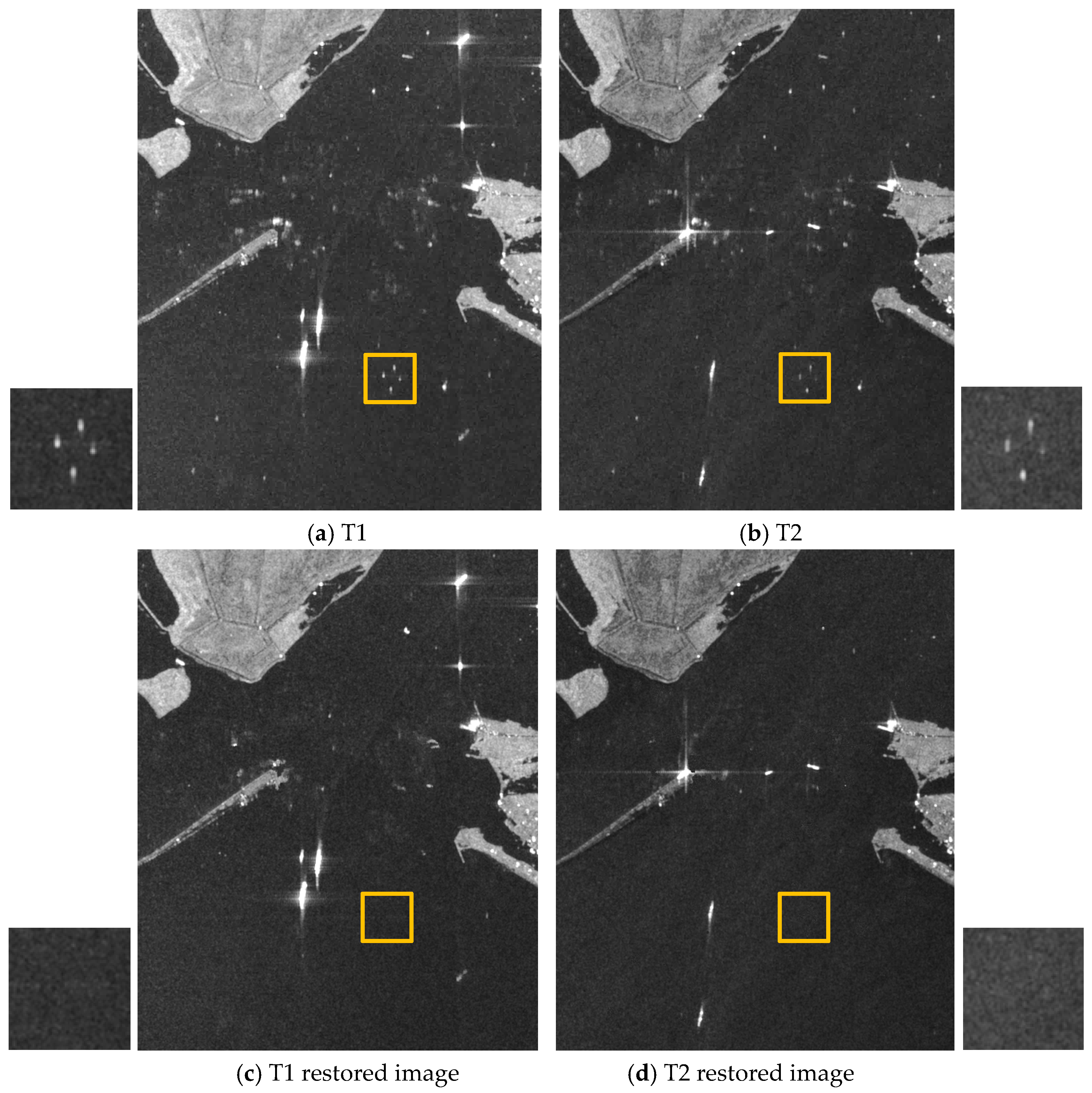
The proposed method is also validated by the Sentinel-1b SM data acquired on Boston, as shown in Figure 10. They are acquired at the 20 March and 1 April 2017, separately. Their polarization modes are HH mode. The zoomed patches before and after restoration in yellow rectangles are also shown in Figure 10. The experimental results show that the proposed method can mitigate most azimuth ambiguities effectively.

The important advantages of the proposed method can be concluded from the experimental results:

(1)

The method by calculating the displacement fails to identify azimuth ambiguities in littoral zones because of the complicated scenes, whereas the proposed method is able to.

(2)

When no QP data is available, the proposed method is a successful candidate for azimuth ambiguities removal in littoral zones.

(3)

The proposed method is a quite tractable method, in which both radiometric correction and speckle filtering are not needed.

(4)

The proposed method only restores azimuth ambiguities areas. There is no change for other areas. Thus, it will not degrade image quality as methods based on SLC products.

(5)

The proposed method can identify very small azimuth ambiguities in detected products, whereas the method by calculating the displacement cannot.

Obviously, though the proposed method is designed to identify azimuth ambiguities, it can also identify other fixed image features, e.g., range ambiguities or fixed artificial structures in multi-temporal images as their temporal consistence. However, small islands in the sea will not be identified by the proposed method because they are removed by the land masking step. We believe that the proposed method would be a practical candidate for ambiguities removal with more multi-temporal images available. The proposed method would be very helpful for ocean monitoring.

The proposed method assumes that the strong land sources are fixed in the period. If the strong land sources changed in the period, the temporal consistence of azimuth ambiguities would decrease. Thus, the proposed method may fail to identify azimuth ambiguities. The method by calculating the azimuth displacement can identify azimuth ambiguities caused by ships on the sea effectively, but fail to identify azimuth ambiguities caused by land sources. Thus, the proposed method can be complementary for it.

6. Conclusions

This paper opens up the possibilities to use multi-temporal SAR data to remove azimuth ambiguities by proposing an azimuth ambiguities removal method in littoral zones based on multi-temporal SAR images. Azimuth ambiguities are identified through an effective technique by the correlation operation of two temporal images. Azimuth ambiguities areas are restored by either a Gaussian distribution or Exemplar-based inpainting techniques based on the homogeneity of sea clutter. Experimental results based on multi-temporal Sentinel-1 IW and SM data validate the effectiveness of the proposed method. It is a successful candidate for azimuth ambiguities removal in littoral zones when no QP product is available. Azimuth ambiguities with more than 20 pixels in IW mode images can be identified by the proposed method. This paper also presents two RGB composition methods for azimuth ambiguities displayed in multi-temporal SAR images. Experimental results show that the RGB composition results can help to enhance azimuth ambiguities for visualization.

Despite the effectiveness of the proposed method, further investigations about how more accurate local correlation needs to be done, which may significantly improve the accuracy of azimuth ambiguities identification.

References

- Curlander, J.C.; McDonoug, R.N. Synthetic Aperture Radar Systems and Signal Processing; John Wiley& Sons: New York, NY, USA, 1991. [Google Scholar]
- Crisp, D.J. The State-of-the-Art in Ship Detection in Synthetic Aperture Radar Imagery; DSTO Information Sciences Laboratory: Edinburgh, Australia, 2004. [Google Scholar]
- Greidanus, H.; Alvarez, M.; Santamaria, C.; Thoorens, F.; Kourti, N.; Argentieri, P. The SUMO ship detector algorithm for satellite radar images. Remote Sens. 2017, 9, 246. [Google Scholar] [CrossRef]
- Brusch, S.; Lehner, S.; Fritz, T.; Soccorsi, M. Ship suveillance with TerraSAR-X. IEEE Trans. Geosci. Remote Sens. 2011, 49, 1092–1103. [Google Scholar] [CrossRef]
- Crisp, D.J. A Ship Detection System for Radarsat-2 Dual-Pol Multi-Look Imagery Implemented in the ADSS. In Proceedings of the 2013 International Conference on Radar (Radar), Adelaide, Australia, 9–12 September 2013; pp. 318–323. [Google Scholar]
- Martorella, M.; Pastina, D.; Berizzi, F.; Lombardo, P. Spaceborne radar imaging of maritime moving targets with the Cosmo-SkyMed SAR system. IEEE J. Sel. Top. Appl. Earth Obs. Remote Sens. 2014, 7, 2797–2810. [Google Scholar] [CrossRef]
- GF-3. Available online: https://www.chinaspaceflight.com/satellite/Gaofen/GF-3/gaofen-3.html (accessed on 1 March 2017).
- Sentinels Scientific Data Hub. Available online: https://scihub.copernicus.eu/ (accessed on 1 September 2014).
- Leng, X.; Ji, K.; Yang, K.; Zou, H. A Bilateral CFAR algorithm for Ship Detection in SAR Images. IEEE Geosci. Remote Sens. Lett. 2015, 12, 1536–1540. [Google Scholar] [CrossRef]
- TerraSAR-X Applications Guide. Extract: Maritime Monitoring: Ship Detection. Airbus Defence and Space Geo-Intelligence Programme Line; Airbus Defence and Space: Toulouse, France, 2015.
- Dellepiane, S.; Martino, M.D.; Toma, M. A data fusion approach for the analysis of azimuth ambiguities. In Proceedings of the 2013 IEEE International Geoscience and Remote Sensing Symposium (IGARSS), Melbourne, Australia, 21–26 July 2013; pp. 4138–4141. [Google Scholar]
- Vespe, M.; Greidanus, H. SAR image quality assessment and indicators for vessel and oil spill detection. IEEE Trans. Geosci. Remote Sens. 2012, 50, 4726–4734. [Google Scholar] [CrossRef]
- Stastny, J.; Hughes, M.; Garcia, D.; Bagnall, B. A novel adaptive synthetic aperture radar ship detection system. In Proceedings of the OCEANS 2011, Waikoloa, HI, USA, 19–22 September 2011; pp. 1–7. [Google Scholar]
- Guarnieri, A.M. Adaptive removal of azimuth ambiguities in SAR images. IEEE Trans. Geosci. Remote Sens. 2005, 43, 625–633. [Google Scholar] [CrossRef]
- Martino, G.D.; Iodice, A.; Riccio, D.; Ruello, G. Filtering of Azimuth Ambiguity in Stripmap Synthetic Aperture Radar Images. IEEE J. Sel. Top. Appl. Earth Obs. Remote Sens. 2014, 7, 3967–3978. [Google Scholar] [CrossRef]
- Liu, C.; Gierull, C.H. A new application for PolSAR imageryin the field of moving target indication/ship detection. IEEE Trans. Geosci. Remote Sens. 2007, 45, 3426–3436. [Google Scholar] [CrossRef]
- Velotto, D.; Soccorsi, M.; Lehner, S. Azimuth ambiguities removal for ship detection using full polarimetric X-Band SAR data. IEEE Trans. Geosci. Remote Sens. 2014, 52, 76–88. [Google Scholar] [CrossRef]
- Wang, C.; Wang, Y.; Liao, M. Removal of azimuth ambiguities and detection of a ship: using polarimetric airborne C-band SAR images. Int. J. Remote Sens. 2012, 33, 3197–3210. [Google Scholar] [CrossRef]
- Greidanus, H.; Santamaria, C. First Analyses of Sentinel-1 Images for Maritime Surveillance. In JRC Science and Policy Reports; Publications Office of the European Union: Luxembourg, 2014. [Google Scholar]
- Leng, X.; Ji, K.; Zhou, S.; Xing, X.; Zou, H. An adaptive ship detection scheme for spaceborne SAR imagery. Sensors 2016, 16, 1345. [Google Scholar] [CrossRef] [PubMed]
- Wessel, P. GSHHG—A Global Self-Consistent, Hierarchical, High-Resolution Geography Database. Available online: http://www.soest.hawaii.edu/pwessel/gshhg (accessed on 1 September 2014).
- Baselice, F.; Ferraioli, G. Unsupervised coastal line extraction from SAR images. IEEE Geosci. Remote Sens. Lett. 2013, 10, 1350–1354. [Google Scholar] [CrossRef]
- Niedermeier, A.; Romaneessen, E.; Lehner, S. Detection of coastlines in SAR images using wavelet methods. IEEE Trans. Geosci. Remote Sens. 2000, 38, 2270–2281. [Google Scholar] [CrossRef]
- Kapur, J.N.; Sahoo, P.K.; Wong, A.K.C. A new method for gray-level picture thresholding using the entropy of the histogram. Comput. Vis. Graph. Image Process. 1985, 29, 273–285. [Google Scholar] [CrossRef]
- Otsu, N. A Threshold Selection Method from Gray-Level Histogram. IEEE Trans. Syst. Man Cybern. 1979, 9, 62–66. [Google Scholar] [CrossRef]
- Sahoo, P.K.; Soltani, S.; Wong, A.K.C. A survey of thresholding techniques. Comput. Vis. Graph. Image Process. 1988, 41, 233–260. [Google Scholar] [CrossRef]
- Criminisi, A.; Perez, P.; Toyama, K. Region filling and object removal by exemplar-based image inpainting. IEEE Trans. Image Process. 2004, 13, 1200–1212. [Google Scholar] [CrossRef] [PubMed]
- Cossu, R.; Schoepfer, E.; Bally, P.; Fusco, L. Near real-time SAR-based processing to support flood monitoring. J. Real-Time Image Process. 2009, 4, 205–218. [Google Scholar] [CrossRef]
- Dellepiane, S.G.; Angiati, E. A New Method for Cross-Normalization and Multitemporal Visualization of SAR Images for the Detection of Flooded Areas. IEEE Trans. Geosci. Remote Sens. 2012, 50, 2765–2779. [Google Scholar] [CrossRef]
Figure 1.
Illustration of azimuth ambiguity formation in SAR images, targets A and B have equal Doppler histories due to aliasing [20].
Figure 2.
Examples of azimuth ambiguities in current synthetic aperture radar (SAR) imagery, (a) TerraSAR-X StripMap image, azimuth displacement is ~4.4 km (b) COSMOS-SkyMed StripMap image, azimuth displacement is ~4.4 km (c) RADARSAT-2 Standard mode image, azimuth displacement is ~5.2 km (d) Sentinel-1 IW image, azimuth displacement is ~4.7 km (beam IW2).
Figure 3.
The flowchart of the proposed method. It includes co-registration, local correlation, binarization, masking, and restoration steps. The idea underlying the proposed method is that sea surface is dynamic whereas azimuth ambiguities caused by land-based sources are constant. It is designed to remove azimuth ambiguities caused by fixed land-based sources.
Figure 4.
The Sentinel-1A multi-temporal dataset. The similar clusters of dots in T1, T2 and T3 at the same location are prominent azimuth ambiguities from the strong source targets on land. T1: S1A_IW_GRDH_1SDV_20170206T165649_20170206T165714_015166_018D05_8064; T2: S1A_IW_GRDH_1SDV_20170218T165649_20170218T165714_015341_01927E_D691; T3: S1A_IW_GRDH_1SDV_20170302T165648_20170302T165713_015516_0197CF_75D4.
Figure 5.
Google Earth image indicating the Sentinel-1A images. The red rectangle in (a) indicates the subimage location in Figure 4, (b) is the corresponding optical image of the subimage, yellow rectangles 1 and 2 represent the typical ports (c) and (d) which can cause azimuth ambiguities respectively.
Figure 6.
RGB composition results of the Sentinel-1A multi-temporal data. Azimuth ambiguities appearing white in (a–c) can be recognized more easily than in the original images. A ship target in (b) seems to be white as there is a blue target near it. (c) has a smaller valid size because of the shift operation.
Figure 7.
Azimuth ambiguity mask, (a) local correlation coefficient map, (b) binarization result, (c) T3 ambiguity mask.
Figure 8.
Restored images, (a) T2 restored image, (b) T3 restored image. The zoomed patches before and after restoration in yellow rectangles are shown on the side.
Figure 9.
Inversion to mask strong land sources, (a) T2 image, (b) T3 image. The strong land sources are masked as red. Note that the azimuth displacement in different beams is different, ~5.3 km in beam IW1 and 4.8 km in beam IW2. Red masks on the land can be recognized as 1st order azimuth ambiguities whereas green masks can be recognized as 2nd order azimuth ambiguities or fixed artifacts on the sea.
Figure 10.
Azimuth ambiguities removal results. (a,b) Original Sentinel 1-b images, (c,d) Restored Sentinel-1b images. The zoomed patches before and after restoration in yellow rectangles are shown on the side. T1: S1B_S6_GRDH_1SDH_20170320T002541_20170320T002604_004785_0085BB_9204; T2: S1B_S6_GRDH_1SDH_20170401T002541_20170401T002605_004960_008AC4_D8E2.
© 2017 by the authors. Licensee MDPI, Basel, Switzerland. This article is an open access article distributed under the terms and conditions of the Creative Commons Attribution (CC BY) license (http://creativecommons.org/licenses/by/4.0/).
Share and Cite
MDPI and ACS Style
Leng, X.; Ji, K.; Zhou, S.; Zou, H. Azimuth Ambiguities Removal in Littoral Zones Based on Multi-Temporal SAR Images. Remote Sens. 2017, 9, 866. https://0-doi-org.brum.beds.ac.uk/10.3390/rs9080866
AMA Style
Leng X, Ji K, Zhou S, Zou H. Azimuth Ambiguities Removal in Littoral Zones Based on Multi-Temporal SAR Images. Remote Sensing. 2017; 9(8):866. https://0-doi-org.brum.beds.ac.uk/10.3390/rs9080866
Chicago/Turabian StyleLeng, Xiangguang, Kefeng Ji, Shilin Zhou, and Huanxin Zou. 2017. "Azimuth Ambiguities Removal in Littoral Zones Based on Multi-Temporal SAR Images" Remote Sensing 9, no. 8: 866. https://0-doi-org.brum.beds.ac.uk/10.3390/rs9080866
Note that from the first issue of 2016, this journal uses article numbers instead of page numbers. See further details here.