Sparse Weighted Constrained Energy Minimization for Accurate Remote Sensing Image Target Detection

Lab of Video and Image Processing Systems, School of Electronic Engineering, Xidian University, Xi’an 710071, China
*
Author to whom correspondence should be addressed.
Remote Sens. 2017, 9(11), 1190; https://0-doi-org.brum.beds.ac.uk/10.3390/rs9111190
Submission received: 9 October 2017
/
Revised: 15 November 2017
/
Accepted: 15 November 2017
/
Published: 20 November 2017
(This article belongs to the Section Remote Sensing Image Processing)
Abstract
:Target detection is an important task for remote sensing images, while it is still difficult to obtain satisfied performance when some images possess complex and confusion spectrum information, for example, the high similarity between target and background spectrum under some circumstance. Traditional detectors always detect target without any preprocessing procedure, which can increase the difference between target spectrum and background spectrum. Therefore, these methods could not discriminate the target from complex or similar background effectively. In this paper, sparse representation was introduced to weight each pixel for further increasing the difference between target and background spectrum. According to sparse reconstruction error matrix of pixels on images, adaptive weights will be assigned to each pixel for improving the difference between target and background spectrum. Furthermore, the sparse weighted-based constrained energy minimization method only needs to construct target dictionary, which is easier to acquire. Then, according to more distinct spectrum characteristic, the detectors can distinguish target from background more effectively and efficiency. Comparing with state-of-the-arts of target detection on remote sensing images, the proposed method can obtain more sensitive and accurate detection performance. In addition, the method is more robust to complex background than the other methods.
1. Introduction
With the rapid development of remote sensing technology, the spatial resolution, spectral resolution and time resolution of remote sensing image have greatly improved, which facilitates a wide range of applications [1,2,3,4]. Remote sensing image contains abundant information, of which the processing and analyzing can help people in not only military but also civilian applications, such as disaster control, land planning, urban monitoring, traffic planning, target tracking, etc. [5,6,7]. For all these applications, target detection is the necessary and key step. The targets are usually large objects, such as aircraft, ship, building, etc., which can provide more valuable object for further analyzing. However, the object detection is usually human, animal and other small objects, and the target is not limited to one specific category. Research of fast identification and precise interpretation on particular target has very important strategic significance [8,9].
Therefore, target detection has received considerable attention and has always been the research hotspot in remote sensing in the past decades [10,11,12,13]. A number of target detection algorithms emerged along with the development of remote sensing. Most of these algorithms tend to suppress background information and highlight target to enhance the target itself, e.g., adaptive coherence estimator (ACE) [9,14], match filter (MF) [14], adaptive match filter (AMF) [9,15,16,17,18], spectral angle mapper (SAM) [17], independent component analysis (ICA) [18], and constrained energy minimization (CEM) [19,20]. Stephanie et al. pointed out that ACE is known to be the generalized likelihood ratio test (GLRT) in partially homogeneous environments, when the covariance matrix of the secondary data is proportional to the covariance matrix of the vector under test [21]. Similar to ACE, MF and AMF, which consider target detection as the problem of hypothesis testing, they often employ the local background statistics. Actually, target and background usually follow different probability models, and the generalized likelihood ratio test (GLRT) is used to detect target. The SAM algorithm treats both spectra of target and background as vector, and then calculates the spectral angle between them. It is an automated method that can directly compare image spectra to a known spectrum (usually measured by a spectrometer in the lab or field) or an end member. This algorithm is insensitive to illumination, because the SAM uses vector direction instead of vector length. William et al. proposed a CEM algorithm to map the ferruginous sediments. They pointed out that CEM, which is conducted pixel-by-pixel, could maximize the response of target signature and meanwhile suppress the response of undesired background signatures, so that the target and background can be discriminated easier [19]. Actually, CEM constructs a finite-impulse response (FIR) filter, which minimizes the output energy under constraint that the filter’s response to spectral signature of target is unity [22]. Although these methods have achieved impressive performance and been widely used, more and more complicated background will make the detection accuracy declined unexpectedly. Therefore, many improved algorithms are developed for further improving the detection performance under different situation. Shuo et al. proposed both sparse CEM and sparse ACE algorithms using the -norm regularization term to restrict the output to be sparse [23]. They hope that the output of detection is sparse, since target of interests usually occupy a few pixels (or even subpixels) in real remote sensing images. Geng et al. proposed a novel ACEM, and they proved that ACEM is mathematically equivalent to MF (matched filter). They concluded that the classical MF is always superior to the CEM operator [24]. Zheng et al. proposed a new hierarchical method called hierarchical CEM (hCEM) to suppress the backgrounds while preserve the target spectra with the purpose of boosting the performance of traditional target detector [25]. In practice applications, target spectra are always diverse, and most existing methods perform a hard constraint on the target spectrum, which will bring more difficulties to detect target accurately. Consider the situation, Shuo et al. proposed a target detection algorithm by employing an inequality constraint, which is more robust to spectral diversity, as they made a soft constraint on target spectrum to cover more styles [26]. Geng et al. also proposed a Clever eye (CE) [27] method that can automatically search the best data origin to move the data cloud to, and find the optimal direction to project the data on. Accordingly, CE can always obtain lower output energy than CEM and MF. Wang et al. proposed a two-time detection scheme by employing principal component CEM and matrix taper CEM simultaneously [28].
The methods described above only concerned one kind of spectrum, which is obviously not consistent with actual situation. Most remote sensing images, which include multiple targets or target itself, possess multiple spectrum characteristics. To detect all kinds of targets in a single image simultaneously, Chein et al. developed several multiple target detection approaches, e.g., Multiple-target CEM (MTCEM), Sum CEM (SCEM), and Winner-Take-All CEM (WTACEM) [29]. These methods utilized only the known target spectral information but not the background spectral information. Considering both target and background spectrum as a priori information, several detection methods utilized both target and background spectral information were proposed to obtain better performance. Orthogonal subspace projection (OSP), based on linear mixed model [30], aimed at eliminating the background signatures. Matched subspace detector (MSD) assumes both target and background spectrum obey the Gaussian distribution [31], with the same-scaled identity covariance matrix and differ only in their means [32]. A novel Symmetric Sparse Representation (SSR) method has been presented to solve the band selection problem in hyperspectral imagery (HSI) classification by Sun et al. [33]. The above methods analyzed both target and background spectrum, however, they did not do anything to further increase the difference between target and background spectral information, which probably lead to the false positive rate unexpectedly increasing as the variability of spectral information.
In the state-of-the-arts, the methods based on sparse representation still report satisfactory performance in recent years, especially in classification and target detection [34,35,36,37,38]. These methods usually need to construct two dictionaries, the target dictionary and union dictionary that contains both target and background. Then, they use these two dictionaries to sparsely represent the spectral information and get the sparse coefficient to obtain reconstruction error. The quality of the dictionaries plays an important role in the detection performance, especially the background dictionary, which is always difficult to obtain. An effective way to construct the dictionary is to build a dual concentric window [37], which is an adaptive local dictionary method. It needs to set the window sizes in advance, however, there is no specific method to choose the appropriate size. For the purpose of reducing the impact of target pollution, another method based on learning has been proposed. Although there are many algorithms about constructing dictionary, how to construct an effective dictionary is still a difficult problem. The target spectral is always more intuitive with small amount, and the background spectral is always complicated and large. Thus, the target dictionary is easier to get while the background dictionary is more difficult to obtain.
To solve the above problems, in this paper, a novel sparse weighted-based constrained energy minimization (SWCEM) target detection method is proposed. Based on the constrained energy minimization (CEM) algorithm, the proposed method first introduced the effective sparse representation to weight the spectral characteristics with sparse information, which can effectively increase the difference between target and background spectrum. Since the spectrums are always diverse, target may possess similar spectrum characteristics with background. It will make the target detection more difficult. Unlike the CEM algorithm, which only uses the spectral information of original target and background pixels, the proposed SWCEM method adaptively assigned weights to each pixel according to their reconstruction error matrix of sparse representation. It adaptively assigned greater weight to target pixel, and smaller weight to background pixel, which can effectively increase the difference between target pixels and background pixels. Then, comparing with the exist sparse representation based methods, the SWCEM algorithm only needs to construct target dictionary, and calculate the similarity between spectrums of pixels and recovery of residual. Since the sparse weighted procedure could improve the identification degree between target and background, we do not need to establish the background dictionary that is hard to get. It makes the similarity measure more scientific and accurate.
The remainder of this paper is organized as follows: Section 2 introduces the proposed sparse weighted CEM (SWCEM) method in detail. Section 3 describes the dataset we employed and illustrates the performance of the proposed method. Then, Section 4 analyzes and discusses the experimental results. Finally, conclusions are exhibited in Section 5.
2. The Proposed Method
In this section, the original CEM and sparse representation will be introduced firstly, and then the proposed SWCEM algorithm will be described in detail.
2.1. CEM Algorithm
Assume that is the spectral information of remote sensing image, N is the number of pixels, each pixel is a L-dimensional vector, L is the number of band, and , is an matrix. Suppose d is the target spectrum as a priori information, the main idea of CEM is to design a linear FIR (Finite Impulse Response) filter that minimizes the average energy output under the following constraint:
where is filter coefficient, which is an L-dimensional vector. Suppose that the output of the above filter corresponding to input is :
the average output energy from all input can be calculated by,
where represents the autocorrelation matrix of remote sensing image , and is the output of each pixel. CEM algorithm can be expressed as the following linear constraint optimization problem.
This is an equal constraint optimization problem, which can be solved by Lagrange multiplier [35]. The optimized solution of Equation (4) is:
so the output of CEM filter is:
The CEM algorithm can detect target of interest, while minimizing the output energy caused by other unknown signals. The larger the pixel output energy, the greater the probability of the target is. Otherwise, the pixel has lower probability as target.
2.2. Sparse Representation Algorithm
In sparse representation, the target dictionary can be represented as , whose columns are , and the background dictionary can be represented as , where and are the numbers of atoms in target and background dictionary, respectively. The classical sparse representation based classification relies on the underlying assumption that a test sample can be linearly represented by a small number of training samples class [34]. Thus, for a background pixel , it can be better represented as a linear combination of atoms in background dictionary as follows:
where α is a sparse vector whose entries are abundances of corresponding atoms in the background dictionary [39,40].
Similarly, if is a target pixel, it can be better represented as a linear combination of the atoms union in background dictionary and the target dictionary as follows:
where is the union dictionary contains both the background dictionary and the target dictionary , β is the sparse coefficient.
Given a pixel , it can be represented by background dictionary and union dictionary , respectively. The sparse vector can be recovered by solving:
where and are given upper bound on the sparsity level, and the sparsity level parameters adopt the same values as in Zhang et al. [34]. The aforementioned problem has been solved by the orthogonal matching pursuit (OMP) algorithm [41]. Then, the test pixel can be reconstructed by these two dictionaries as follows:
The reconstructed spectrum can be determined by comparing the reconstruction error of the mean squared error under two hypotheses [42,43,44]. The residuals of recovery [45] can be obtained as:
where and represent the recovered sparse coefficients corresponding to the background and target dictionaries, respectively.
Finally, we can get the detector of sparse representation algorithm:
If is a background pixel, the values of and are similar, then will be a small value. If is a target pixel, the value of will be much larger than , and will be a bigger value. Through the above analysis, the larger the value of , the greater the probability of target for the pixel is.
2.3. SWCEM Algorithm
Remote sensing images contain very complex information, most of the complex information come from background and we are not so interested in it. It is difficult to figure out what the background information exactly is, while target information is relatively easier to get. The SWCEM algorithm only concerns about the target information. It only needs to construct the target dictionary, rather than constructing both target and background dictionary, which is more convenient and easier to implement.
Suppose that is the target dictionary containing all possible target spectral information. A remote sensing image with N pixels and L bands can be represented as an matrix , where , . The pixel can be represented by the target dictionary D, like the sparse representation mentioned above:
The sparse vector can be recovered by solving:
where is given upper bound on the sparsity level, the OMP algorithm is used to solve the problem [41]. Then, we can reconstruct the pixel and get the residual of recovery:
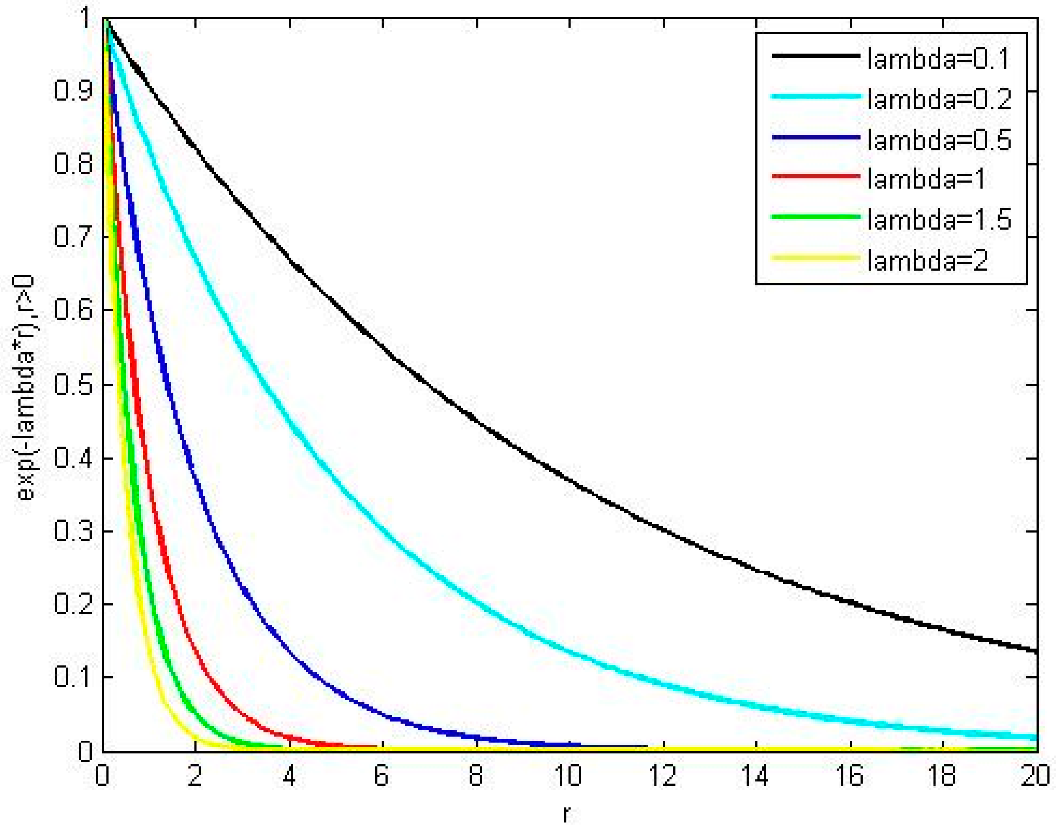
The recovery residual characterizes the similarity between pixel and target. However, some target pixels possess so similar spectral information with background pixels that the original CEM often reports weak ability to distinguish them and does not obtain satisfied detection results. To further increase the discriminated power between target and background, an adaptive weight is assigned to each pixel based on the recovery residual. According to sparse representation, bigger recovery residual always announces the higher probability that the pixel belongs to the background. Then, we will assign a smaller weight to these pixels to suppress their contributions. Similarly, we will give a bigger weight to the pixel with smaller recovery residual, which possess higher probability to be target. After that, the target spectrum will present more distinct characteristic compared with background. We employ the exponential style, and design a novel weight function to achieve this purpose. The proposed weight function is expressed as below and also shown in Figure 1.
In the same way, we assign the adaptive weight to each pixel to get a new weighted remote sensing data, which can be represented by matrix as follows:
where , . Based on the original CEM, we can get the autocorrelation matrix of new remote sensing data :
so the optimization problem in Equation (4) can be re-expressed as follows:
where w and d express the same meaning as the original CEM, and the solution of Equation (20) can also be obtained by Lagrange multiplier method [40]:
Then, the final output of the SWCEM is:
Therefore, we effectively increase the difference between target and background pixels according to their essential characteristics, and then the detector can distinguish the target from background more easily. It produces a large output value to target pixels, while a small value to background pixels. Therefore, the target will be separated from background clearly. The outline of the proposed SWCEM algorithm can be described in Algorithm 1.
| Algorithm 1 SWCEM Algorithm | |
| Input: | |
| spectral matrix , target spectrum , target dictionary , parameter λ, sparse level δ. | |
| Sparse weighted: | |
| 1. Target dictionary : | |
| 2. Recovery residual and the weight | |
| 3. | |
| Constrained Energy Minimization: | |
| 4. Get the autocorrelation matrix: | |
| 5. | |
| 6. Solve the optimization problem: | |
| Output: | |
| 7. final output: | |
3. Results
In this paper, four remote sensing datasets are used to evaluate the effectiveness of proposed SWCEM algorithm. These datasets all possess their own distinctive characteristics, i.e., source of the data, target size, environment around the target, and spatial resolution. The proposed SWCEM algorithm just adopted two parameters, the λ and sparse level . Since there is no specific method to set the parameter value automatically, we set them manually according to experience. Generally, λ ranges 0~10, with the sparse level ranges 1~5. We also compare the proposed method with exist advanced target detection algorithms, such as CEM, SAM, hCEM, CE, and MPCEM. The CEM and SAM are classic target detection algorithms, and CE, hCEM, and MPCEM are latest improved versions of CEM. The proposed method employs the parameters setting in hCEM, and the procedure with results are presented and discussed as follows.
3.1. Experiment on the First Dataset
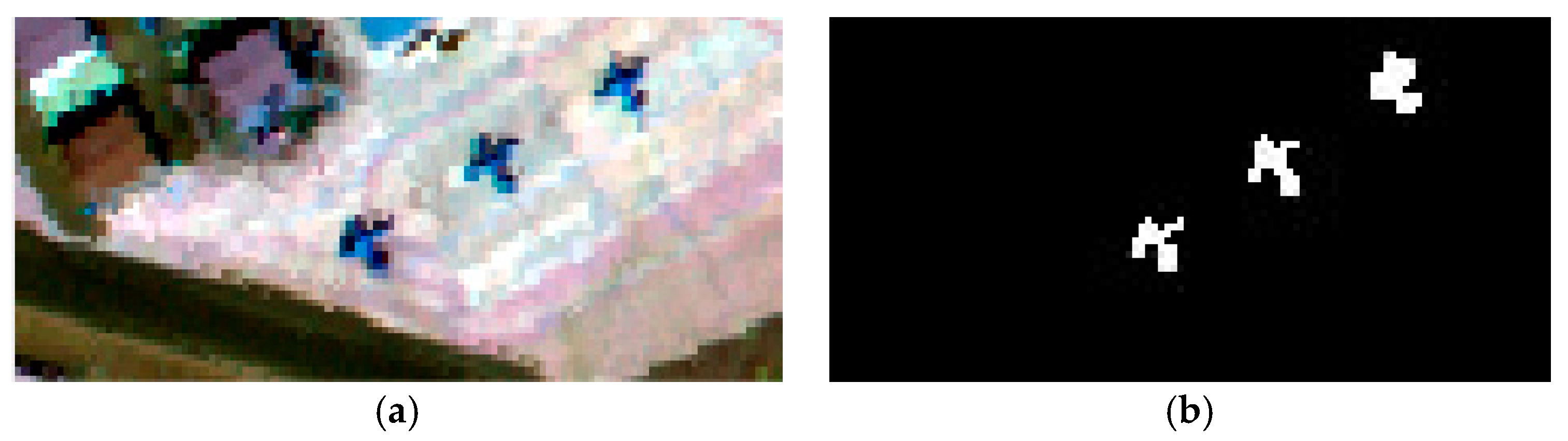
The first dataset is acquired from SPOT6 satellite, which is provided by Digital Globe Incorporated, the acquisition time is November 2012. It is a scene of Xianyang Airport in Shanxi Province, China. It has four spectral bands that include blue band (0.455 to 0.525), green band (0.530 to 0.590), red band (0.625 to 0.695) and near infrared band (0.760 to 0.890). The spatial resolution is 2 for each band. Most of the scene is building area, and only a small part of it is the airport runway. We select two scenes from the data to conduct the experiment, and regard the airplane as the target to be detected. The first scene is pixels, and the plane stays on the runway; the second scene is pixels, with plane stays down the parking shed. These two scenes have different interference information: the first is impacted by lawn pool; and the second is parking shed with a spectrum similar to the plane. The false color image and reference data of the first scene are presented in Figure 2, while the false color image and the reference data of the second scene are presented in Figure 3.
The reference data are the ground truth of targets, which is marked by experts. Usually, the spectral information of target can be obtained from the spectral library, but it is not available here. Therefore, we averaged part of the marked target spectrum as the target spectrum . In Figure 2 and Figure 3, we can see that the spectrum of wings and back on the plane are obviously different, so the target spectrum should cover both the spectra of wings and back on plane. Dictionary constructed by target spectrum contains all possible target spectra, so the final target dictionary has 276 atoms consists of target spectrum of these two scenes. The detection results of these data are presented in Figure 4 and Figure 5.
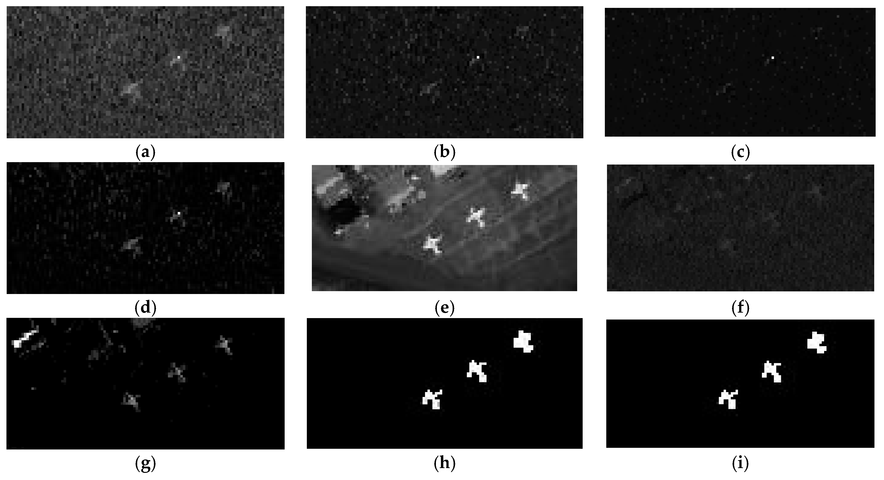
In the experiment, the hCEM converged in the third layer. The first row in Figure 4 and Figure 5 shows the detection results of hCEM on each layer during iteration. The second row shows the detection results of CEM, SAM and CE, respectively. The third row shows the detection results of latest MPCEM, the proposed SWCEM, and the ground truth, respectively. We can find that hCEM indeed gradually improves the detection performance when layer increasing. While, if the original detection was inaccurate, it will result in more inaccurate results on following layers. The spectrum of lawn pool in first scene and spectrum of parking shed in second scene are all similar to the target spectrum, so the hCEM, CEM, SAM, CE, and MPCEM all failed to suppress the complex background. For the proposed SWCEM algorithm, the small weight is assigned to background pixel and a larger weight is set to target pixel according to the adaptively sparse weighting. In this case, the spectrum characteristics of target and background will present great difference, and the method could effectively suppress the background while highlight the target. Then, obviously, we can see from the detection results that the proposed SWCEM algorithm could obtain more clean background. We also find that SWCEM only detected the plane back while missed the plane wings, this is because the target spectrum d was selected from the plane back only. However, there is a big difference between the spectrum of plane wing and plane back, so the SWCEM suppressed the plane wing as background. On the other hand, the results also show that the proposed method can well suppress the spectrum that is different from the target spectrum, and obtain more clean detection results.
3.2. Experiment on the Second Dataset
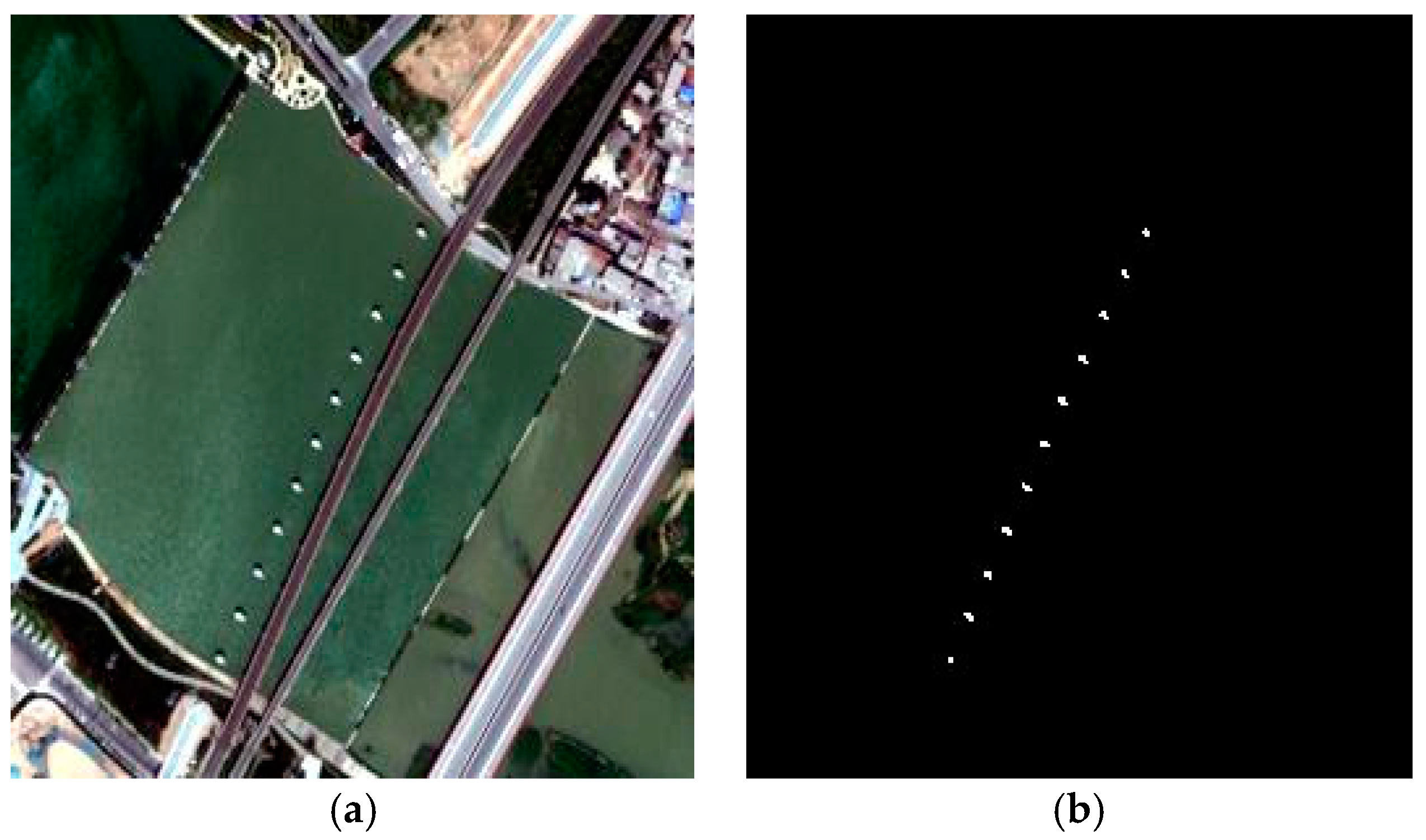
We also test the proposed SWCEM algorithm on the second dataset, which is acquired from SPOT6. The data were captured in Chanba, Xi’an City, Shanxi Province, China, in 2011. It has four spectral bands that include blue band (0.455 to 0.525 ), green band (0.530 to 0.590 ), red band (0.625 to 0.695 ), and near infrared band (0.760 to 0.890 ). The spatial resolution is 2 m for each band. We selected one scene from the data, which has 258×261 pixels, containing a large area of water. The target we selected here is bridge pier surrounded by water. In this scene, targets account for very few pixels, and we should precisely separate the target from water. The false color image and reference data are presented in Figure 6. We randomly selected one pixel from the target spectrum as target spectrum , and we constructed the target dictionary with all the target spectrum. The detection results of these data are presented in Figure 7.
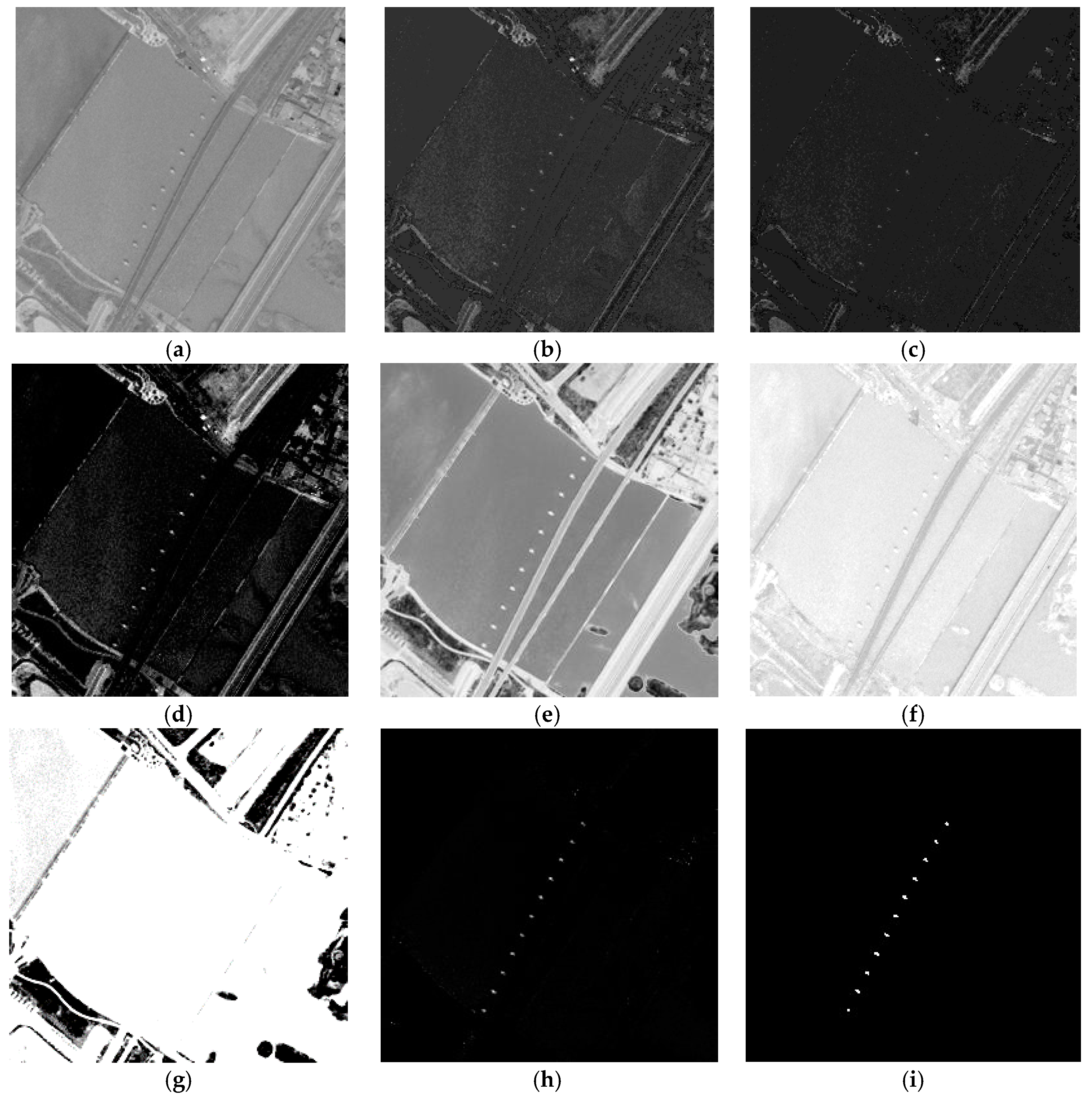
The first row in Figure 7 also shows the detection results of hCEM from the first to third iterate layer. The second row shows the detection results of CEM, SAM and CE. The third row in Figure 7 presents the detection results of MPCEM, the proposed SWCEM and the reference data. The hCEM algorithm converged on the twelfth layer in this test, but the detection results seem not improves anymore from the third layer. Thus, we only show the results about first three layers. We can find that without background suppression, the detection results still reserved many backgrounds, which makes the results more confused for understanding. By contrast, the proposed SWCEM algorithm produces relatively clean and better detection result. This should be attributed to the adaptively weighting procedure, which suppress the undesired background spectrum and simultaneously ensure the target spectrum more significant.
3.3. Experiment on the Third Dataset
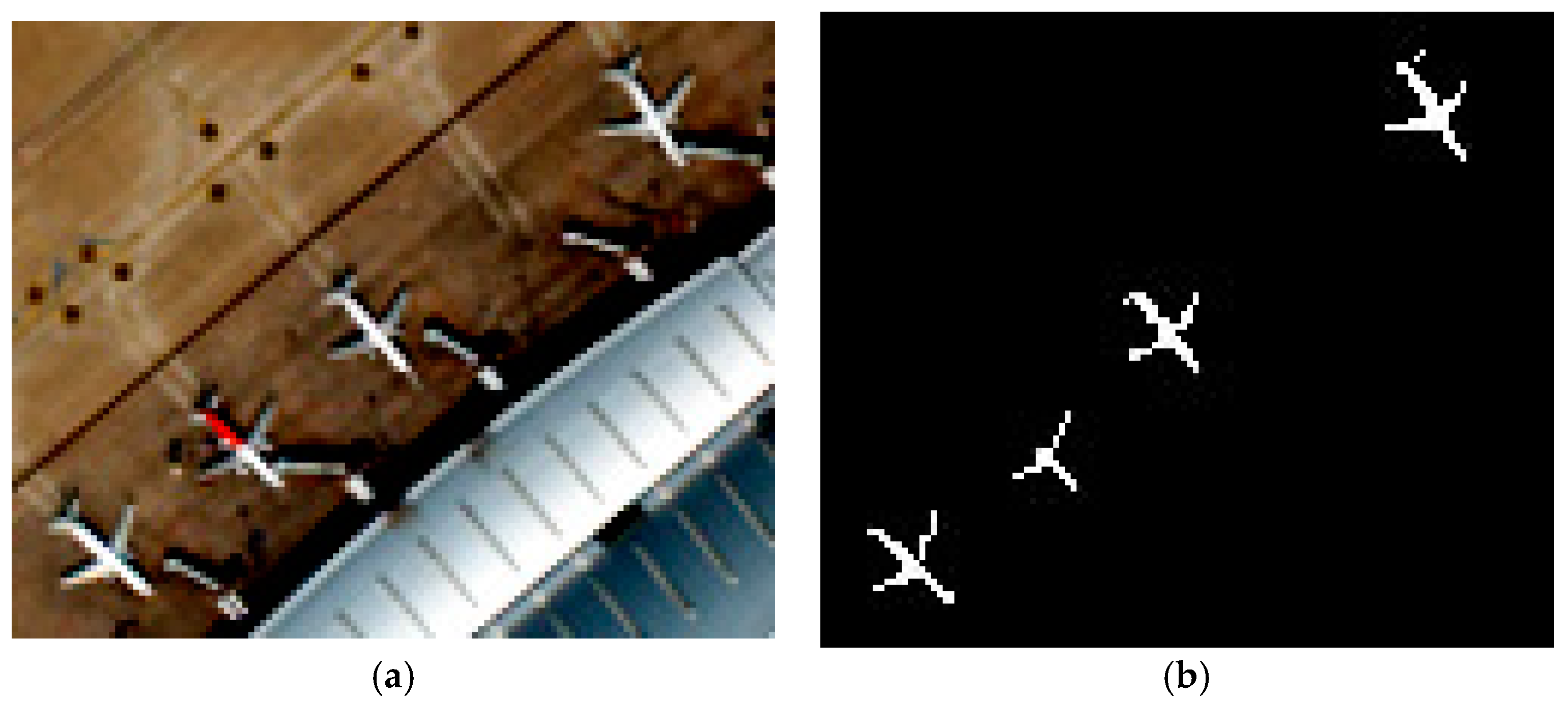
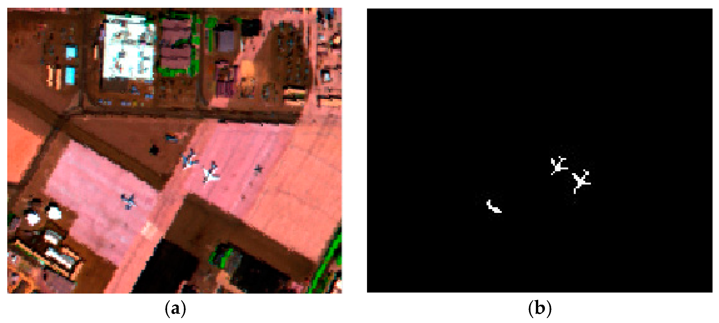
Then, to further evaluate the proposed method, we test the SWCEM algorithm on another kind of dataset, a famous hyperspectral dataset. It was collected by the Airborne Visible/Infrared Imaging Spectrometer (AVIRIS), and presents the scene of the airport in San Diego, CA, USA. The data have 224 spectral channels in wavelengths ranging from 370 nm to 2510 nm. After removing the bands that correspond to water absorption regions, low SNR, and bad bands (1–6, 33–35, 97, 107–113, 153–166, and 221–224), the remaining 189 available bands are retained in the experiments. The spatial resolution is 3.5 m for each band. From this hyperspectral dataset, we selected one scene to test. The scene is 150 × 182 pixels, which can be seen in Figure 8. The pseudo color image of the hyperspectral and the reference data are presented in Figure 8. The reference data are also the ground truth of targets marked by experts. In Figure 8, we can see that there are three planes in the scene, which are selected as the target to be detected. The target spectrum and dictionary are selected and constructed similarly with the former tests, and the detection results are presented in Figure 9.
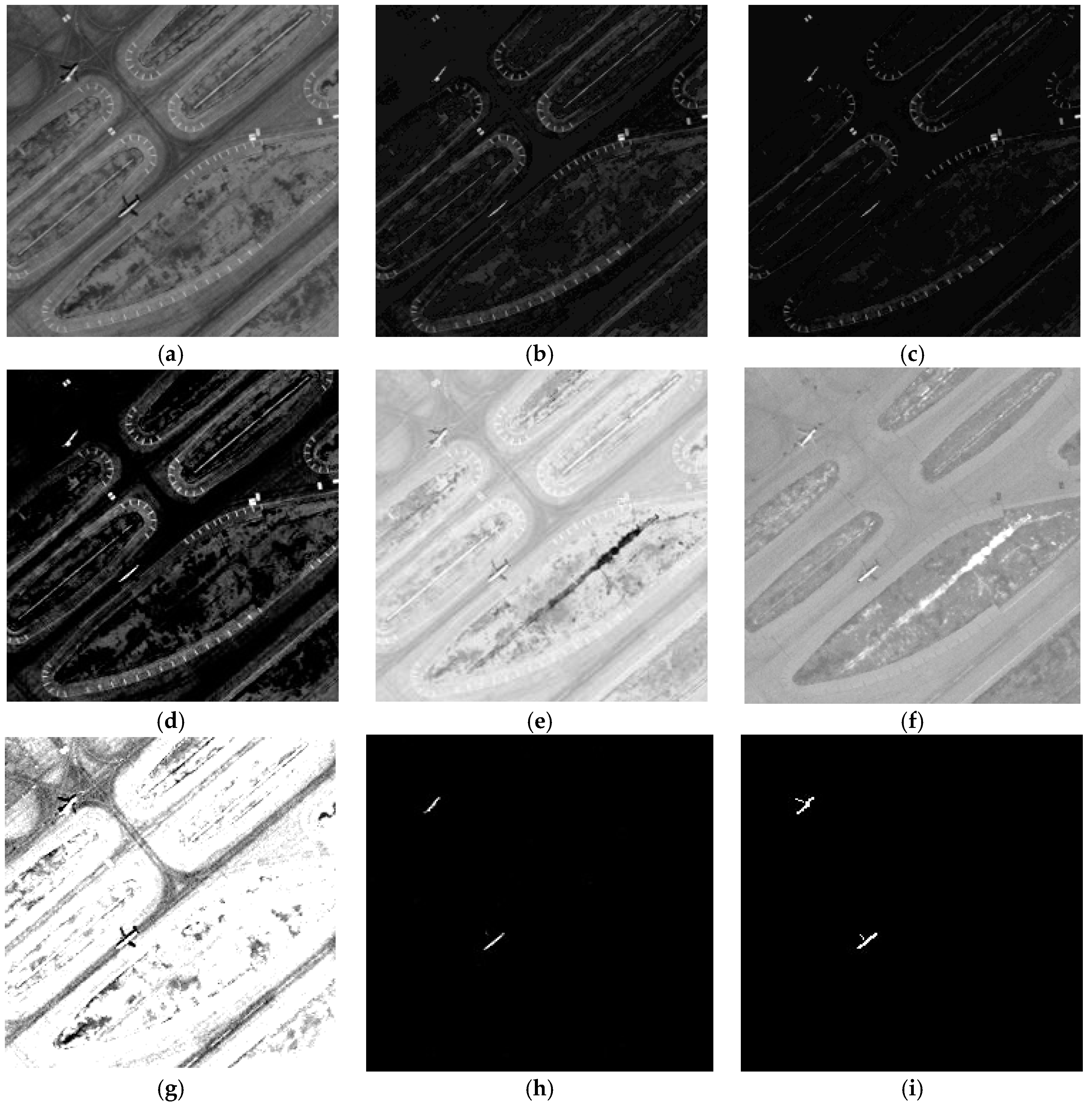
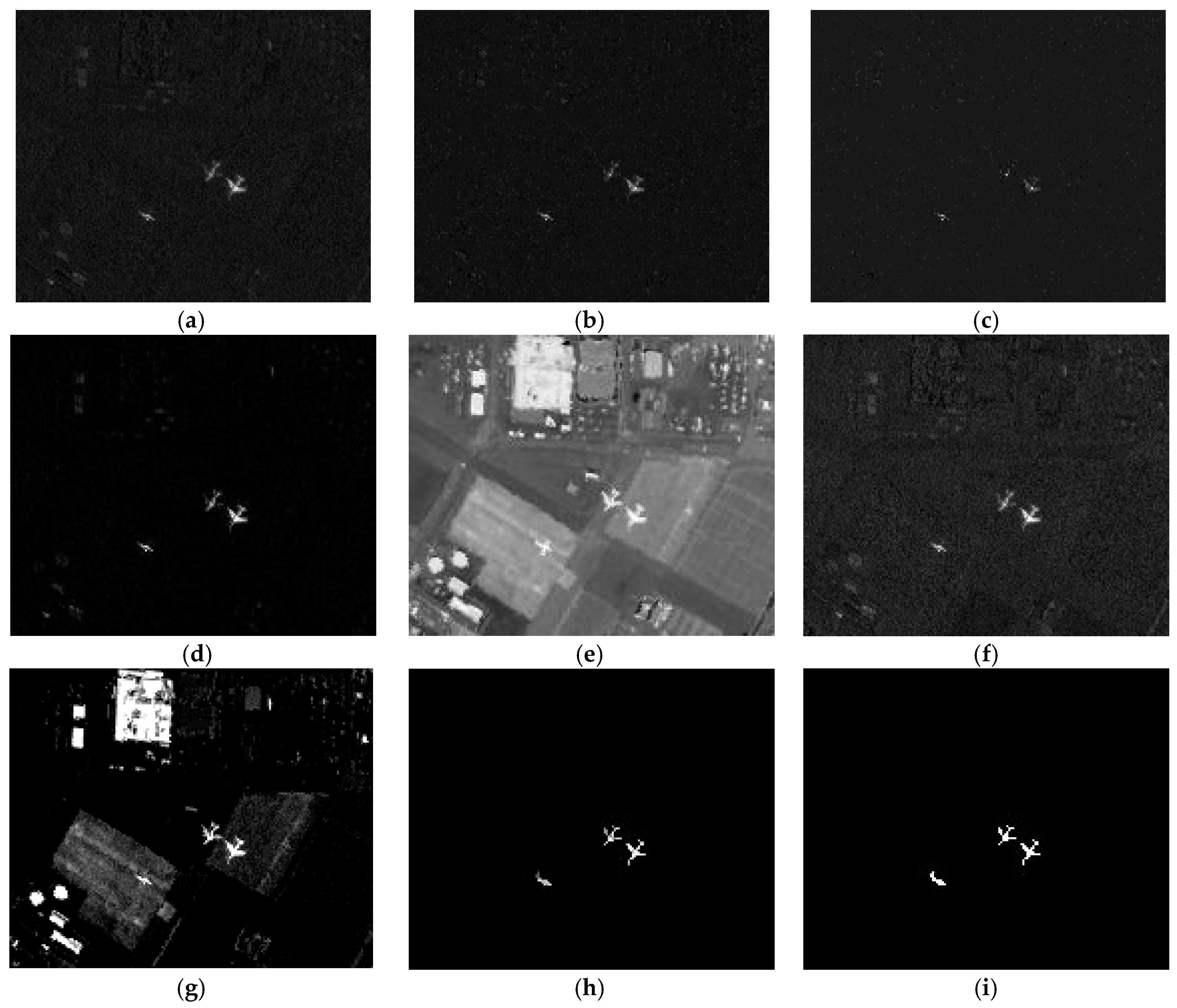
In Figure 9, we also compared the exist methods as the above tests. The detection results of hCEM still employed the first to third iterated layer. Comparing with CEM, SAM, and hCEM that have open source code, we tried the best to implement CE and MPCEM based on original CEM by ourselves. As for hyperspectral image data, all the methods performed better than they conducted detect on multispectral data. This might be due to the abundant spectral information of hyperspectral image data. In Figure 9, almost all these methods detected targets satisfied, except the SAM. The proposed method detected the target more effectively, by which the detected target was clearer and more complete for further analyzing. The hCEM can also remove most background, but the target was blurred at the same time. CEM and CE can present more significant target, while still reserving slight background. The MPCEM can extract the most clear and complete target, but the background was also significantly enhanced. The proposed method obtained the most clean background with relative clear and complete target, which performed more effectively on both multispectral and hyperspectral image data.
3.4. Experiment on the Fourth Dataset
Then, to further evaluate the proposed method, we test the SWCEM algorithm on another hyperspectral image data, which also come from AVIRIS. The spectral channels and available bands are all the same as Section 3.3. The spatial resolution is also 3.5 m for each band. From these hyperspectral data, we selected the scene with 53 × 122 pixels. Figure 10 presents the pseudo color image and reference data of the hyperspectral data. Since the targets in this scene are not so obvious, the selected part is relative small.
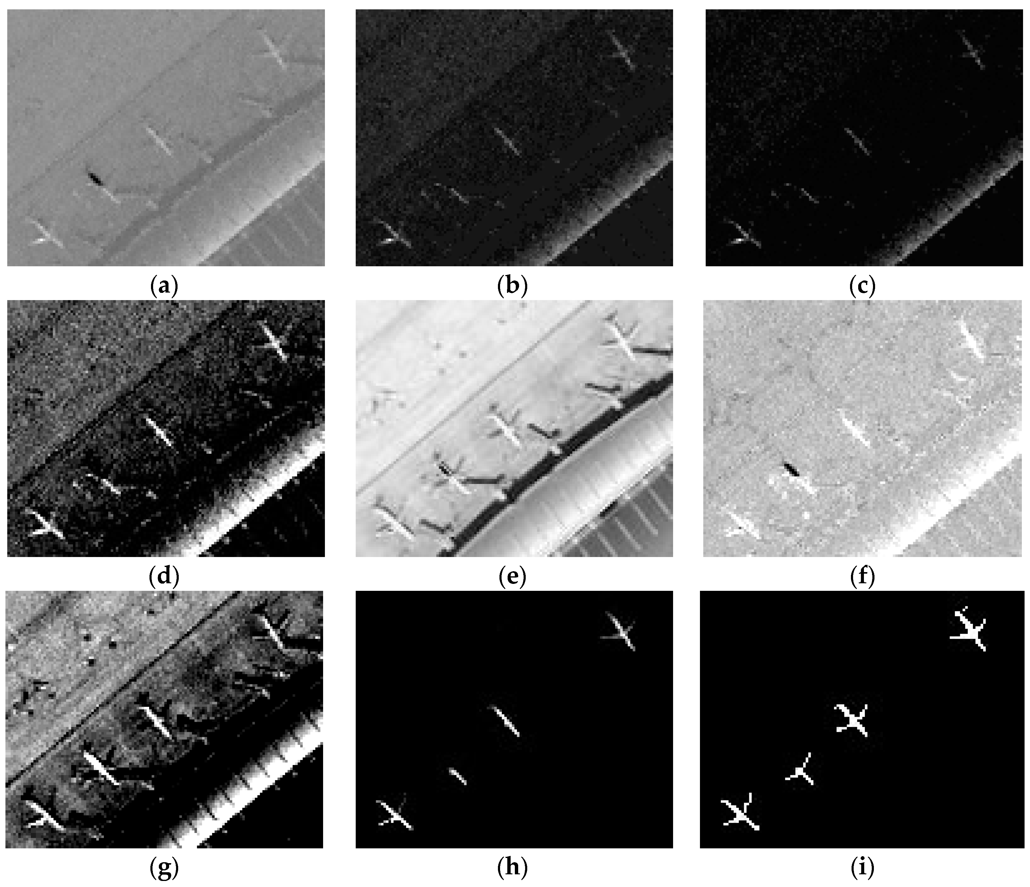
The detection results about the scene are presented in Figure 11. The first row is also the detection results of hCEM from first to third layer. As we can see, hCEM can hard detect target on this scene, as the resolution is not so satisfied. The same situations emerge in Figure 11d,f in the second row: the targets are almost lost by background noise. The SAM performed relatively better, because it is not sensitive to resolution and illumination, though it still reserved too many backgrounds. For MPCEM in Figure 11g, we find that it indeed presented good detection results. MPCEM can detect more clear targets than other methods on this scene. The proposed method performed impressively, as it can effectively suppress the background and detect more complete target. Although the hyperspectral image has higher spectral resolution, and the variability of spectral seems more complex, the proposed method can also effectively increase the difference between background and target spectrums. Furthermore, according to the fourth dataset, even if the image resolution is not satisfied, the proposed method is still robust and effective.
4. Discussion
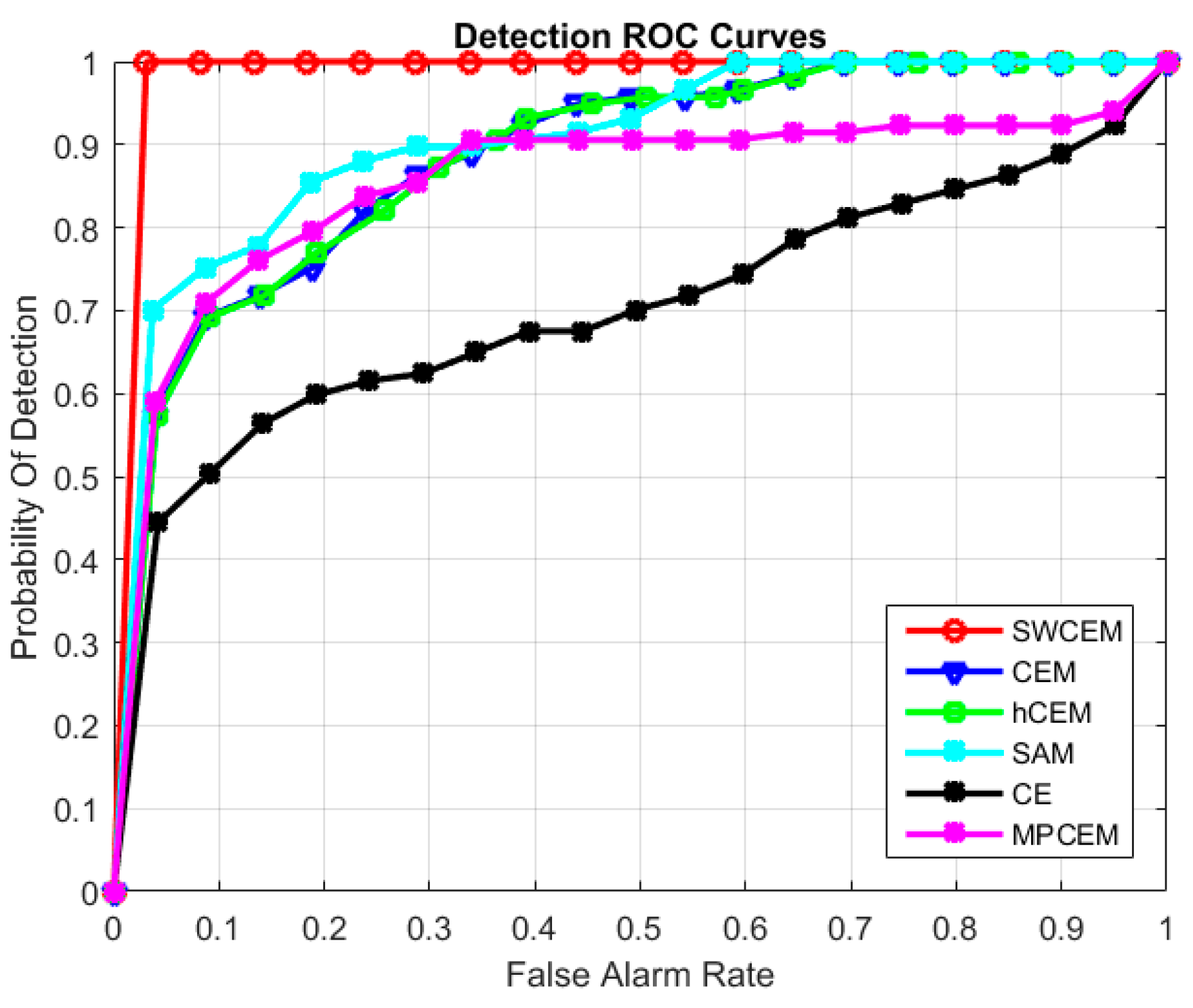
To further discuss the detection performance objectively, the receiver operating characteristic (ROC) [27,42] curves are employed to evaluate and analyze the experimental results. Several popular detection methods are also employed to validate the performance of the proposed method.
The ROC curves describe the varying relationship of detection probability and false alarm rate [27], i.e., describe the value of detection probability and false alarm rate corresponding to different threshold condition. The ROC curves provide a more intuitive and comprehensive performance evaluation method for target detection algorithms. The false alarm rate (Fa) and the probability of detection (Pd) are defined as follows:
where is the number of false alarm pixels, is the total number of background pixels, is the number of correct detection target pixels, and is the number of total true target pixels. The larger the area surrounded by the ROC curve is, the better the detection performance is.
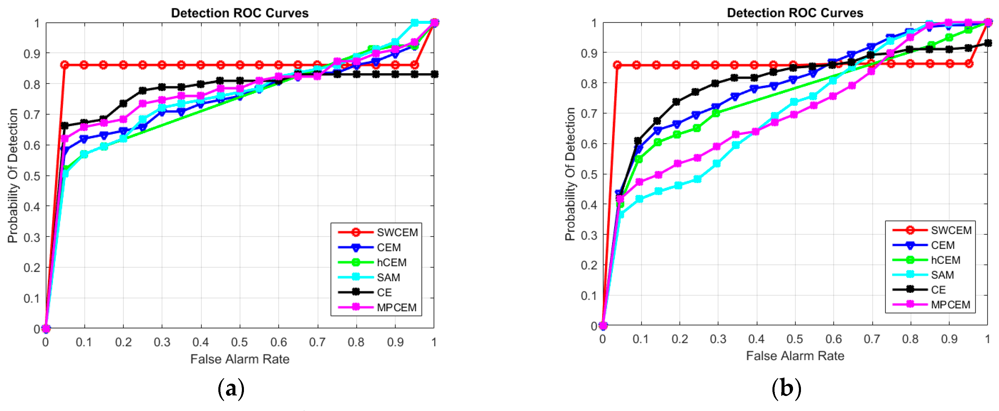
For more comprehensively, the evaluate procedure is still conducted on the above datasets, and the proposed method is compared with several classical and popular detection methods. Figure 12 shows the ROC curves of different algorithms on first dataset with two scenes. The ROC curves are built based on the same scene and hypothesis. The classical CEM, improved hCEM, popular SAM, and recently proposed CE, MPCEM are employed here to compare with the proposed methods. We can see that the proposed algorithm can obviously obtain higher detection probability at lower false alarm rates, and the ROC curves further prove that the SWCEM algorithm outperforms the other popular algorithms. For more intuitively, we calculated the area under ROC curves, which are shown in Table 1 and Table 2. We can conclude that the proposed method indeed achieves the highest area value, which means more significant performance.
Then, the ROC curves of different algorithms tested on the second dataset are presented in Figure 13. From the curves, we can obviously see that the proposed algorithm also can obtain better detection result than the other methods, with a flatter with more stable detection probability rate. We calculated the area under the ROC curves similarly, and recorded them in Table 3. In Table 3, the proposed method also covers the largest area, which effectively improves the detection performance of the classical CEM and outperforms the other methods.
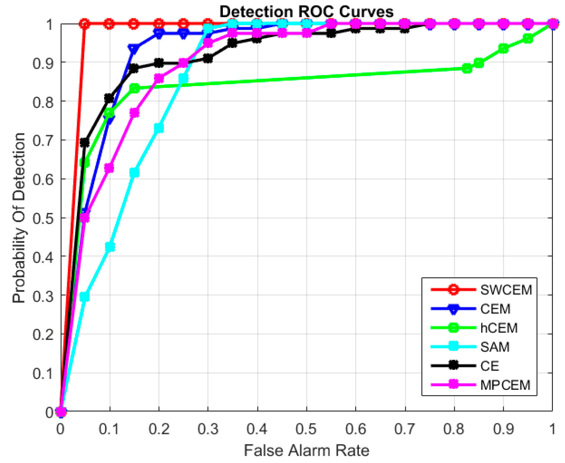
We then present the ROC curves of all the methods on the third and fourth dataset in Figure 14 and Figure 15. All the curves are nearer the upper left corner in Figure 14, as the third dataset possesses relatively more obvious target characteristics. Furthermore, we find that the proposed SWCEM algorithm can still achieved the best detection result coherently with the first two datasets, and the ROC curve of the proposed method presents more competitive detection rate under the same false alarm rate. Under the same condition, the areas under the ROC curves of these methods are shown in Table 4 and Table 5. These area values can further verify the effectiveness of the proposed method, which report highest value in the table.
According to the above discussion, we can find that these statistical results give the perspective that the proposed SWCEM is more effective and robust on detection task comparing with the exist works. It can achieve significant performance on different datasets under uniform hypothesis and parameters setting. The ROC curves and area value demonstrate the high detection sensitivity of the proposed method. Considering its complexity, we also analyzed the detection time of these methods, and the proposed SWCEM also reports competitive computation time compared to the existing methods, while only a little more than original CEM. This is because of the introduction of sparse weighted item, which needs to adaptively calculate and assign.
The method we proposed can be easily extended to multiple target detection tasks, with only a few constraints added. In our experiments, airplanes are very representative of the target, because the plane’s wing and back on the plane’s spectrum information is not very similar. It is like a multitasking detection task, and we have introduced two of different sparse constraints to accommodate this problem. These constraints can be manually labeled or acquired from labeled data, and the proposed method adaptively computes multiple weights by using sparse encoding constraints from different destinations. Once the constraint is changed, the target function should be rebuilt and recalculated to achieve different target detection results. How to balance these constraints is a problem to be considered in the future. In addition, the detection efficiency can be further improved by introducing some fast optimization methods.
5. Conclusions
This paper presents a new sparse weighted-based constrained energy minimization (SWCEM) algorithm for target detection in remote sensing images. The sparse representation is introduced to obtain the recovery residual of each pixel, which can describe the similarity between pixels and target. Then, the exponential weighting function is designed to generate adaptive weights for pixels based on recovery residual. Weighted pixels generate a new image data to the detector, which can effectively suppress the complex background while keeping the target significant, and the proposed detection procedure will more significantly detect the target from complex background. A series of experiments is conducted on different datasets with the proposed SWCEM algorithm, and the experimental results illustrate more competitive performance when compared with both classical and recent target detection methods.
Acknowledgments
This research was supported partially by the National Natural Science Foundation of China (Grant No. 61571343), the Fundamental Research Funds for the Central Universities (Grant No. JB140225), and the Specialized Research Fund for the Doctoral Program of Higher Education of China (Grant Nos. 20120203120009 and 20121401120015).
Author Contributions
Ying Wang and Jie Li conceived and designed the experiments; Zhaobin Cui performed the experiments; Miao Fan and Ying Wang analyzed the data; Ying Wang contributed reagents/materials/analysis tools; and Ying Wang and Miao Fan wrote the paper.
Conflicts of Interest
The authors declare no conflicts of interest.
References
- Han, J.; Zhang, D.; Cheng, G. Object detection in optical remote sensing images based on weakly supervised learning and high-level feature learning. IEEE Trans. Geosci. Remote Sens. 2015, 53, 3325–3337. [Google Scholar] [CrossRef]
- Wang, Q.; Meng, Z.; Li, X. Locality Adaptive Discriminant Analysis for Spectral-Spatial Classification of Hyperspectral Images. IEEE Geosci. Remote Sens. Lett. 2017, 14, 2077–2081. [Google Scholar] [CrossRef]
- Gao, J.; Wang, Q.; Yuan, Y. Embedding structured contour and location prior in siamesed fully convolutional networks for road detection. In Proceedings of the IEEE International Conference on Robotics and Automation, Singapore, 29 May–3 June 2017; pp. 1–12. [Google Scholar]
- Wang, Q.; Gao, J.; Yuan, Y. A Joint Convolutional Neural Networks and Context Transfer for Street Scenes Labeling. IEEE Trans. Intell. Trans. Syst. 2017. [CrossRef]
- Han, J.; Zhou, P.; Zhang, D. Efficient, simultaneous detection of multi-class geospatial targets based on visual saliency modeling and discriminative learning of sparse coding. ISPRS J. Photogramm. Remote Sens. 2014, 89, 37–48. [Google Scholar] [CrossRef]
- Li, X.; Zhang, S.; Pan, X. Straight road edge detection from high-resolution remote sensing images based on the ridgelet transform with the revised parallel-beam Radon transform. Int. J. Remote Sens. 2010, 31, 5041–5059. [Google Scholar] [CrossRef]
- Liu, W.; Yamazaki, F.; Vu, T.T. Automated vehicle extraction and speed determination from QuickBird satellite images. IEEE J. Sel. Top. Appl. Earth Obs. Remote Sens. 2011, 4, 75–82. [Google Scholar] [CrossRef]
- Karakaya, A.; Yüksel, S.E. Target detection in hyperspectral images. In Proceedings of the IEEE International Conference on Signal Processing and Communication Application, Zonguldak, Turkey, 16–19 May 2016; pp. 1501–1504. [Google Scholar]
- Manolakis, D.; Marden, D.; Shaw, G.A. Hyperspectral image processing for automatic target detection applications. Linc. Lab. J. 2003, 14, 79–116. [Google Scholar]
- Manolakis, D.; Siracusa, C.; Shaw, G. Hyperspectral subpixel target detection using the linear mixing model. IEEE Trans. Geosci. Remote Sens. 2001, 39, 1392–1409. [Google Scholar] [CrossRef]
- Kerekes, J.P.; Baum, J.E. Spectral imaging system analytical model for subpixel object detection. IEEE Trans. Geosci. Remote Sens. 2002, 40, 1088–1101. [Google Scholar] [CrossRef]
- Stefanou, M.S.; Kerekes, J.P. Image-derived prediction of spectral image utility for target detection applications. IEEE Trans. Geosci. Remote Sens. 2010, 48, 1827–1833. [Google Scholar] [CrossRef]
- Manolakis, D.; Shaw, G. Detection algorithms for hyperspectral imaging applications. IEEE Signal Process. Mag. 2002, 19, 29–43. [Google Scholar] [CrossRef]
- Manolakis, D.; Lockwood, R.; Cooley, T.; Jacobson, J. Is there a best hyperspectral detection algorithm? In Proceedings of the SPIE Defense, Security, and Sensing, Orlando, FL, USA, 13–17 March 2009. [Google Scholar]
- Robey, F.C.; Fuhrmann, D.R.; Kelly, E.J. A CFAR adaptive matched filter detector. IEEE Trans. Aerosp. Electron. Syst. 1992, 28, 208–216. [Google Scholar] [CrossRef]
- Chen, W.S.; Reed, I.S. A new CFAR detection test for radar. Digit. Signal Process. 1991, 1, 198–214. [Google Scholar] [CrossRef]
- Kruse, F.A.; Lefkoff, A.B.; Boardman, J.W. The spectral image processing system (SIPS)-interactive visualization and analysis of imaging spectrometer data. Remote Sens. Environ. 1993, 44, 145–163. [Google Scholar] [CrossRef]
- Fakiris, E.; Papatheodorou, G.; Geraga, M.; Ferentinos, G. An Automatic Target Detection Algorithm for Swath Sonar Backscatter Imagery, Using Image Texture and Independent Component Analysis. Remote Sens. 2016, 8, 373. [Google Scholar] [CrossRef]
- Wang, J.; Chang, C.I. Independent component analysis-based dimensionality reduction with applications in hyperspectral image analysis. IEEE Trans. Geosci. Remote Sens. 2006, 44, 1586–1600. [Google Scholar] [CrossRef]
- Farrand, W.H.; Harsanyi, J.C. Mapping the distribution of mine tailings in the Coeur d′Alene River Valley, Idaho, through the use of a constrained energy minimization technique. Remote Sens. Environ. 1997, 59, 64–76. [Google Scholar] [CrossRef]
- Harsanyi, J.C. Detection and Classification of Subpixel Spectral Signatures in Hyperspectral Image Sequences. Ph.D. Thesis, University of Maryland Baltimore County, Baltimore, MD, USA, 1993. [Google Scholar]
- Bidon, S.; Besson, O.; Tourneret, J.Y. The adaptive coherence estimator is the generalized likelihood ratio test for a class of heterogeneous environments. IEEE Signal Process. Lett. 2008, 15, 281–284. [Google Scholar] [CrossRef] [Green Version]
- Yang, S.; Shi, Z.; Tang, W. Robust hyperspectral image target detection using an inequality constraint. IEEE Trans. Geosci. Remote Sens. 2015, 53, 3389–3404. [Google Scholar] [CrossRef]
- Geng, X.; Yang, W.; Ji, L.; Wang, F.; Zhao, Y. The match filter (MF) is always superior to constrained energy minimization (CEM). Remote Sens. Lett. 2017, 8, 696–702. [Google Scholar] [CrossRef]
- Yang, S.; Shi, Z. SparseCEM and SparseACE for hyperspectral image target detection. IEEE Geosci. Remote Sens. Lett. 2014, 11, 2135–2139. [Google Scholar] [CrossRef]
- Zou, Z.; Shi, Z. Hierarchical suppression method for hyperspectral target detection. IEEE Trans. Geosci. Remote Sens. 2016, 54, 330–342. [Google Scholar] [CrossRef]
- Geng, X.; Ji, L.; Sun, K. Clever eye algorithm for target detection of remote sensing imagery. Isprs J. Photogramm. Remote Sens. 2016, 114, 32–39. [Google Scholar] [CrossRef]
- Wang, Y.; Huang, S.; Liu, D.; Wang, H. A Target Detection Method for Hyperspectral Imagery Based on Two-Time Detection. J. Indian Soc. Remote Sens. 2017, 45, 239–246. [Google Scholar] [CrossRef]
- Ren, H.; Du, Q.; Chang, C.I. Comparing between constrained energy minimization based approaches for hyperspectral imagery. In Proceedings of the IEEE Workshop on Advances in Techniques for Analysis of Remotely Sensed Data, Greenbelt, MD, USA, 27–28 October 2003; pp. 244–248. [Google Scholar]
- Du, Q.; Ren, H.; Chang, C.I. A study between orthogonal subspace projection and generalized likelihood ratio test in hyperspectral image analysis. In Proceedings of the IEEE International Geoscience and Remote Sensing Symposium, Toronto, ON, Canada, 24–28 June 2002. [Google Scholar]
- Harsanyi, J.C.; Chang, C.I. Hyperspectral image classification and dimensionality reduction: An orthogonal subspace projection approach. IEEE Trans. Geosci. Remote Sens. 1994, 32, 779–785. [Google Scholar] [CrossRef]
- Scharf, L.L.; Friedlander, B. Matched subspace detectors. IEEE Trans. Signal Process. 1994, 42, 2146–2157. [Google Scholar] [CrossRef]
- Sun, W.; Jiang, M.; Li, W.; Liu, Y. A Symmetric Sparse Representation Based Band Selection Method for Hyperspectral Imagery Classification. Remote Sens. 2016, 8, 238. [Google Scholar] [CrossRef]
- Zhang, Y.; Du, B.; Zhang, L. A sparse representation-based binary hypothesis model for target detection in hyperspectral images. IEEE Trans. Geosci. Remote Sens. 2015, 53, 1346–1354. [Google Scholar] [CrossRef]
- Chen, Y.; Nasrabadi, N.M.; Tran, T.D. Hyperspectral image classification using dictionary-based sparse representation. IEEE Trans. Geosci. Remote Sens. 2011, 49, 3973–3985. [Google Scholar] [CrossRef]
- Chen, Y.; Nasrabadi, N.M.; Tran, T.D. Hyperspectral image classification via kernel sparse representation. IEEE Trans. Geosci. Remote Sens. 2013, 51, 217–231. [Google Scholar] [CrossRef]
- Chen, Y.; Nasrabadi, N.M.; Tran, T.D. Simultaneous joint sparsity model for target detection in hyperspectral imagery. IEEE Geosci. Remote Sens. Lett. 2011, 8, 676–680. [Google Scholar] [CrossRef]
- Chang, C.I. Multiparameter receiver operating characteristic analysis for signal detection and classification. IEEE Sens. J. 2010, 10, 423–442. [Google Scholar] [CrossRef]
- Chen, Y.; Nasrabadi, N.M.; Tran, T.D. Sparse representation for target detection in hyperspectral imagery. IEEE J. Sel. Top. Signal Process. 2011, 5, 629–640. [Google Scholar] [CrossRef]
- Niu, Y.; Wang, B. Hyperspectral target detection using learned dictionary. IEEE Geosci. Remote Sens. Lett. 2015, 12, 1531–1535. [Google Scholar]
- Tropp, J.A.; Gilbert, A.C. Signal recovery from random measurements via orthogonal matching pursuit. IEEE Trans. Inf. Theory 2007, 53, 4655–4666. [Google Scholar] [CrossRef]
- Nocedat, J.; Wright, S.J. Numerical Optimization; Springer: New York, NY, USA, 2000. [Google Scholar]
- Peng, X.; Lu, C.; Yi, Z.; Tang, H. Connections between Nuclear-Norm and Frobenius-Norm-Based Representations. IEEE Trans. Neural Netw. Learn. Syst. 2016, PP, 1–7. [Google Scholar] [CrossRef] [PubMed]
- Peng, X.; Lu, J.; Yi, Z.; Yan, R. Automatic Subspace Learning via Principal Coefficients Embedding. IEEE Trans. Cybern. 2017, 47, 3583–3596. [Google Scholar] [CrossRef] [PubMed]
- Peng, X.; Yu, Z.; Yi, Z.; Tang, H. Constructing the L2-Graph for Robust Subspace Learning and Subspace Clustering. IEEE Trans. Cybern. 2017, 47, 1053–1066. [Google Scholar] [CrossRef] [PubMed]
Figure 1.
Shape of exponential function with different parameter λ.

Figure 2.
The first scene of the Xianyang Airport: (a) three band false color composite; and (b) reference data.
Figure 2.
The first scene of the Xianyang Airport: (a) three band false color composite; and (b) reference data.

Figure 3.
The second scene of the Xianyang Airport: (a) three band false color composite; and (b) reference data.
Figure 3.
The second scene of the Xianyang Airport: (a) three band false color composite; and (b) reference data.

Figure 4.
Detection results of the first scene of Xianyang Airport: (a–c) results of the hierarchical Constrained energy minimization (hCEM) algorithm for the first to third layers; (d) results of Constrained energy minimization (CEM) algorithm; (e) results of Spectral angle mapper (SAM) algorithm; (f) results of Clever eye (CE) algorithm; (g) results of MPCEM (Matrix principal Constrained energy minimization) algorithm; (h) results of Sparse weighted-based Constrained energy minimization (SWCEM) algorithm; and (i) reference data.

Figure 5.
Detection results of the second scene of Xianyang Airport: (a–c) results of the hCEM algorithm for the first to third layers; (d) results of CEM algorithm; (e) results of SAM algorithm; (f) results of CE algorithm; (g) results of MPCEM algorithm; (h) results of SWCEM algorithm; and (i) reference data.

Figure 6.
The image of the Chanba Area: (a) three band false color composite; and (b) reference data.
Figure 6.
The image of the Chanba Area: (a) three band false color composite; and (b) reference data.

Figure 7.
Detection results of the Chanba Area: (a–c) results of the hCEM algorithm for the first to third layers; (d) results of CEM algorithm; (e) results of SAM algorithm; (f) results of CE algorithm; (g) results of MPCEM algorithm; (h) results of SWCEM algorithm; and (i) reference data.
Figure 7.
Detection results of the Chanba Area: (a–c) results of the hCEM algorithm for the first to third layers; (d) results of CEM algorithm; (e) results of SAM algorithm; (f) results of CE algorithm; (g) results of MPCEM algorithm; (h) results of SWCEM algorithm; and (i) reference data.

Figure 8.
The image of AVIRIS: (a) pseudo color display of AVIRIS Dataset 1; and (b) reference data.
Figure 8.
The image of AVIRIS: (a) pseudo color display of AVIRIS Dataset 1; and (b) reference data.

Figure 9.
Detection results of the AVIRIS data: (a–c) results of the hCEM algorithm for the first to third layers; (d) results of CEM algorithm; (e) results of SAM algorithm; (f) results of CE algorithm; (g) results of MPCEM algorithm; (h) results of SWCEM algorithm; and (i) reference data.
Figure 9.
Detection results of the AVIRIS data: (a–c) results of the hCEM algorithm for the first to third layers; (d) results of CEM algorithm; (e) results of SAM algorithm; (f) results of CE algorithm; (g) results of MPCEM algorithm; (h) results of SWCEM algorithm; and (i) reference data.

Figure 10.
The image of AVIRIS: (a) pseudo color display of AVIRIS Dataset 2; and (b) reference data.
Figure 10.
The image of AVIRIS: (a) pseudo color display of AVIRIS Dataset 2; and (b) reference data.

Figure 11.
Detection results of the AVIRIS data: (a–c) results of the hCEM algorithm for the first to third layers; (d) results of CEM algorithm; (e) results of SAM algorithm; (f) results of CE algorithm; (g) results of MPCEM algorithm; (h) results of SWCEM algorithm; and (i) reference data.
Figure 11.
Detection results of the AVIRIS data: (a–c) results of the hCEM algorithm for the first to third layers; (d) results of CEM algorithm; (e) results of SAM algorithm; (f) results of CE algorithm; (g) results of MPCEM algorithm; (h) results of SWCEM algorithm; and (i) reference data.

Figure 12.
Receiver operating characteristic (ROC) curves on the two scenes: (a) ROC curves of different algorithms on the first scene; and (b) ROC curves of different algorithms on the second scene.
Figure 12.
Receiver operating characteristic (ROC) curves on the two scenes: (a) ROC curves of different algorithms on the first scene; and (b) ROC curves of different algorithms on the second scene.

Figure 13.
ROC curves of different algorithms on the Chanba Area data.

Figure 14.
ROC curves of different methods on AVIRIS Dataset 1.

Figure 15.
ROC curves of different methods on AVIRIS Dataset 2.


Table 1.
The area surrounded by ROC curves of different algorithms on the first scene.
| CEM | hCEM | SAM | CE | MPCEM | SWCEM | |
|---|---|---|---|---|---|---|
| AUC | 0.7937 | 0.7534 | 0.7063 | 0.8174 | 0.7741 | 0.8492 |
Table 2.
The area surrounded by ROC curves of different algorithms on the second scene.
| CEM | hCEM | SAM | CE | MPCEM | SWCEM | |
|---|---|---|---|---|---|---|
| AUC | 0.7937 | 0.7534 | 0.7063 | 0.7957 | 0.7105 | 0.8474 |
Table 3.
The area surrounded by ROC curves of different algorithms on the Chanba Area data.
| CEM | hCEM | SAM | CE | MPCEM | SWCEM | |
|---|---|---|---|---|---|---|
| AUC | 0.9306 | 0.8361 | 0.8709 | 0.9197 | 0.9005 | 0.9756 |
Table 4.
The area surrounded by ROC curves of different algorithms on the AVIRIS Dataset 1.
| CEM | hCEM | SAM | CE | MPCEM | SWCEM | |
|---|---|---|---|---|---|---|
| AUC | 0.9578 | 0.9571 | 0.9637 | 0.9578 | 0.9619 | 0.9765 |
Table 5.
The area surrounded by ROC curves of different algorithms on the AVIRIS Dataset 2.
| CEM | hCEM | SAM | CE | MPCEM | SWCEM | |
|---|---|---|---|---|---|---|
| AUC | 0.8847 | 0.8832 | 0.9069 | 0.7020 | 0.8541 | 0.9845 |
© 2017 by the authors. Licensee MDPI, Basel, Switzerland. This article is an open access article distributed under the terms and conditions of the Creative Commons Attribution (CC BY) license (http://creativecommons.org/licenses/by/4.0/).
Share and Cite
MDPI and ACS Style
Wang, Y.; Fan, M.; Li, J.; Cui, Z. Sparse Weighted Constrained Energy Minimization for Accurate Remote Sensing Image Target Detection. Remote Sens. 2017, 9, 1190. https://0-doi-org.brum.beds.ac.uk/10.3390/rs9111190
AMA Style
Wang Y, Fan M, Li J, Cui Z. Sparse Weighted Constrained Energy Minimization for Accurate Remote Sensing Image Target Detection. Remote Sensing. 2017; 9(11):1190. https://0-doi-org.brum.beds.ac.uk/10.3390/rs9111190
Chicago/Turabian StyleWang, Ying, Miao Fan, Jie Li, and Zhaobin Cui. 2017. "Sparse Weighted Constrained Energy Minimization for Accurate Remote Sensing Image Target Detection" Remote Sensing 9, no. 11: 1190. https://0-doi-org.brum.beds.ac.uk/10.3390/rs9111190
Note that from the first issue of 2016, this journal uses article numbers instead of page numbers. See further details here.