A New Fully Gap-Free Time Series of Land Surface Temperature from MODIS LST Data


1
Mundialis GmbH & Co. KG, 53111 Bonn, Germany
2
Department of Earth Observation Sciences, ITC-Faculty of Geo-Information Science and Earth Observation, University of Twente, 7522 Enschede, The Netherlands
*
Author to whom correspondence should be addressed.
Remote Sens. 2017, 9(12), 1333; https://0-doi-org.brum.beds.ac.uk/10.3390/rs9121333
Submission received: 30 September 2017
/
Revised: 13 December 2017
/
Accepted: 14 December 2017
/
Published: 20 December 2017
(This article belongs to the Section Remote Sensing Image Processing)
Abstract
:Temperature time series with high spatial and temporal resolutions are important for several applications. The new MODIS Land Surface Temperature (LST) collection 6 provides numerous improvements compared to collection 5. However, being remotely sensed data in the thermal range, LST shows gaps in cloud-covered areas. We present a novel method to fully reconstruct MODIS daily LST products for central Europe at 1 km resolution and globally, at 3 arc-min. We combined temporal and spatial interpolation, using emissivity and elevation as covariates for the spatial interpolation. The reconstructed MODIS LST for central Europe was calibrated to air temperature data through linear models that yielded R2 values around 0.8 and RMSE of 0.5 K. This new method proves to scale well for both local and global reconstruction. We show examples for the identification of extreme events to demonstrate the ability of these new LST products to capture and represent spatial and temporal details. A time series of global monthly average, minimum and maximum LST data and long-term averages is freely available for download.
1. Introduction
Remote sensing based time series are becoming increasingly available, and this tendency will continue to grow not only because of new Earth observation satellites being launched, but because of the availability of new methods to harmonize their data [1,2] and reconstruct incomplete records [3,4,5,6,7] along with the growing demand of different sectors for the monitoring of environment, analysis of trends and patterns, and forecasting. In this scenario, air temperature is as an essential climatic and ecological driver, one of the most important variables in climate research and global change. It controls many biological and physical processes between the hydrosphere, atmosphere and biosphere [8]. Therefore, the availability of spatially and temporally continuous temperature time series at high spatial and temporal resolution is crucial for a wide range of disciplines including hydrology, meteorology and ecology [9,10], as well as for numerous applications fields.
While meteorological stations can provide accurate air temperature measurements (near-surface temperature, usually measured about 2 m above ground), they only represent single locations with their immediate surrounding area of influence. Moreover, the distribution of meteorological stations is far from optimal for most areas of the world. This type of point data needs to be spatialized (usually performed through geostatistical approaches or thermodynamical modelling) to characterize regions. Regardless of the spatialization method used, unrepresentative smooth spatial patterns may occur due to the lack of dense data [11,12,13]. In the end, the obtained precision depends on the quality, representativeness and spatial distribution of the input network(s) of stations [12,13,14]. Besides, processing such data can be quite time-consuming regarding computation time (especially to obtain higher spatial resolution datasets), difficult to automate (i.e., data requires a lot of “curation”), and therefore, it is not easily updated with new incoming data [14,15,16].
Land surface temperature (LST) as recorded by remote sensing instruments on board of satellites, on the other hand, is intrinsically spatial and provides the spatial coverage that meteorological stations lack. As such, satellite LST is able to capture at greater detail local differences in temperature originating from varying meteorological conditions, environmental differences and/or active heat sources (e.g., urban areas, land cover classes) [15]. The most commonly used LST products are those from the MODerate resolution Imaging Spectroradiometer (MODIS) instruments on board of Terra and Aqua NASA satellites. The combination of these satellite data provides spatial estimates of LST at high temporal (four Earth coverages per 24 h; approximately 01:30, 10:30, 13:30, and 22:30, local solar time) and high spatial resolution (nominally 1 km) across the world [17,18]. Remotely sensed LST, however, as all remotely sensed data in the optical/thermal portions of the spectrum, suffers from cloud contamination, i.e., occurrence of gaps produced by cloud cover and/or presence of outliers in undetected cloudy pixels [5,19] which reduces the usage rate and hinders any subsequent interpretation [20]. The percentage of valid LST values varies in space and time depending on the region, but in any case, the gaps must be filled to render the data useful for other applications or research fields (e.g., for deriving climatic indices, modeling, etc.).
Previous LST related studies have attempted to obtain spatially and temporally continuous estimates of temperature for areas of varying sizes using different methods, time series of different lengths and different LST products. There have been two approaches aiming at two different outputs: (1) to use MODIS LST as one of the explanatory variables in statistical models to obtain gridded time series of air temperature [9,15,16,21,22]; and (2) to directly reconstruct LST products either with or without covariates [2,5,19,23,24]. In the first case, approaches go from linear regression models to more complex spatio-temporal regression-kriging interpolations, from regional (country scale) to global predictions and from only one to 10 years of output air temperature time series. In all of the first cases, these approaches use MODIS LST products (either daily or eight-day composites, both from Terra and Aqua satellites or only from Terra) to enhance the spatial detail attained with meteorological stations with the help of one or more predicting variables in a statistical model. In the second case, the reconstruction of satellite LST data, diverse approaches have been used. For example, a MODIS LST time series has been reconstructed and compressed using temporal Fourier transform by Scharlemann et al. [23] who processed MODIS LST at a full global extent for the years 2001 to 2005 and extracted parameters for the annual, bi-annual and tri-annual cycle through Fourier transform at a resolution of 1 km. Another temporal interpolation method replaced/estimated missing Aqua LST values with Terra LST values [24], however the resulting dataset still contained gaps. On the other hand, Neteler [19] used 3D spline interpolation to fully reconstruct LST (2000–2008, daily, at 200 m spatial resolution) for a small alpine region in northern Italy with an algorithm optimized for very complex topography. For this latter reason, the method could not be extended to larger areas, and motivated the study by Metz et al. [5], combining temporal averaging with multiple regression and spline interpolation to produce a seamless and gap-free daily reconstructed LST for Europe at 250 m spatial resolution for the period 2000–2013 (“EuroLST” dataset). For a summary of previous approaches to reconstruct LST time series, see Table 1 in Metz et al. [5].
All papers cited above have made use of LST MODIS collection 5. In 2017, NASA completed the reprocessing of the entire MODIS archive and made available a new collection 6 of MODIS products. This new version includes different kinds of fixes and improvements, including removal of cloud-contaminated LST from MODIS level 2 and 3 products; updated coefficients for the split-window algorithm; adjustments in the classification-based surface emissivity values, etc. [18]. On the software side, new methods became available in the last years for the gap-filling of time series. For example, the long standing free and open source software GRASS GIS [25,26], offers new enhanced modules and methods to efficiently handle and process huge amounts of geospatial time series data [27,28,29,30,31].
In this study, we present a new method to reconstruct MODIS LST collection 6 data that combines temporal interpolation to fill small gaps in time and spatial interpolation with covariates to fill the remaining gaps in space. We used a digital elevation model and one of the emissivity bands delivered along with MODIS LST products as covariates in the spatial interpolation step. The use of emissivity allows us to characterize the thermal properties of different land covers at the same temporal resolution at which we have LST records while providing complementary information to that contributed by elevation data, a well known predictor of temperature. To our knowledge, emissivity has not been used before in the reconstruction or interpolation of temperature surfaces. We applied the new method to the MOD11A1/MYD11A1 LST products for Central Europe (2003–2016) with a spatial resolution of 1 km, as well as to global LST products at 3 arc-min (nominally 5.6 km at the equator). Therefore, this new approach delivers seamless and gap-free LST time series at two different spatial resolutions with comparable satisfying quality and can easily be applied as-is to other parts of the world. Furthermore, it can be automated and continuously updated (with new incoming MODIS LST data) without much delay.
Having a long time series of daily observations allows for different aggregations and extraction of other (synthetic) variables. In this paper, we use the identification of extreme events to demonstrate how this new LST product covering a relatively short time span of 14 years is able to detect well-known anomalous events with high spatial and temporal detail.
2. Materials and Methods
2.1. Data
We used the MODIS LST products MOD11A1/MYD11A1 collection 6 acquired from the LP DAAC data pool (https://lpdaac.usgs.gov/dataset_discovery/modis/modis_products_table) starting with the year 2003, the first year fully covered by both products. These two products combined provide four LST values per day at a spatial resolution of nominally 1 km. We used the tiles h18v03, h18v04, h19v03, h19v04 covering central Europe (data provided in MODIS sinusoidal projection, the extents are 2223.9 km × 2223.9 km with a raster resolution of 926.6 m). The spatial coverage comprised a total of 5,760,000 pixels, of which 4,342,823 pixels were on land (75.4%). Additionally, we applied the same reconstruction method to the global MODIS LST products MOD11C1/MYD11C1 at a spatial resolution of 3 arc-min (approximately 5.6 km at the equator). As elevation model we used the Global Multi-resolution Terrain Elevation Data 2010 grids (GMTED2010; resolution 30 arc-s) available from the U.S. Geological Survey (https://lta.cr.usgs.gov/GMTED2010). Monthly ground meteo-station records of air temperature were obtained from the German Weather Service (DWD) for the year 2016 (the number of active DWD stations per month varied between 483 and 489, see Table 1 in the Results, Section 3.5). Land cover information was obtained from the MODIS product MCD12Q1 collection 051 for the year 2013 (which is the latest year and collection available at the time of writing), using land cover type 4: MODIS-derived Net Primary Production (NPP) scheme (spatial resolution: 500 m).
2.2. LST Reconstruction Method
All pixels with an LST error >3 K were filtered out using the corresponding MODIS LST QA layers (quality assurance layers in the MODIS LST HDF files). Thus missing values were all pixels for which no LST value had been produced as well as all pixels with an LST error >3 K. We used this rather liberal threshold because preliminary tests showed that a lower threshold for LST error would discard also LST values that appear to be correct. Therefore we decided to keep potentially valid LST values at the expense of including more outliers. Outlier filtering is performed at a later stage.
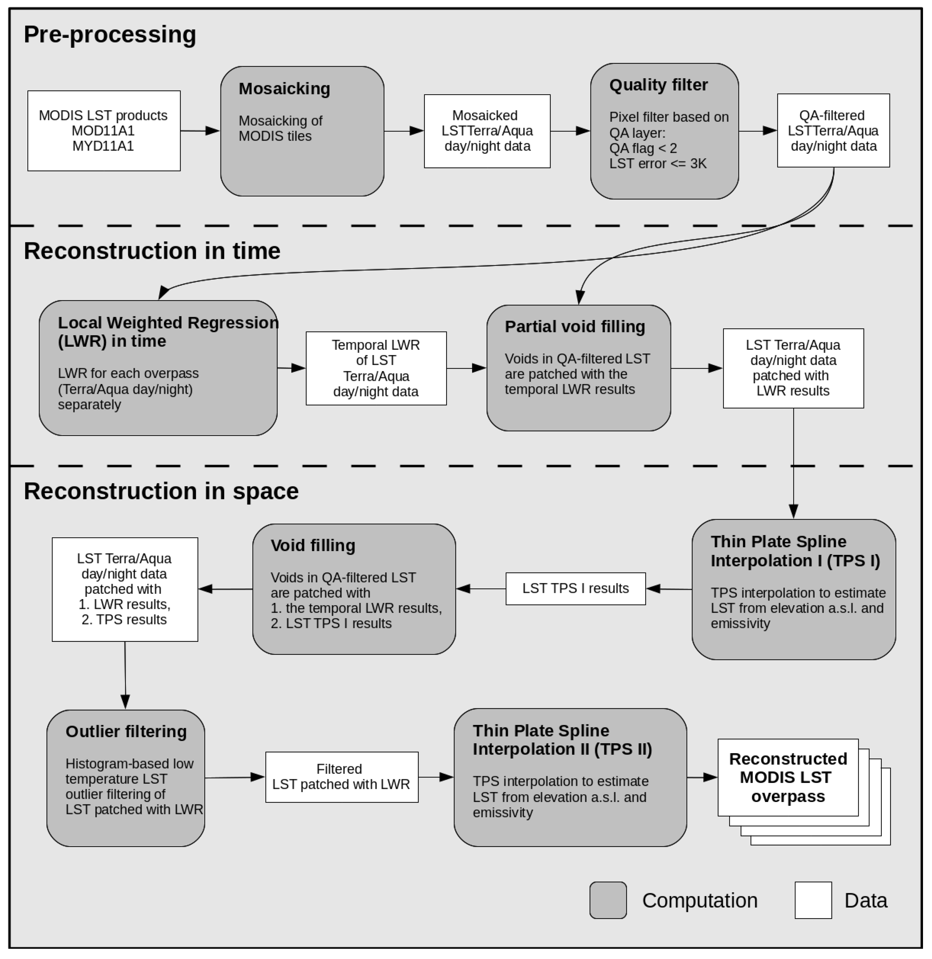
Variation of daily surface temperature can be quite high. Any interpolation in time should therefore allow for fast fluctuations and should avoid smoothing of the time series in order to preserve extreme events. For temporal interpolation we used local weighted regression (LWR; GRASS GIS add-on r.series.lwr [29,30]) with polynomial order 2, considering the five nearest neighbors in time. Since the intra-day and inter-day fluctuations might be mixed up in the interpolation by the existence of any missing values, we treated each daily time step (01:30, 10:30, 13:30 and 22:30) as a separate time series. Intra-day fluctuations in LST can vary considerably among days, i.e., day-time and night-time temperatures can be nearly identical or quite different. Therefore, temporal interpolation of all four daily overpasses together over several days would require a priori assumptions on intra-day fluctuations for each day separately, which are impossible to determine if none or only one observation for a certain day is available. There exist models based on diurnal temperature cycle, but those require several temperature measures per day (see, for example, Liu et al. [32]), which are not available in the case of MODIS sensors. Gaps larger than seven days were not interpolated and left as missing values. We used thin plate spline interpolation (TPS; GRASS GIS add-on r.resamp.tps [29,30]) with elevation data from GMTED2010 and band 31 emissivity from the MODIS LST products as covariates to fill any remaining gaps in space. For details on TPS, see [33,34,35]. Here we used an adaptive window size determined by the spatial distribution of the nearest 150 points. Preliminary tests showed that considering emissivity increased the contrast between urban areas, vegetated areas, and water bodies. Emissivity also exhibited missing values due to cloud cover. However, since emissivity does not change as long as land cover remains constant, it can be easily reconstructed with temporal interpolation. We used LWR with polynomial order 1, using the nearest 7 neighbors in time and filling gaps up to 30 days long to obtain gap-free emissivity that was then used as covariate in the spatial interpolation of LST. Low outliers were defined as values larger than Q3 + 1.5 × (Q3 – Q1), with Q1 and Q3 being the first and third quartile of reference data [5,19]. As reference data we used the time steps of the same day, the last time step of the previous day and the first time step of the next day. The workflow of our MODIS LST reconstruction method is illustrated in Figure 1. Importantly, since valid pixels in the MODIS Land Surface Temperature products represent clear-sky conditions, our reconstruction method as well as most other studies attempting to fill missing values in LST, also represent clear-sky conditions.
To evaluate the robustness of the reconstruction method, we created gaps of different sizes in the raw LST data, reconstructed these gaps and compared the resulting reconstructed LST values to the raw LST values. These differences of the simulated gaps were then compared to the differences of the originally reconstructed LST values to the raw LST values.
2.3. Software
For mosaicking, we used the GDAL tool gdalbuildvrt (GDAL, http://www.gdal.org). All further processing was performed in GRASS GIS 7.2 [25,26]. The MODIS LST time series was processed on a Linux cluster computing system, managed by the “Son of Grid Engine” job scheduler (SGE, https://arc.liv.ac.uk/trac/SGE).
2.4. Assessment of LST Derived Indicators: Identification of Extreme Events
Considering climatological standards, our time series is quite short, spanning only 14 years so far. Therefore, we wanted to test if it is possible to identify extreme events with this short time series as reference.
Extreme events in climate science are usually defined by three criteria, i.e., rarity, intensity and severity. Definitions of “rare” vary, but an extreme weather event would normally be as rare or more rare than the 10th or the 90th percentile. Rarity can thus be assessed with the calculation of the corresponding quantile for the current observation according to a reference time series. A quantile of 0.5 means that the current observation is equal to the median, values larger than 0.5 mean larger than median and values smaller than 0.5 smaller than median. A value of 0.9 for example means that the current observation is equal to the 90% percentile of the reference time series. Intensity, in the context of extreme events, refers to their magnitude, i.e., events that have large magnitude deviations from the norm. Intensity can be assessed with standardized anomalies: the difference of the current observation to the long-term average, divided by the long-term standard deviation. These standardized anomalies are thus the number of standard deviations away from the average, with the sign indicating if the current observation is larger or smaller than the average. Finally, severity is related to the socio-economic losses that a rare and intense event may cause [36].
3. Results
The newly developed LST reconstruction method was applied to central Europe covered by four MOD11A1/MYD11A1 tiles with approximately 1 km resolution and furthermore globally applied to MOD11C1/MYD11C1 images with a resolution of 3 arc-min. Regarding central Europe, there are 20,456 time steps covering the years 2003 to 2016 (four records per day), corresponding to 384 GiB of selected raw data (i.e., LST, quality assurance, and emissivity layers).
The results consist of two parts: (1) an analysis of the MODIS LST products used here and of the LST reconstruction method; and (2) the identification of extreme events as an exemplary use case.
3.1. Missing Values
For the four tiles covering central Europe during 2003–2016, 61.4% of the temperature values were missing from the original MODIS LST collection 6 products (after filtering with the corresponding QA flags as described in the Methods Section 2.2). The smallest percentages of missing values occurred at high altitudes and along edges of water bodies. The water bodies themselves had a slightly higher percentage of missing values than their edges, probably due to fog over water bodies. The highest percentage of missing values appeared in low-lying inland areas away from oceans such as central Germany.
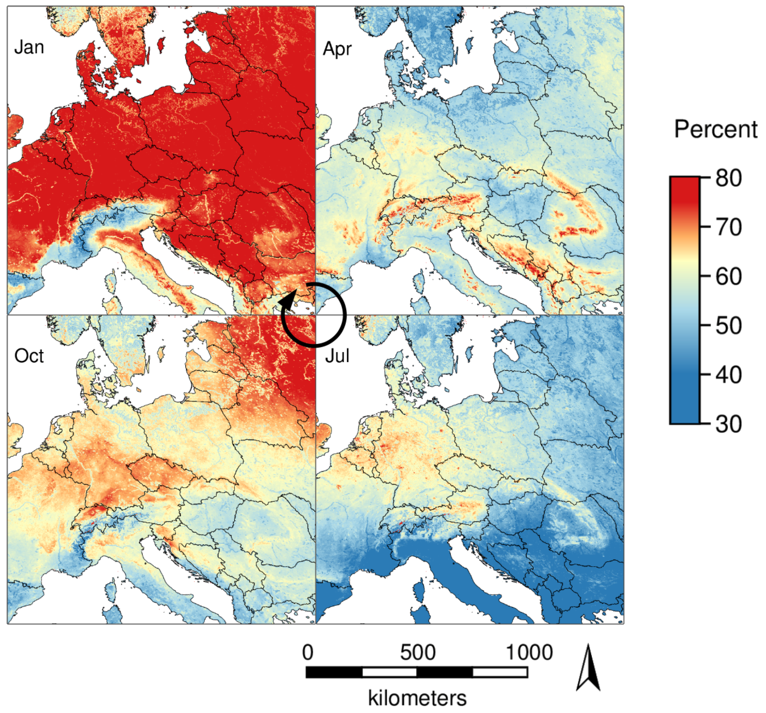
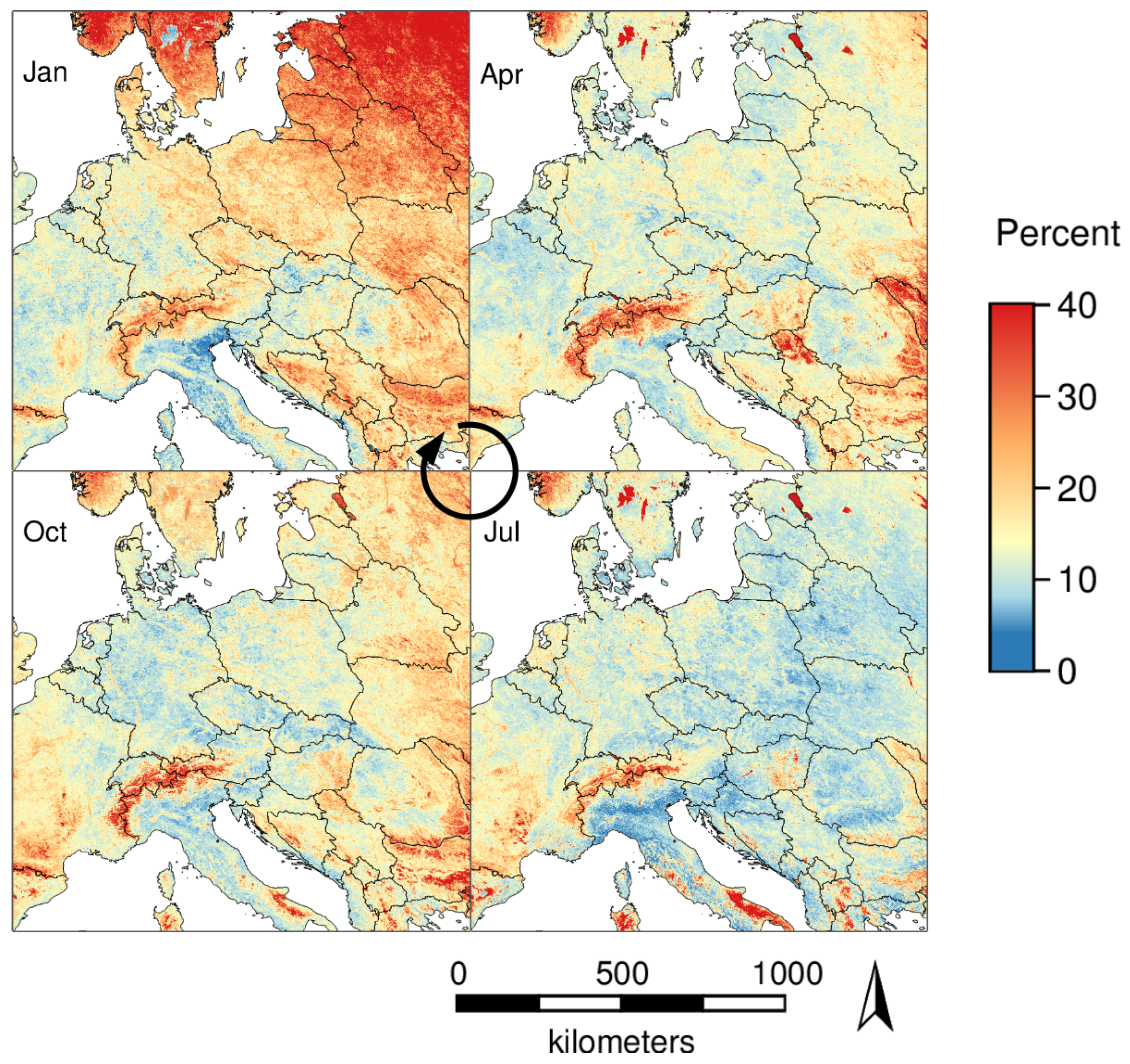
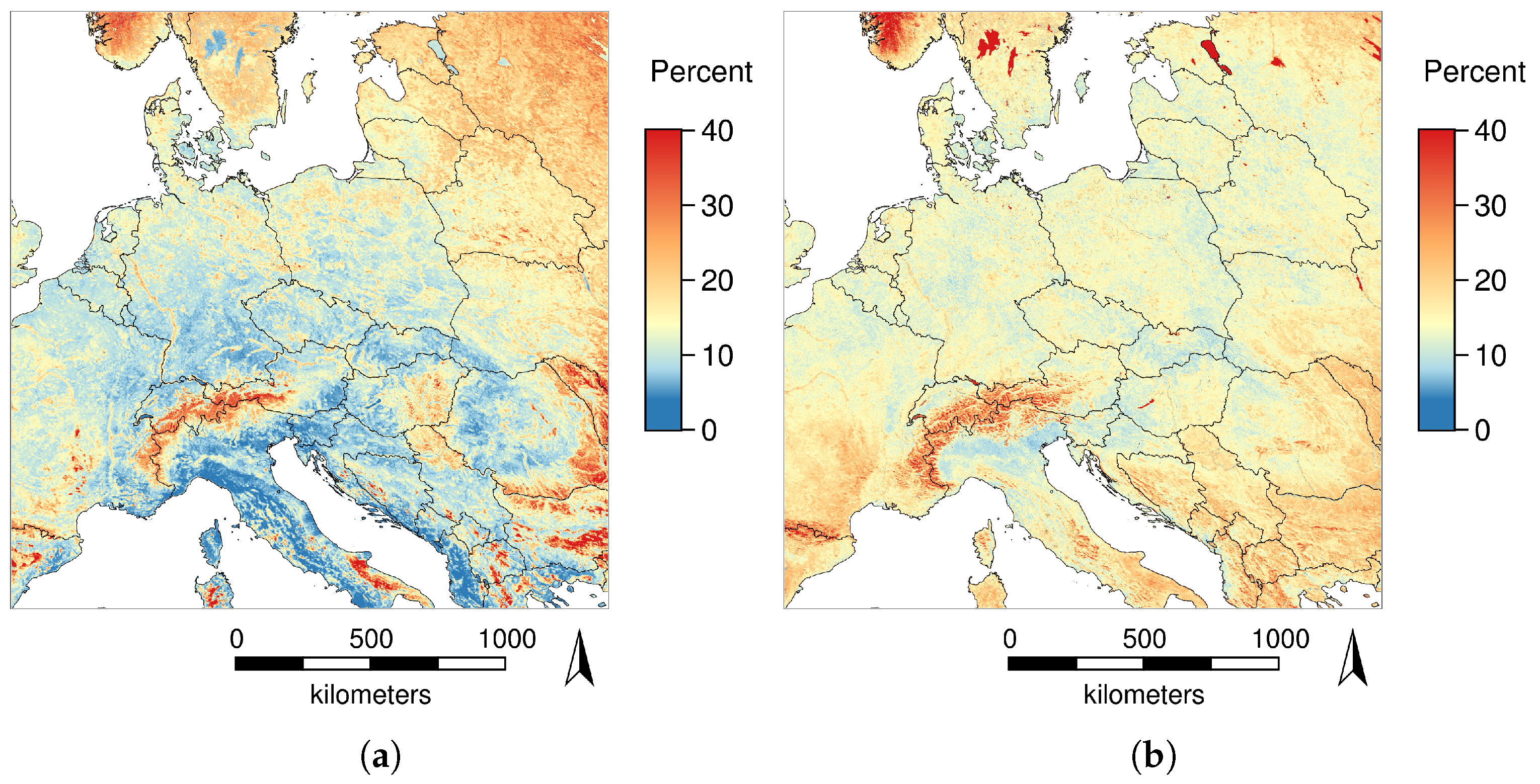
An inspection of months aggregated over all available years showed that most missing values appeared in the winter months November–February (71–74%), and least missing values appeared in the summer months June–September (49–55%). A comparison of missing values in the months January, April, July, and October (average over all years) revealed that not only the percentage of missing values but also their spatial distribution differs between months (Figure 2). In January (74.4% missing), most missing values appeared in lowland areas (up to 1000 m a.s.l.). In April (56.9% missing), most missing values were observed at higher altitudes. In July (49.8% missing), the lowest percentage of missing values appeared in southern Europe and, in October (62.3% missing), a high percentage of missing values appeared in north-eastern Europe and parts of France, Switzerland, Germany, and Austria. The seasonal differences in the amount of missing LST values is most probably caused by climate conditions of the current region (central Europe). For other parts of the world, different seasonal patterns in the amount of missing LST values are to be expected. To understand if missing values were equally common and equally distributed in different times of the day, the number of missing values was counted for each pixel and each time of the day over all processed days (Figure 3 with 01:30 and 13:30). High altitude areas such as the Alps showed few (<40%) missing values at night and average (50–60%) missing values during the day, while northern parts of central Europe had about 10% more missing values during the day than at night.
Temporal interpolation with LWR reconstructed 68% of all missing values. In summer, more missing values could be temporally reconstructed than in winter, e.g., averaged over all years, 85% of missing values were reconstructed in August and 48% in January.
An example for the temporal and spatial reconstruction of missing values is given in Figure 4. The proportion of pixels filled with temporal interpolation varies between time steps, depending on the coverage of nearby days.
3.2. Outliers
For the four tiles covering central Europe from 2003 to 2016, 5.9% of all surface temperature values were identified as outliers in the original MODIS LST products. Generally, the highest percentage of outliers appeared at high altitudes and in water bodies. Regarding monthly outlier counts aggregated over years, most outliers were detected in the months April–July (6.2–6.4%), and the lowest percentage of outliers was detected in the months November–February (5.2–5.6%).
Figure 5 shows a comparison of the percentage of outliers in the months January (5.2% outliers), April (6.4% outliers), July (6.4% outliers), and October (6.0% outliers) aggregated over the years 2003 to 2016. In January, most outliers appeared in northern and north-eastern Europe. A notable exception are water bodies where only few outliers were detected. In April and July, the highest percentage of outliers appeared at high altitudes and over water bodies. In October, outliers appeared at high altitudes and also in eastern and northern Europe, while water bodies did not show peculiar percentages of outliers.
To compare the four different overpass times per day in terms of outlier occurrence, the outlier counts were aggregated over all days and years for each overpass time of the day, and then divided by the corresponding number of valid LST pixels. The most obvious difference in the percentage of outliers was observed over water bodies where only few outliers at night and many outliers during the day occurred, e.g., in southern Sweden and at the border between Estonia and Russia (Figure 6).
3.3. Effect of Emissivity
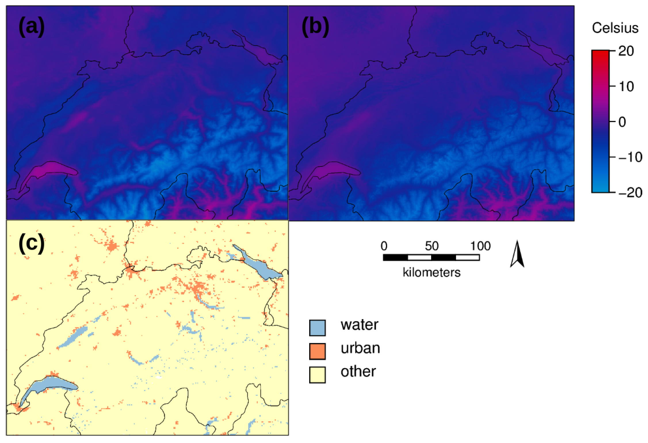
Since emissivity differs among land cover types, particularly among urban areas, water bodies, and vegetated areas, we compared reconstructed LST data with land cover types from the MODIS product MCD12Q1. The effects of emissivity on LST reconstruction are clearly visible for urban areas and larger water bodies. In winter, both urban areas and water bodies appear hotter during the day due to the high specific heat capacity when compared to both vegetated areas and the result of LST reconstruction without using the emissivity layer (Figure 7).
3.4. Simulation of Missing Data
We evaluated the robustness of the reconstruction method by creating holes of different sizes in the raw LST data and then reconstructing these holes. The difference of the reconstruction over simulated gaps to the raw data was then compared to the difference of the original reconstruction (only outlier filtering, no gap filling) to the raw data (Table 1). As test data, we used an area without gaps in the Aqua daytime overpass at 13:30 for 23 June 2016. While the difference of the original reconstructed LST values to the raw data was always less than 0.5 K, the results over simulated gaps where between 1.2 and 2.7 K smaller than the raw LST values.
3.5. Calibration to Station Data
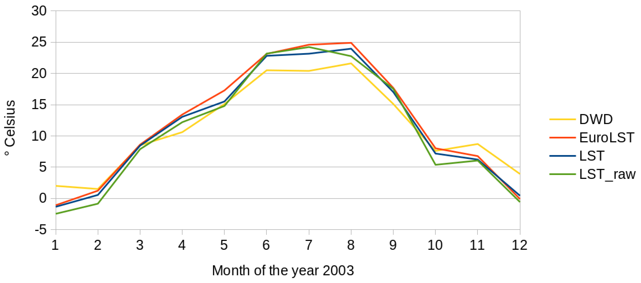
We compared time series of the new LST reconstruction considering emissivity (this paper), the corresponding raw data of the MODIS 11A1 products, the old “EuroLST” reconstruction not considering emissivity [5], and air temperature records from the German Weather Service (DWD) ground stations, using monthly averages for the year 2003 for the city of Bonn, Germany. Both reconstruction methods are closely following the raw LST data, but tend to be higher than the raw LST data due to the removal of low outliers. It appears that values of the new LST reconstruction are equal to or slightly lower than those of the old LST reconstruction. All LST time series are slightly above the values of ground station records in summer and slightly lower than ground station records in winter (Figure 8), indicating that for each time step, surface temperature needs to be individually calibrated to air temperature because the bias of surface temperature to air temperature is different for each time step.
We used monthly averages for 2016 as test data for calibrating reconstructed LST to air temperature recorded at ground stations. Air temperature values were obtained from DWD meteorological station records, which varied for 2016 from 483 to 489 stations among different months. Because the bias of surface to air temperature is different for each time step, surface temperature was calibrated to air temperature for each month separately with a linear model (Table 2). The influence of elevation as additional variable in the linear models was also investigated. We used R2, root mean square error (RMSE), and Akaike information criterion (AIC) to evaluate the goodness of the calibration. Calibration succeeded with R2 in the range of 0.83 to 0.91 and RMSE in the range of 0.38 to 0.64, excluding December. The month of December presented by far the lowest R2 (0.71), the highest RMSE (0.90), and the highest AIC (−91.3). The percentages of missing values and outliers were not unusually high for December 2016. The poor match between MODIS LST and the reconstruction method and air temperature recorded at ground stations for this month could be caused by a failure of the reconstruction method or by errors in the ground station data. Generally, elevation improved the calibration slightly. For a few months (April, September, October, and December), the improvements when including elevation were considerable (ΔR2 > 0.2).
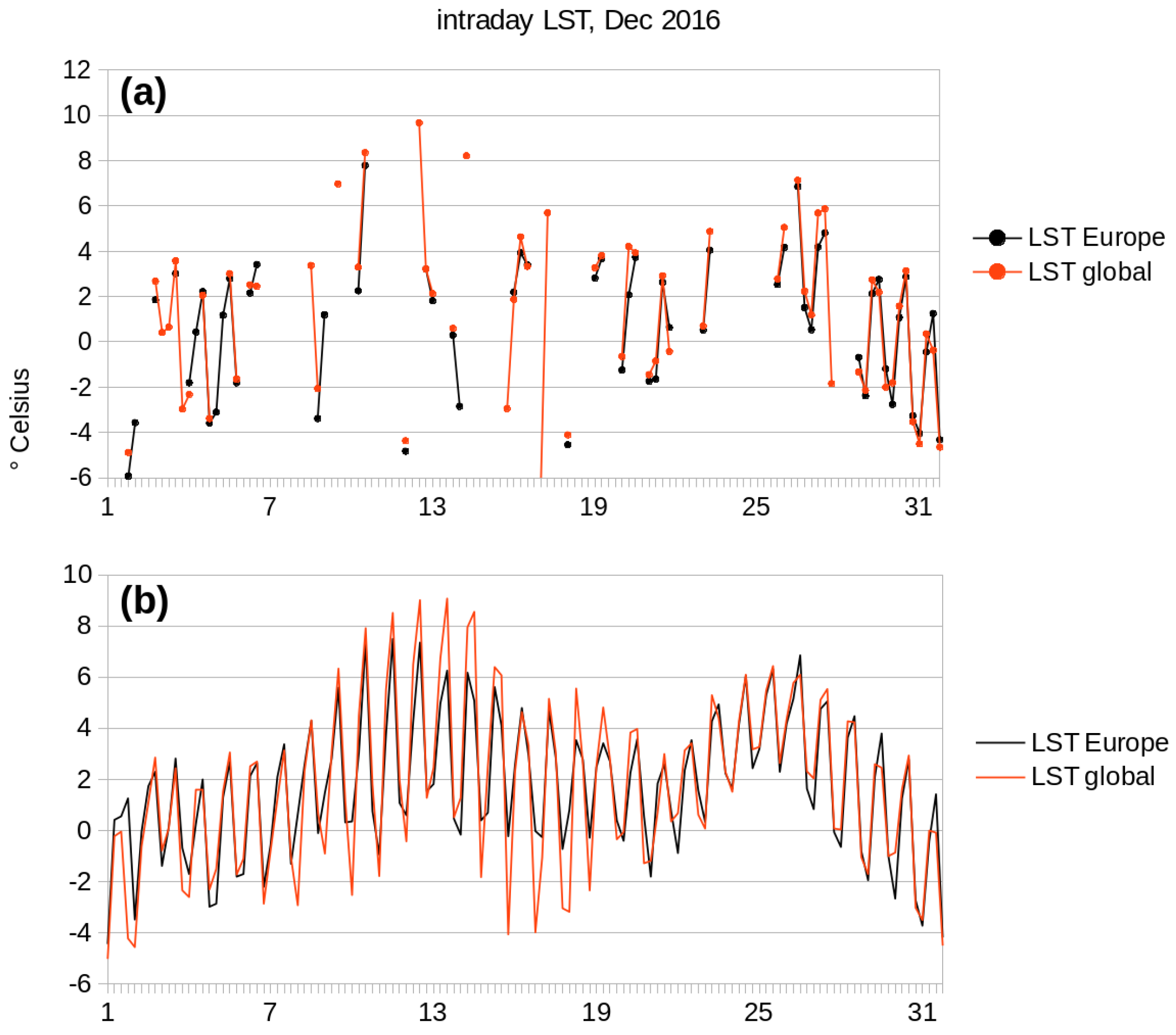
The new LST reconstruction method was applied to both central Europe using the MODIS products MOD11A1/MYD11A1 and globally using the MODIS products MOD11C1/MYD11C1. These MODIS LST products are created independent of each other. Comparing an intra-day time series for December 2016 revealed some overshoots in the global reconstruction (Figure 9b), where the global reconstruction had lower values at night and higher values during the day. These differences could well be caused by differences in the raw data (Figure 9a).
3.6. Extreme Events
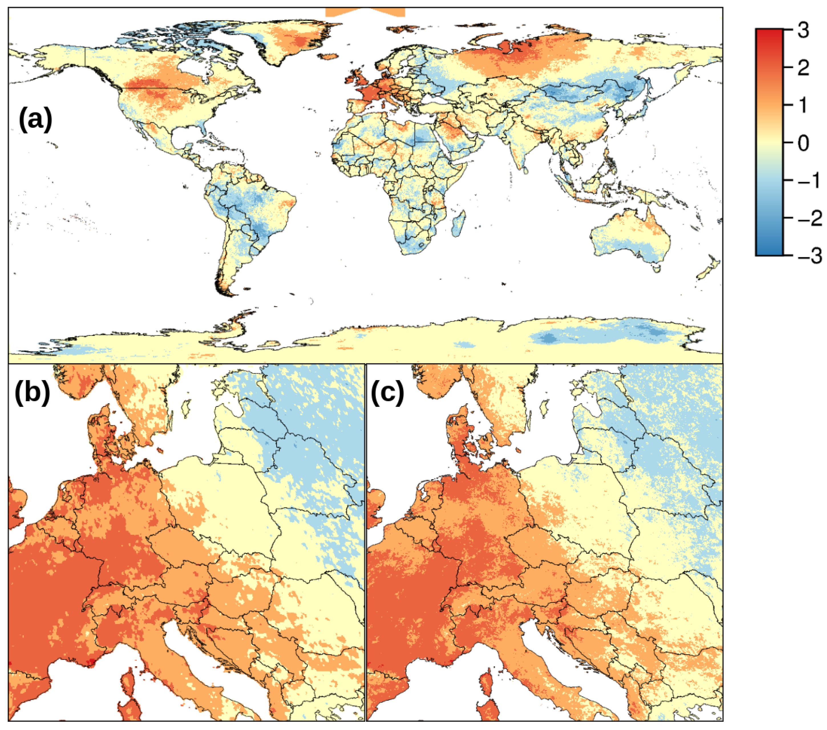
Extreme events can be identified by comparing current observations to an adequate reference time series. The reconstructed LST time series spanning 14 years is relatively short compared to climatological standards. Nevertheless, extreme events can be identified using this time series as reference. Extreme events can be highly localized in both space and time (a small area affected in a short period of time). The high spatial and temporal resolution of the reconstructed MODIS LST time series allows to detect such localized events as illustrated with the example of the heat wave in Europe in August 2003. This heat wave is visible in both the global and the European reconstructed LST time series (Figure 10). Both time series were able to show the high intensity of the heat wave with a very similar spatial pattern despite different spatial resolutions (nominally 5.6 km vs. nominally 1 km). Notably, the global time series (Figure 10a) shows that this heat wave was restricted to western Europe, illustrating that the reference time series spanning 14 years is long enough for spatial discrimination.
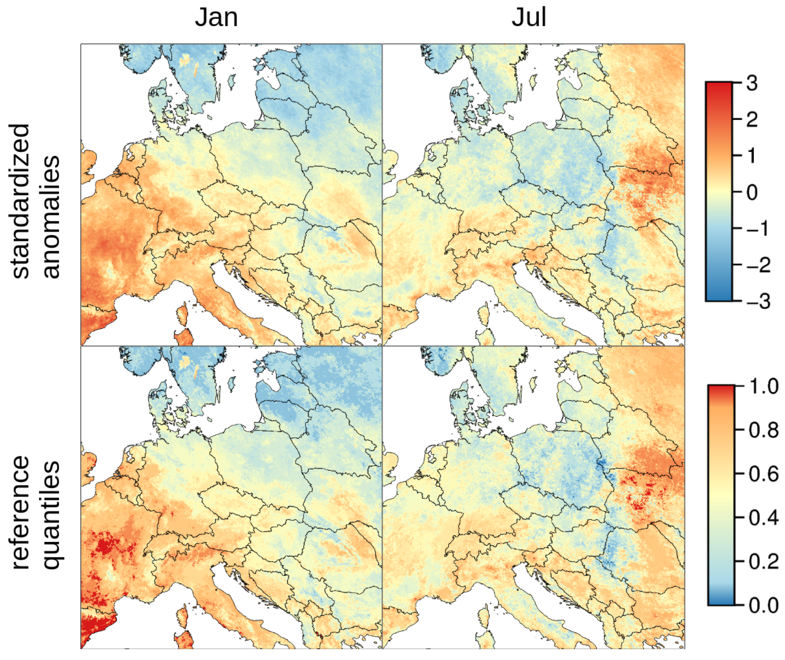
Next, we compared average monthly temperatures for January and July 2016 with the time series for the years 2003–2016 with regard to intensity and rarity. For January 2016, temperatures in western and southern parts of our study area were considerably higher than the 2003–2016 average and median (Figure 11). These high temperatures were thus an intense and rare event. In July 2016, eastern parts of our study area were warmer than the 2003–2016 average and median. Similar analyses on extreme events can also be performed on shorter time scales such as weeks or days.
4. Discussion
Land surface temperature (LST) is a key variable in the physical processes of surface energy and water balance at different scales [37,38]. As such, many research fields and applications, namely evapotranspiration, climate change, hydrology, vegetation monitoring, urban climate, public health, among others, require gap-free time series of this variable as inputs to better understand the spatio-temporal changes of different study targets [39,40,41,42].
In this paper, we presented a new method to obtain a fully gap-free time series of gridded daily surface temperature from MODIS collection 6 LST products (tiled MOD11A1/MYD11A1 data at 1 km resolution and global MOD11C1/MYD11C1 data at 3 arc-min resolution). The spatial support has been enhanced by using elevation and emissivity as covariates. This resulted in plausible differences among distinct land cover types (e.g., cities and water bodies) and also between low and high lying areas. The former were evident when we compared reconstructed LST including and omitting emissivity as covariate in the spatial interpolation step (Figure 1). By using one of the emissivity bands delivered with the MODIS LST products, we were able to account for spatial differences and temporal changes in land cover, thus catching for example seasonal changes due to snow cover or loss of leaves in trees. This would not have been the case if we would have used constant LULC maps produced annually (i.e., MCD12Q1 of which the production ended with the year 2013).
The highest percentage of missing values in central Europe was observed in the month of January (average based on 2003–2016). While this is probably an expected result given the climatic conditions common of that month in central Europe, it means that short-term fluctuations in temperature are probably not well represented for gaps that are large both in time and in space, eliminating any possible unrecorded short-term fluctuations. Interpolation of gaps that are small in time or space can preserve short-term fluctuations. A 68% of all missing values present in MODIS LST products were interpolated in time through LWR, while the remaining gaps were filled by means of TPS in the spatial interpolation step. The fact that there were more missing values during day than at night might be explained by the MODIS cloud detection algorithm that uses thermal and reflective bands for day overpasses, but only thermal bands for cloud detection at night, i.e., clouds are more easily detected during the day than at night [43,44]. The difference in the percentages of missing values among water bodies and their borders might also be related to the MODIS cloud detection algorithm that uses different spectral thresholds for different types of covers [45]. Therefore, if the land cover layer used is not up-to-date or water bodies change their size, differences in cloud detection over water bodies and their borders might be expected. This was observed by Kotarba [43] while analyzing MODIS collection 5 cloud product for the period 2004–2009 over Poland. However, they detected more clouds over water bodies than over water body borders. According to the authors, the approach used by the MODIS project for operational production of level 3 cloud data (used afterwards for other level 3 products such as LST) tends to over-estimate cloud amount by 6.5% in Europe (annually). In MODIS collection 6 some of the artifacts (decreased and spatially biased data availability) have apparently been reduced but not eliminated [46].
A high percentage of outliers was observed over water bodies in April and July when outlier percentages were aggregated per month, and at 13:30 when outlier percentages were aggregated per overpass time. Considering that water bodies do not change their temperature quickly (i.e., within a day), it is possible that the applied outlier detection might have resulted in false positives for water bodies, particularly at mid-day (13:30) and in summer, when land surfaces are typically hotter than water bodies. On the other hand, water bodies are frequently covered by clouds or fog, but not that many missing values were detected over water bodies as compared to other surfaces. Therefore, the observed higher percentage of outliers over water bodies might be explained by undetected clouds (a task marked as difficult in MOD35 ATBD). These undetected clouds will have significantly lower surface temperature and thus are identified as outliers by our method. This might partially explain why the percentage of outliers detected was higher over water bodies, but it does not fully explain why outliers were more common in summer months in which water bodies should not be so frequently covered by clouds or fog [45]. However, if those cells were indeed covered by clouds but not detected [47], it is expected that they are filtered as outliers given the much lower temperature of clouds. Outlier detection remains a challenge and will be the focus of future improvements.
In the standard MOD/MYD11 LST and emissivity products, emissivities are assigned a priori based on land cover classification maps, i.e., the MCD12Q1 products. The latter product however was only generated until 2013. Therefore, some differences can be expected in places where LULC have changed to a drastically different cover in terms of emissivity. In the estimation of emissivity for MOD/MYD11 products, some other adjustments are made for the thermal infrared bidirectional reflectance distribution function (TIR BRDF), snow (from MOD10_L2 product), and green vs. senescent vegetation. This a priori approach is known to perform well for surfaces where emissivity can be correctly assigned based on the classification, i.e., it is best suited for land-cover types such as dense evergreen canopies, lake surfaces, snow, and most soils, all of which have stable emissivities error levels known to be within 0.01. However, it is significantly less reliable over arid and semi-arid regions [48]. Furthermore, errors in LST estimation may be introduced when the emissivity changes from day to night observation (e.g., due to condensation or dew), sudden natural changes (e.g., due to precipitation, wildfires), and from undetected nighttime cloud.
A LST time series reconstructed from remotely sensed records such as MODIS LST products, including the one we are presenting here, provides more spatial detail than gridded air temperature time series interpolated from ground station data (point observations), not only for central Europe with a relatively dense coverage, but more importantly also for other areas of the world with a lower density of ground stations. Commonly used climatic datasets with a comparable spatial resolution are WorldClim (http://worldclim.org/, [49]), and CHELSA (http://chelsa-climate.org/, [50]). These datasets, however, provide long-term statistics for past time periods such as the average for the years 1970–2000 for average monthly temperatures and not up-to-date time series with, e.g., monthly average temperature for the year 2016, not to mention daily temperature time series. Therefore, while highly used, most of the times they do not match the time frame of the phenomenon under study (see for example [51]). The long-term summaries we provide might be used to estimate the same temperature-based bioclimatic variables as those provided by WorldClim or CHELSA datasets.
We have demonstrated that our reconstructed LST time series is capable of identifying extreme events such as the well known heat wave that affected central Europe in 2003. LST might also be used to detect/monitor (surface) Urban Heat Islands (UHI) [52] either by estimating the difference in LST between urban areas and their rural surroundings (see Tomlinson et al. [53] and references therein) or by estimating the number of consecutive tropical nights from night-time LST [40]. Further use cases might include for example, the field of agriculture. Here, growing degree day (GDD) maps are relevant for the phenological assessment of budburst, flowering and crop maturing. GDD maps derived from reconstructed MODIS LST maps can account for local variations, i.e., they are likely to provide more detail. In addition, seasonal gradient maps (intra-annual short term trends) are of interest for agriculture. Furthermore, using MODIS LST time series, the shift of the upper forest limits may be assessed, likewise the suitability for the presence of tree (or other plants) species in terms of sensitivity to temperature. In the vast areas of permafrost, on the other hand, where almost no meteorological stations are available, MODIS LST data may be used to determine the duration of phases over 0 °C and their spatial extent [54]. Moreover, for applications that require higher spatial detail, the method that we present allows enhancing the spatial resolution and detail of the reconstructed LST with the use of a higher resolution elevation model as covariate in the TPS interpolation. However, this enhancement of the spatial resolution will affect only areas with diverse topography [5,19].
The new LST reconstruction method presented here improves over our previous LST reconstruction [5] in various ways. It requires less external data: previously climatic data and elevation, now only elevation. The temporal interpolation has been improved to better represent short-term fluctuations: previously weighted average, now local weighted regression (LWR) with order 2. We preferred LWR [55] over HANTS [56] or Fourier transforms (as used in [23] and others) because HANTS and Fourier transforms are only suitable to detect seasonal and long-term fluctuations with a regular pattern. LWR in turn is able to represent and preserve also irregular short-term fluctuations, particularly when used with polynomial order 2 or 3. Furthermore, the spatial interpolation has been improved by using TPS [33,34,35] instead of bspline interpolation with Tykhonov regularization [57]: TPS interpolation preserves existing values which can be optionally smoothed, whereas bspline always smoothes existing values. Moreover, the integration of covariates into TPS interpolation can further improve the results. Regarding spatial interpolation, the most important change is that no longer a fixed interpolation window is used, but instead an adaptive window, accounting for gaps of different size in the spatial domain. Using an adaptive window instead of a fixed window helps to reduce artifacts.
The entire workflow presented here was carried out with the open source geospatial suites GDAL and GRASS GIS along with newly published GRASS GIS add-on modules [29,30]. Therefore, the procedure can be replicated for other areas of interest and the reconstructed LST time series can be continuously updated with newly arriving data. The new LST reconstruction method scales well both locally (sub-continental) with a spatial resolution of nominally 1 km, and globally with a spatial resolution of 3 arc-min. Importantly, the reconstructed time series can be kept up-to-date with commodity hardware (processing one month takes about one day with an 7th generation Intel Core i5). The workflow could also be used to reconstruct other LST time series, for example the AVHRR LST time series from NOAA satellites or the Sentinel-3 SLSTR, which would extend the temporal coverage of the MODIS LST time series.
5. Conclusions
In this paper, we present a novel method to gap-fill LST time series at sub-continental and global scale. In total, more than 20,000 maps were reprocessed to obtain a gap-free daily time series of LST as well as aggregated products at 1 km and 3 arc-min resolution. We have shown the potential of our method and resulting LST time series spanning so far 14 years for the identification of extreme events. Moreover, such a long time series of daily observations is relevant for numerous applications in environmental monitoring, agriculture, urban planning and public health.
Finally, the use of free data and of open source suites guarantees the reproducibility of the proposed method along with the possibility to apply it to other areas and future LST time series. Global monthly reconstructed minimum, average, and maximum LST data (2003–2016) are available from https://www.mundialis.de/lst/ and Zenodo (http://0-doi-org.brum.beds.ac.uk/10.5281/zenodo.1115666) in GeoTIFF format.
Acknowledgments
The MODIS LST V006 data products were retrieved from the online Data Pool, courtesy of the NASA Land Processes Distributed Active Archive Center (LP DAAC), USGS/Earth Resources Observation and Science (EROS) Center, Sioux Falls, South Dakota, https://e4ftl01.cr.usgs.gov. Some map colors are based on http://www.ColorBrewer2.org, by Cynthia A. Brewer, Penn State. We thank the three anonymous reviewers for their suggestions on an earlier version of the manuscript.
DWD data were retrieved from the Deutscher Wetterdienst (DWD) Climate Data Center (CDC) at ftp://ftp-cdc.dwd.de/pub/CDC.
Author Contributions
M.M. and V.A. developed the methodology supported by M.N. and performed the analysis. M.M., V.A., and M.N. wrote the manuscript.
Conflicts of Interest
The authors declare no conflict of interest.
Abbreviations
The following abbreviations are used in this manuscript:
| DWD | Deutscher Wetterdienst—German Weather Service |
| GDD | Growing Degree Days |
| LWR | Local Weighted Regression |
| LST | Land surface temperature |
| MODIS | MODerate resolution Imaging Spectroradiometer |
| RMSE | Root Mean Square Error |
| TPS | Thin Plate Spline |
References
- Lewis, A.; Lymburner, L.; Purss, M.B.J.; Brooke, B.; Evans, B.; Ip, A.; Dekker, A.G.; Irons, J.R.; Minchin, S.; Mueller, N.; et al. Rapid, high-resolution detection of environmental change over continental scales from satellite data—The Earth Observation Data Cube. Int. J. Digit. Earth 2016, 9, 106–111. [Google Scholar] [CrossRef]
- Pareeth, S.; Bresciani, M.; Buzzi, F.; Leoni, B.; Lepori, F.; Ludovisi, A.; Morabito, G.; Adrian, R.; Neteler, M.; Salmaso, N. Warming trends of perialpine lakes from homogenised time series of historical satellite and in-situ data. Sci. Total Environ. 2017, 578, 417–426. [Google Scholar] [CrossRef] [PubMed]
- Chen, J.; Jonsson, P.; Tamura, M.; Gu, Z.; Matsushita, B.; Eklundh, L. A simple method for reconstructing a high-quality NDVI time-series data set based on the Savitzky-Golay filter. Remote Sens. Environ. 2004, 91, 332–344. [Google Scholar] [CrossRef]
- Ghafarian Malamiri, H.; Menenti, M.; Jia, L.; den Ouden, H. Reconstruction of cloud-free time series satellite observations of land surface temperature. EARSeL eProc. 2012, 11, 123–131. [Google Scholar]
- Metz, M.; Rocchini, D.; Neteler, M. Surface temperatures at the continental scale: Tracking changes with remote sensing at unprecedented detail. Remote Sens. 2014, 6, 3822–3840. [Google Scholar] [CrossRef]
- Moreno, Á.; García-Haro, F.J.; Martínez, B.; Gilabert, M.A. Noise reduction and gap filling of fAPAR time series using an adapted local regression filter. Remote Sens. 2014, 6, 8238–8260. [Google Scholar] [CrossRef]
- Verger, A.; Baret, F.; Weiss, M.; Kandasamy, S.; Vermote, E. The CACAO method for smoothing, gap filling, and characterizing seasonal anomalies in satellite time series. IEEE Trans. Geosci. Remote Sens. 2013, 51, 1963–1972. [Google Scholar] [CrossRef]
- Nieto, H.; Sandholt, I.; Aguado, I.; Chuvieco, E.; Stisen, S. Air temperature estimation with MSG-SEVIRI data: Calibration and validation of the TVX algorithm for the Iberian Peninsula. Remote Sens. Environ. 2011, 115, 107–116. [Google Scholar] [CrossRef]
- Zhu, W.; Lü, A.; Jia, S. Estimation of daily maximum and minimum air temperature using MODIS land surface temperature products. Remote Sens. Environ. 2013, 130, 62–73. [Google Scholar] [CrossRef]
- Weng, Q. Thermal infrared remote sensing for urban climate and environmental studies: Methods, applications, and trends. ISPRS J. Photogramm. Remote Sens. 2009, 64, 335–344. [Google Scholar] [CrossRef]
- Gotway, C.A.; Young, L.J. Combining Incompatible Spatial Data. J. Am. Stat. Assoc. 2002, 97, 632–648. [Google Scholar] [CrossRef]
- Meyer, H.; Katurji, M.; Appelhans, T.; Müller, M.U.; Nauss, T.; Roudier, P.; Zawar-Reza, P. Mapping Daily Air Temperature for Antarctica Based on MODIS LST. Remote Sens. 2016, 8, 732. [Google Scholar] [CrossRef]
- Vancutsem, C.; Ceccato, P.; Dinku, T.; Connor, S.J. Evaluation of MODIS land surface temperature data to estimate air temperature in different ecosystems over Africa. Remote Sens. Environ. 2010, 114, 449–465. [Google Scholar] [CrossRef]
- Brinckmann, S.; Krähenmann, S.; Bissolli, P. High-resolution daily gridded data sets of air temperature and wind speed for Europe. Earth Syst. Sci. Data 2016, 8, 491–516. [Google Scholar] [CrossRef]
- Hengl, T.; Heuvelink, G.B.; Tadić, M.P.; Pebesma, E.J. Spatio-temporal prediction of daily temperatures using time-series of MODIS LST images. Theor. Appl. Climatol. 2012, 107, 265–277. [Google Scholar] [CrossRef]
- Kilibarda, M.; Hengl, T.; Heuvelink, G.; Gräler, B.; Pebesma, E.; Perčec Tadić, M.; Bajat, B. Spatio-temporal interpolation of daily temperatures for global land areas at 1 km resolution. J. Geophys. Res. Atmos. 2014, 119, 2294–2313. [Google Scholar] [CrossRef]
- Wan, Z. New refinements and validation of the MODIS Land-Surface Temperature/Emissivity products. Remote Sens. Environ. 2008, 112, 59–74. [Google Scholar] [CrossRef]
- Wan, Z. New refinements and validation of the collection-6 MODIS land-surface temperature/emissivity product. Remote Sens. Environ. 2014, 140, 36–45. [Google Scholar] [CrossRef]
- Neteler, M. Estimating daily land surface temperatures in mountainous environments by reconstructed MODIS LST data. Remote Sens. 2010, 2, 333–351. [Google Scholar] [CrossRef]
- Shen, H.; Li, X.; Cheng, Q.; Zeng, C.; Yang, G.; Li, H.; Zhang, L. Missing Information Reconstruction of Remote Sensing Data: A Technical Review. IEEE Geosci. Remote Sens. Mag. 2015, 3, 61–85. [Google Scholar] [CrossRef]
- Benali, A.; Carvalho, A.C.; Nunes, J.P.; Carvalhais, N.; Santos, A. Estimating air surface temperature in Portugal using MODIS LST data. Remote Sens. Environ. 2012, 124, 108–121. [Google Scholar] [CrossRef]
- Lin, S.; Moore, N.J.; Messina, J.P.; DeVisser, M.H.; Wu, J. Evaluation of estimating daily maximum and minimum air temperature with MODIS data in east Africa. Int. J. Appl. Earth Obs. Geoinf. 2012, 18, 128–140. [Google Scholar] [CrossRef]
- Scharlemann, J.P.; Benz, D.; Hay, S.I.; Purse, B.V.; Tatem, A.J.; Wint, G.W.; Rogers, D.J. Global data for ecology and epidemiology: A novel algorithm for temporal Fourier processing MODIS data. PLoS ONE 2008, 3, e1408. [Google Scholar] [CrossRef] [PubMed]
- Crosson, W.L.; Al-Hamdan, M.Z.; Hemmings, S.N.J.; Wade, G.M. A daily merged MODIS Aqua-Terra land surface temperature data set for the conterminous United States. Remote Sens. Environ. 2012, 119, 315–324. [Google Scholar] [CrossRef]
- Neteler, M.; Bowman, M.H.; Landa, M.; Metz, M. GRASS GIS: A multi-purpose open source GIS. Environ. Model. Softw. 2012, 31, 124–130. [Google Scholar] [CrossRef]
- GRASS Development Team. Geographic Resources Analysis Support System (GRASS GIS) Software, Version 7.2; Open Source Geospatial Foundation: Chicago, IL, USA, 2017.
- Gebbert, S.; Pebesma, E. A temporal GIS for field based environmental modeling. Environ. Model. Softw. 2014, 53, 1–12. [Google Scholar] [CrossRef]
- Gebbert, S.; Pebesma, E. The GRASS GIS temporal framework. Int. J. Geogr. Inf. Sci. 2017, 31, 1273–1292. [Google Scholar] [CrossRef]
- Metz, M.; GRASS Development Team. r.series.lwr. Geographic Resources Analysis Support System (GRASS GIS) Software, Version 7.2; Open Source Geospatial Foundation: Chicago, IL, USA, 2017.
- Metz, M.; GRASS Development Team. r.series.tps. Geographic Resources Analysis Support System (GRASS GIS) Software, Version 7.2; Open Source Geospatial Foundation: Chicago, IL, USA, 2017.
- Metz, M.; GRASS Development Team. r.hants. Geographic Resources Analysis Support System (GRASS GIS) Software, Version 7.2; Open Source Geospatial Foundation: Chicago, IL, USA, 2017.
- Liu, Z.; Wu, P.; Duan, S.; Zhan, W.; Ma, X.; Wu, Y. Spatiotemporal Reconstruction of Land Surface Temperature Derived from FengYun Geostationary Satellite Data. IEEE J. Sel. Top. Appl. Earth Obs. Remote Sens. 2017, 10, 4531–4543. [Google Scholar] [CrossRef]
- Craven, P.; Wahba, G. Smoothing noisy data with spline functions. Numer. Math. 1978, 31, 377–403. [Google Scholar] [CrossRef]
- Hutchinson, M.F. Interpolation of rainfall data with thin plate smoothing splines. Part I: Two dimensional smoothing of data with short range correlation. J. Geogr. Inf. Decis. Anal. 1998, 2, 139–151. [Google Scholar]
- Hutchinson, M.F. Interpolation of rainfall data with thin plate smoothing splines. Part II: Analysis of topographic dependence. J. Geogr. Inf. Decis. Anal. 1998, 2, 152–167. [Google Scholar]
- Beniston, M.; Stephenson, D.B.; Christensen, O.B.; Ferro, C.A.T.; Frei, C.; Goyette, S.; Halsnaes, K.; Holt, T.; Jylhä, K.; Koffi, B.; et al. Future extreme events in European climate: An exploration of regional climate model projections. Clim. Chang. 2007, 81, 71–95. [Google Scholar] [CrossRef]
- Anderson, M.; Norman, J.; Kustas, W.; Houborg, R.; Starks, P.; Agam, N. A thermal-based remote sensing technique for routine mapping of land-surface carbon, water and energy fluxes from field to regional scales. Remote Sens. Environ. 2008, 112, 4227–4241. [Google Scholar] [CrossRef]
- Li, Z.L.; Tang, B.H.; Wu, H.; Ren, H.; Yan, G.; Wan, Z.; Trigo, I.F.; Sobrino, J.A. Satellite-derived land surface temperature: Current status and perspectives. Remote Sens. Environ. 2013, 131, 14–37. [Google Scholar] [CrossRef]
- Andreo, V.; Metz, M.; Neteler, M.; Rosà, R.; Marcantonio, M.; Billinis, C.; Rizzoli, A.; Papa, A. Can reconstructed land surface temperature data from space predict a West Nile Virus outbreak? Int. Arch. Photogramm. Remote Sens. Spat. Inf. Sci. 2017, 42, 19–26. [Google Scholar] [CrossRef]
- Lehoczky, A.; Sobrino, J.A.; Skoković, D.; Aguilar, E. The Urban Heat Island Effect in the City of Valencia: A Case Study for Hot Summer Days. Urban Sci. 2017, 1, 9. [Google Scholar] [CrossRef]
- Li, Z.; Zhao, L.; Fu, Z. Estimating net radiation flux in the Tibetan Plateau by assimilating MODIS LST products with an ensemble Kalman filter and particle filter. Int. J. Appl. Earth Obs. Geoinf. 2012, 19, 1–11. [Google Scholar] [CrossRef]
- Neteler, M.; Metz, M.; Rocchini, D.; Rizzoli, A.; Flacio, E.; Engeler, L.; Guidi, V.; Lüthy, P.; Tonolla, M. Is Switzerland suitable for the invasion of Aedes albopictus? PLoS ONE 2013, 8, e82090. [Google Scholar] [CrossRef]
- Kotarba, A.Z. Regional high-resolution cloud climatology based on MODIS cloud detection data. Int. J. Climatol. 2016, 36, 3105–3115. [Google Scholar] [CrossRef]
- Kotarba, A.Z. Inconsistency of surface-based (SYNOP) and satellite-based (MODIS) cloud amount estimations due to the interpretation of cloud detection results. Int. J. Climatol. 2017, 37, 4092–4104. [Google Scholar] [CrossRef]
- Ackerman, S.; Heidinger, A.; Foster, M.; Maddux, B. Satellite Regional Cloud Climatology over the Great Lakes. Remote Sens. 2013, 5, 6223–6240. [Google Scholar] [CrossRef]
- Wilson, A.M.; Parmentier, B.; Jetz, W. Systematic land cover bias in Collection 5 MODIS cloud mask and derived products — A global overview. Remote Sens. Environ. 2014, 141, 149–154. [Google Scholar] [CrossRef]
- Kotarba, A.Z. Impact of Moderate Resolution Imaging Spectroradiometer (MODIS) cloud mask interpretation on cloud amount estimation. J. Geophys. Res. Atmos. 2015, 120, 8971–8986. [Google Scholar] [CrossRef]
- Momeni, M.; Saradjian, M.R. Evaluating NDVI-based emissivities of MODIS bands 31 and 32 using emissivities derived by Day/Night LST algorithm. Remote Sens. Environ. 2007, 106, 190–198. [Google Scholar] [CrossRef]
- Fick, S.E.; Hijmans, R.J. WorldClim 2: New 1-km spatial resolution climate surfaces for global land areas. Int. J. Climatol. 2017, 37, 4302–4315. [Google Scholar] [CrossRef]
- Karger, D.N.; Conrad, O.; Böhner, J.; Kawohl, T.; Kreft, H.; Soria-Auza, R.W.; Zimmermann, N.; Linder, H.P.; Kessler, M. Climatologies at high resolution for the earth’s land surface areas. Sci. Data 2017, arXiv:1607.002174, 170122. [Google Scholar] [CrossRef] [PubMed]
- Valiakos, G.; Papaspyropoulos, K.; Giannakopoulos, A.; Birtsas, P.; Tsiodras, S.; Hutchings, M.R.; Spyrou, V.; Pervanidou, D.; Athanasiou, L.V.; Papadopoulos, N.; et al. Use of wild bird surveillance, human case data and GIS spatial analysis for predicting spatial distributions of West Nile virus in Greece. PLoS ONE 2014, 9, e96935. [Google Scholar] [CrossRef] [PubMed]
- Oke, T.R. The energetic basis of the urban heat island. Q. J. R. Meteorol. Soc. 1982, 108, 1–24. [Google Scholar] [CrossRef]
- Tomlinson, C.J.; Chapman, L.; Thornes, J.E.; Baker, C. Remote sensing land surface temperature for meteorology and climatology: A review. Meteorol. Appl. 2011, 18, 296–306. [Google Scholar] [CrossRef]
- Hachem, S.; Allard, M.; Duguay, C. Using the MODIS land surface temperature product for mapping permafrost: An application to Northern Quebec and Labrador, Canada. Permafr. Periglac. Process. 2009, 20, 407–416. [Google Scholar] [CrossRef]
- Cleveland, W.S.; Devlin, S.J. Locally weighted regression: an approach to regression analysis by local fitting. J. Am. Stat. Assoc. 1988, 83, 596–610. [Google Scholar] [CrossRef]
- Roerink, G.; Menenti, M.; Verhoef, W. Reconstructing cloudfree NDVI composites using Fourier analysis of time series. Int. J. Remote Sens. 2000, 21, 1911–1917. [Google Scholar] [CrossRef]
- Brovelli, M.A.; Cannata, M. Digital Terrain model reconstruction in urban areas from airborne laser scanning data: the method and an example for Pavia (Northern Italy). Comput. Geosci. 2004, 30, 325–331. [Google Scholar] [CrossRef]
Figure 1.
Schematic workflow of the MODIS LST reconstruction.

Figure 2.
Spatial distribution of the percentage of missing LST pixel values aggregated over the years 2003 to 2016 for the months January, April, July, and October.
Figure 2.
Spatial distribution of the percentage of missing LST pixel values aggregated over the years 2003 to 2016 for the months January, April, July, and October.

Figure 3.
Percentage of missing LST pixel values aggregated for each time of day over all days and years: (a) at 01:30, 58.3% missing; and (b) at 13:30, 64.1% missing.
Figure 3.
Percentage of missing LST pixel values aggregated for each time of day over all days and years: (a) at 01:30, 58.3% missing; and (b) at 13:30, 64.1% missing.

Figure 4.
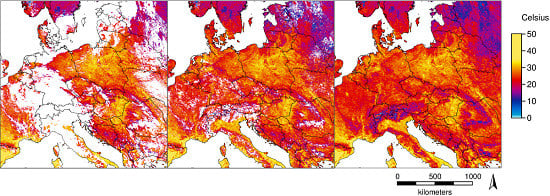
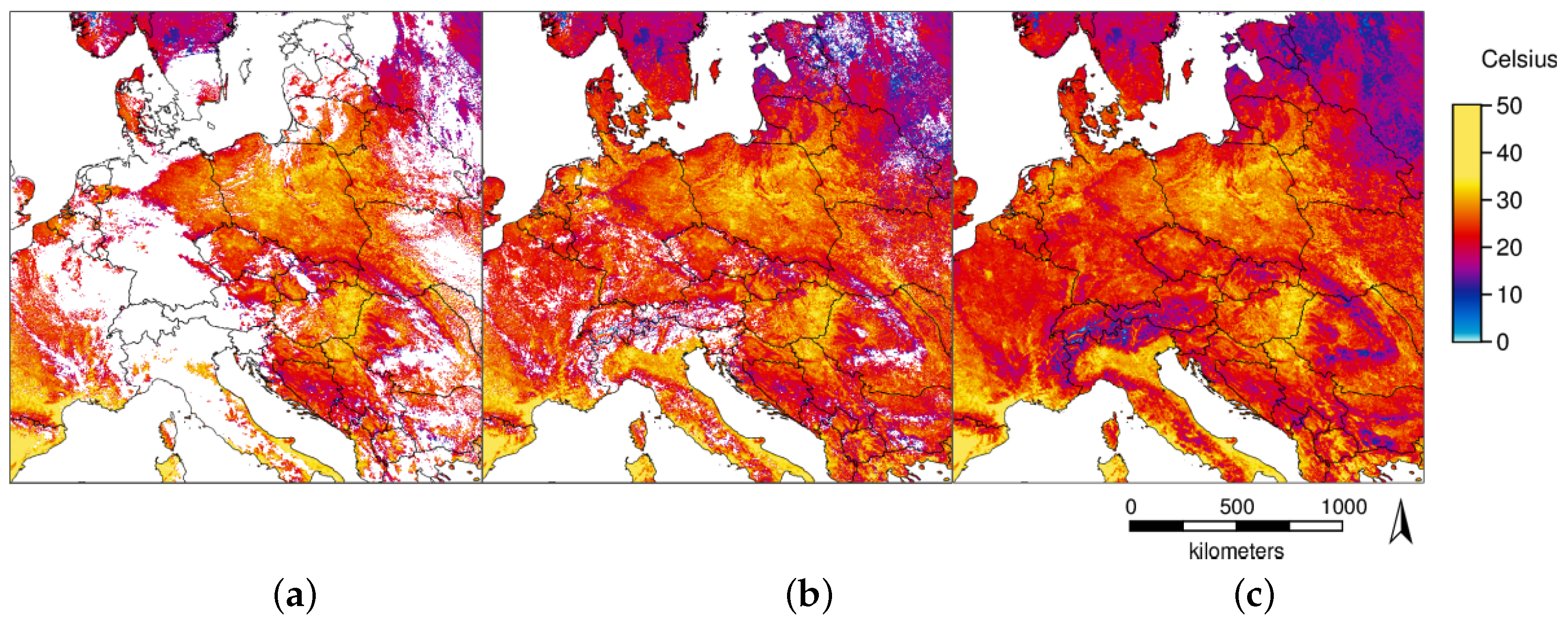
Reconstruction of missing values for 8 June 2016: (a) original LST data; (b) after temporal interpolation; and (c) after spatial interpolation.
Figure 4.
Reconstruction of missing values for 8 June 2016: (a) original LST data; (b) after temporal interpolation; and (c) after spatial interpolation.

Figure 5.
Spatial distribution of the percentage of LST outliers aggregated over the years 2003 to 2016 for the months January, April, July, and October.
Figure 5.
Spatial distribution of the percentage of LST outliers aggregated over the years 2003 to 2016 for the months January, April, July, and October.

Figure 6.
Percentage of LST outliers aggregated for each overpass time of day over all days and years: (a) at 01:30, 6.1% outliers; and (b) at 13:30, 5.7% outliers.
Figure 6.
Percentage of LST outliers aggregated for each overpass time of day over all days and years: (a) at 01:30, 6.1% outliers; and (b) at 13:30, 5.7% outliers.

Figure 7.
Results of LST reconstruction for January 2015: (a) with emissivity as additional variable; (b) without emissivity (c.f, old “EuroLST” from [5]); and (c) corresponding land cover types. The displayed area covers Switzerland and parts of France and Germany. The slightly higher temperatures of urban areas are represented, and water bodies are more clearly delineated when considering emissivity.

Figure 8.
Comparison of monthly averages for 2003 for Bonn, Germany from the new LST reconstruction (LST), the old LST reconstruction (“EuroLST” data, [5]), the original LST values of the MODIS 11A1 products (LST_raw), and air temperature from ground station records from the German Weather Service (DWD).

Figure 9.
LST time series for Bonn, Germany, in December 2016, for central Europe (black) and globally (red) with: (a) original LST values; and (b) reconstructed LST values. Time steps per day correspond to MODIS overpass times: 01:30, 10:30, 13:30 and 22:30.
Figure 9.
LST time series for Bonn, Germany, in December 2016, for central Europe (black) and globally (red) with: (a) original LST values; and (b) reconstructed LST values. Time steps per day correspond to MODIS overpass times: 01:30, 10:30, 13:30 and 22:30.

Figure 10.
Intensity of the heat wave in Europe in August 2003 expressed as number of standard deviations away from the average temperature in August. Global heat wave analysis based on MOD11C1/MYD11C1 is shown in (a); and zoomed to Europe in (b). The equivalent higher resolution result based on MOD11A1/MYD11A1 is shown in (c).

Figure 11.
Comparison of January and July 2016 LST to the reference time series given as numbers of standard deviations from the long term average (intensity) and as corresponding quantiles of the reference time series (rarity).
Figure 11.
Comparison of January and July 2016 LST to the reference time series given as numbers of standard deviations from the long term average (intensity) and as corresponding quantiles of the reference time series (rarity).


Table 1.
Difference of the reconstruction over simulated gaps with the raw data in K. For reference, the difference of the reconstructed land surface temperature (LST) values without simulation (only outlier filtering) to the raw data is also provided.
Table 1.
Difference of the reconstruction over simulated gaps with the raw data in K. For reference, the difference of the reconstructed land surface temperature (LST) values without simulation (only outlier filtering) to the raw data is also provided.
| Hole Size in Pixels | Simulation-Raw LST | Reconstructed-Raw LST |
|---|---|---|
| 9 | −1.17 | −0.42 |
| 61 | −1.91 | −0.07 |
| 161 | −2.44 | −0.07 |
| 305 | −2.57 | 0.03 |
| 509 | −2.63 | 0.01 |
| 761 | −2.61 | 0.03 |
| 1069 | −2.65 | 0.02 |
| 1425 | −2.73 | 0.01 |
Table 2.
Calibration of reconstructed monthly MODIS LST data for 2016 against air temperature data of meteorological stations from the German Weather Service (DWD) and elevation. Values in brackets are the results without elevation as additional explanatory variable. AIC: Akaike information criterion; RMSE: root mean square error.
| Month | n Stations | R2 | AIC | RMSE |
|---|---|---|---|---|
| Jan | 486 | 0.85 (0.83) | −433.2 (−379.1) | 0.64 (0.67) |
| Feb | 487 | 0.86 (0.82) | −690.6 (−554.8) | 0.49 (0.56) |
| Mar | 487 | 0.90 (0.84) | −795.2 (−580.6) | 0.44 (0.55) |
| Apr | 484 | 0.85 (0.62) | −688.4 (−231.6) | 0.49 (0.78) |
| May | 484 | 0.91 (0.72) | −732.7 (−193.7) | 0.47 (0.82) |
| Jun | 483 | 0.89 (0.74) | −698.7 (−302.2) | 0.48 (0.73) |
| Jul | 484 | 0.86 (0.67) | −643.2 (−220.3) | 0.51 (0.79) |
| Aug | 486 | 0.84 (0.69) | −656.9 (−330.2) | 0.51 (0.71) |
| Sep | 489 | 0.86 (0.61) | −685.2 (−207.1) | 0.49 (0.81) |
| Oct | 485 | 0.90 (0.52) | −937.0 (−183.0) | 0.38 (0.82) |
| Nov | 489 | 0.83 (0.79) | −701.9 (−594.9) | 0.48 (0.54) |
| Dec | 486 | 0.71 (0.40) | −91.3 (258.7) | 0.90 (1.30) |
© 2017 by the authors. Licensee MDPI, Basel, Switzerland. This article is an open access article distributed under the terms and conditions of the Creative Commons Attribution (CC BY) license (http://creativecommons.org/licenses/by/4.0/).
Share and Cite
MDPI and ACS Style
Metz, M.; Andreo, V.; Neteler, M. A New Fully Gap-Free Time Series of Land Surface Temperature from MODIS LST Data. Remote Sens. 2017, 9, 1333. https://0-doi-org.brum.beds.ac.uk/10.3390/rs9121333
AMA Style
Metz M, Andreo V, Neteler M. A New Fully Gap-Free Time Series of Land Surface Temperature from MODIS LST Data. Remote Sensing. 2017; 9(12):1333. https://0-doi-org.brum.beds.ac.uk/10.3390/rs9121333
Chicago/Turabian StyleMetz, Markus, Verónica Andreo, and Markus Neteler. 2017. "A New Fully Gap-Free Time Series of Land Surface Temperature from MODIS LST Data" Remote Sensing 9, no. 12: 1333. https://0-doi-org.brum.beds.ac.uk/10.3390/rs9121333
Note that from the first issue of 2016, this journal uses article numbers instead of page numbers. See further details here.