
AF-DHNN: Fuzzy Clustering and Inference-Based Node Fault Diagnosis Method for Fire Detection


Abstract
:1. Introduction
2. Related Works
2.1. The Diagnostic Methods Based on Traditional Probability Theory
2.2. Distributed Fault Detection Methods
2.3. The Diagnosis Method Based on Artificial Intelligence
2.4. Other Diagnostic Methods
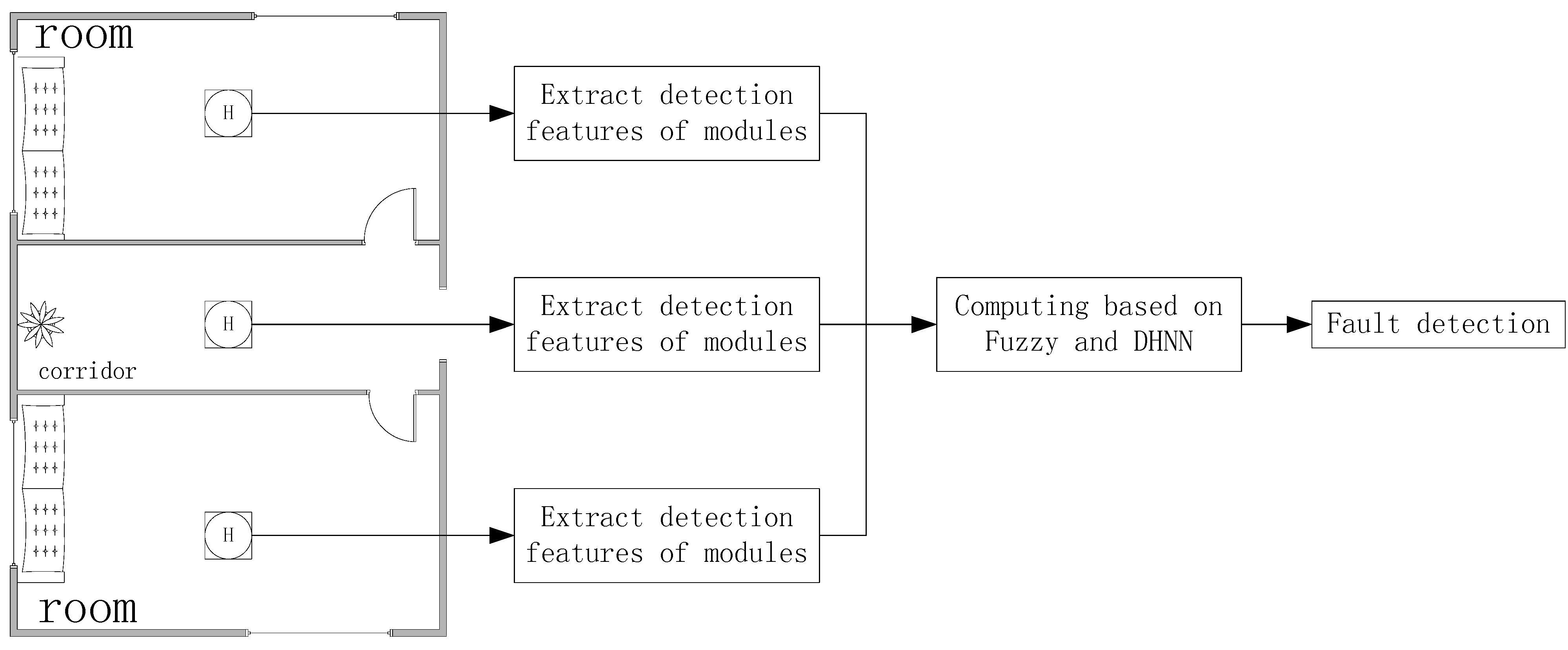
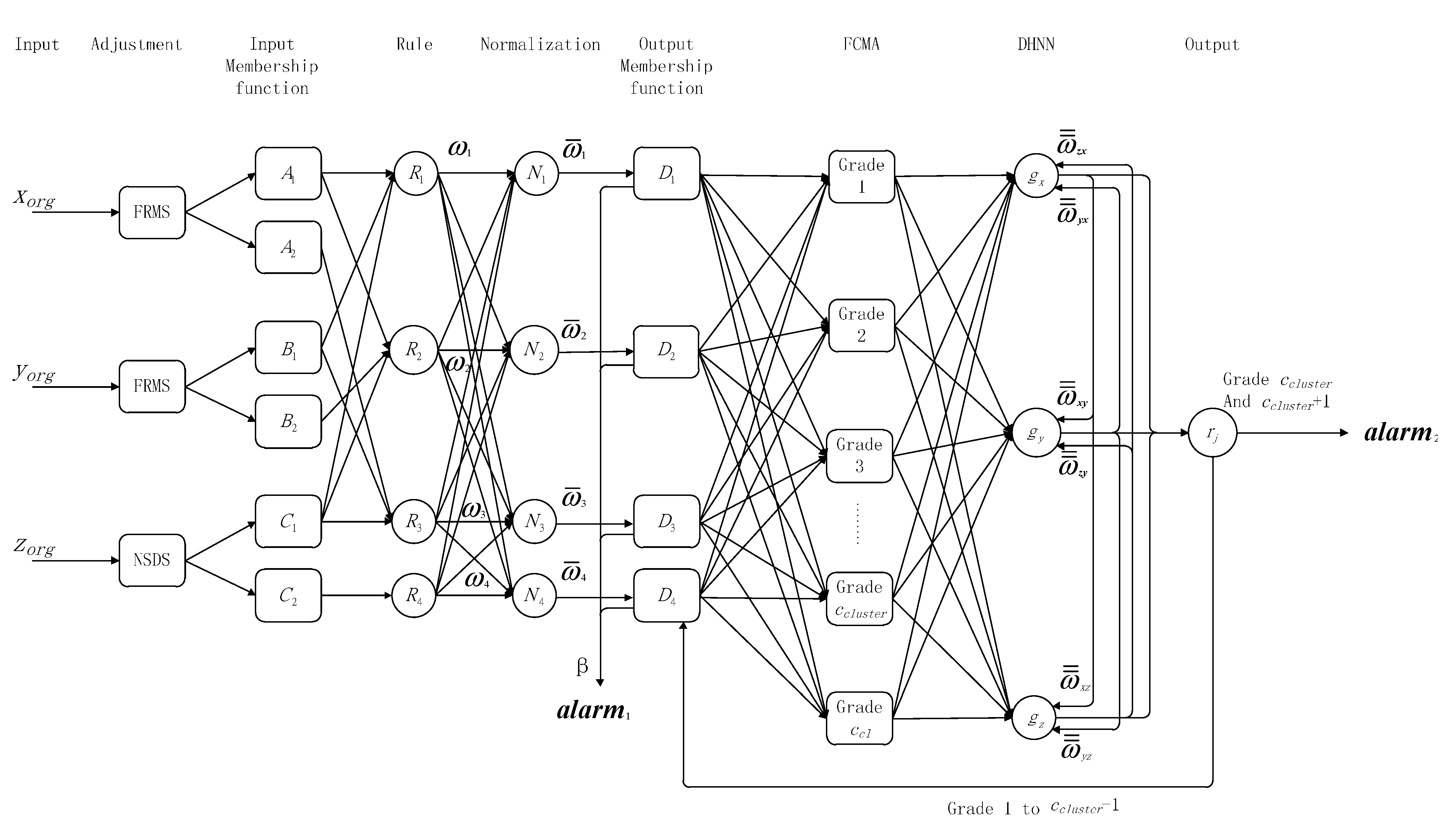
3. The Method Based on AF-DHNN

3.1. Selection of Two Features for Detected Signals
3.1.1. FRMS
3.1.2. NSDS
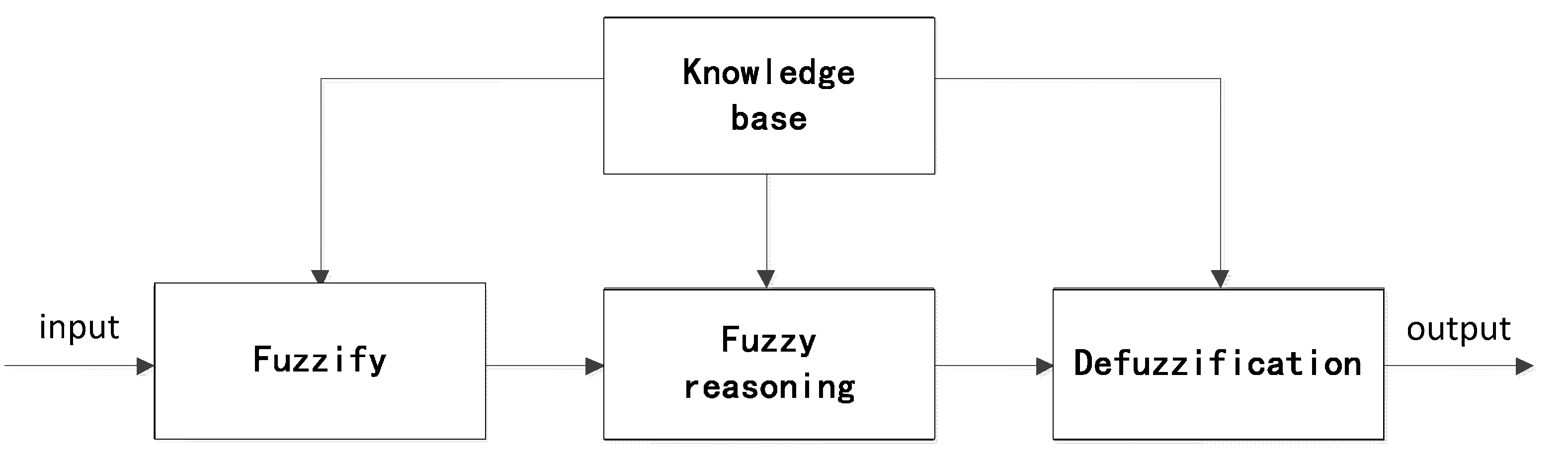
3.2. Fuzzy Inference Operator

3.2.1. Basic Design

| Output State | Flue Gas Dimming Extent | Ambient Temperature | Communication Module | Node State |
|---|---|---|---|---|
| normal | A1 | B1 | C1 | D1 |
| abnormal | A2 | B2 | C2 | D2, D3, D4 |
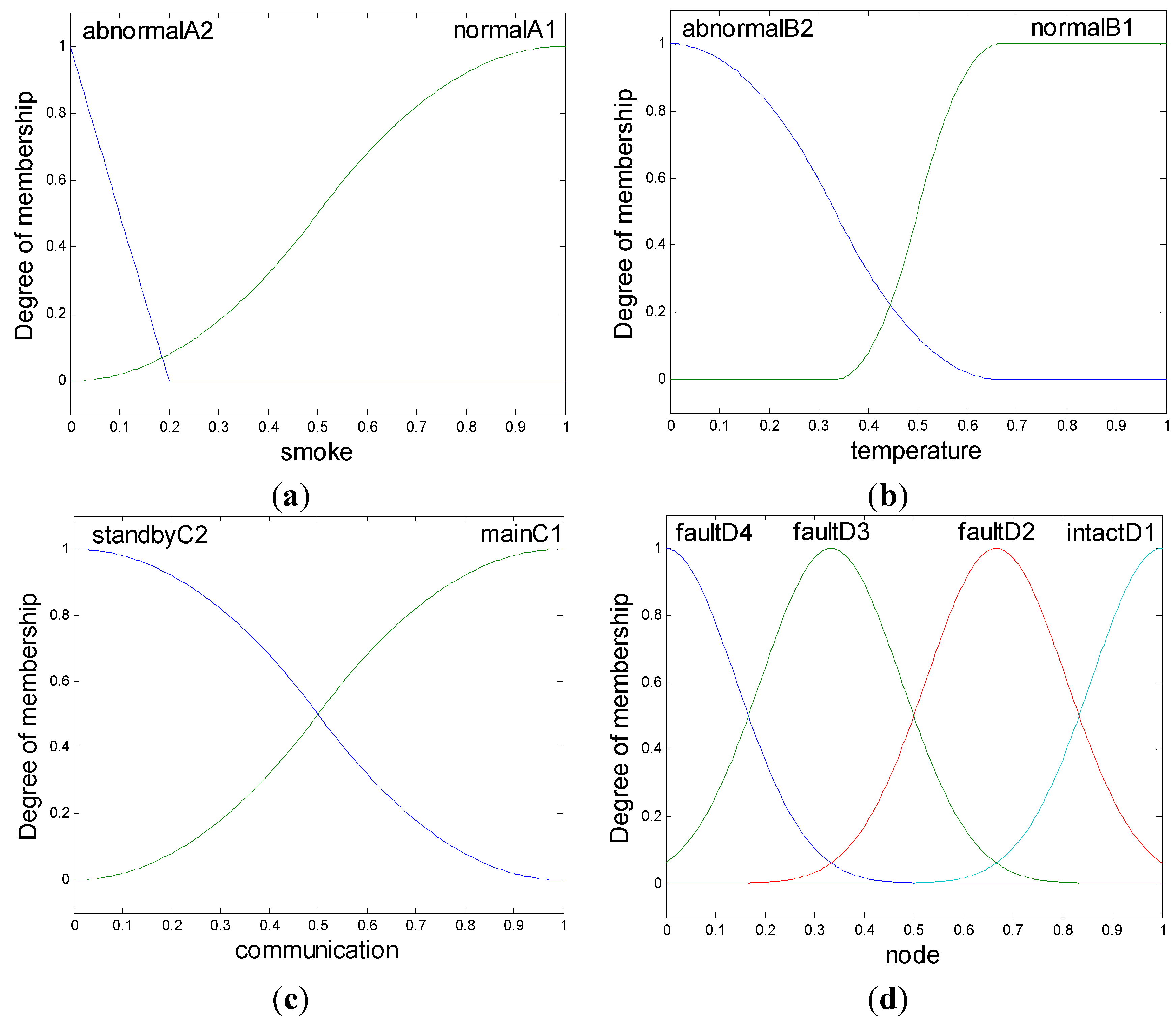
- A1——Smoke sensing module is normal;
- A2——Smoke sensing module is abnormal;
- B1——Temperature sensing module is normal;
- B2——Temperature sensing module is abnormal;
- C1——Enable the main communication module;
- C2——Enable the standby communication module;
- D1——Overall state of node is normal;
- D2——Smoke sensing module fault;
- D3——Temperature sensing module fault;
- D4——Node main communication module fault, switching to standby communication module.
3.2.2. Membership Function and Rules

- R1: IF x is A1 and y is B1 and z is C1 THEN s is D1
- R2: IF x is A1 and y is B1 and z is C1 THEN s is D2
- R3: IF x is A2 and y is B1 and z is C1 THEN s is D3
- R4: IF z is C2 THEN s is D4

3.2.3. Normalization
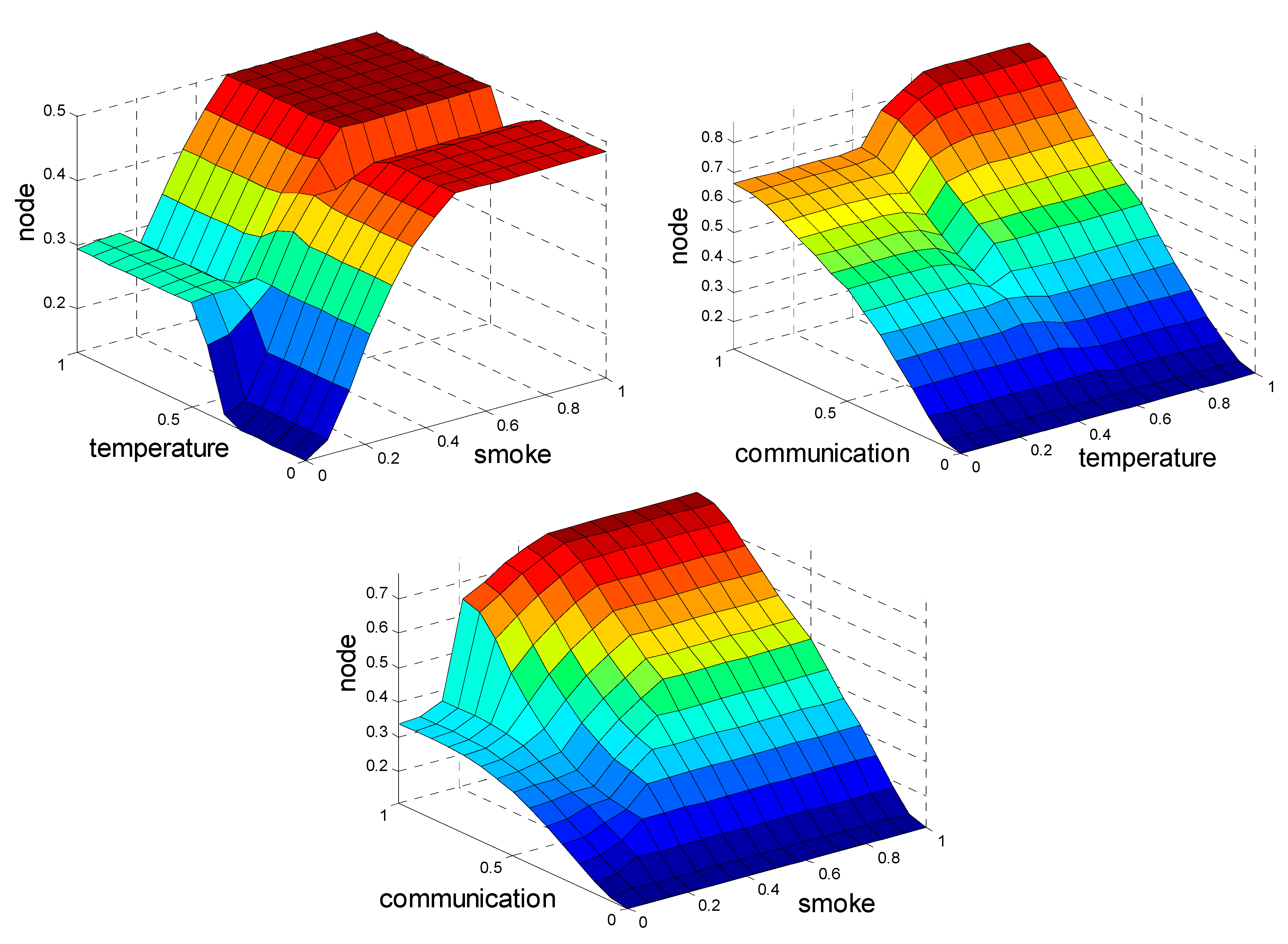
3.2.4. Output Membership Function
3.3. FCMA Operator
| Algorithm 1. Sorting and classification algorithm. | |
| Inputs: Si, j, i = 1, 2, … n, j = 1, 2, … ccl E = {eγi} Outputs: Refresh Si, j, O1 Initialize: i, j | |
| 1. | Si, j = , i = 1, 2, … n, j = 1, 2, … ccl |
| 2. | Establish grades standard: |
| 3. | |
| 4. | |
| 5. | |
| 6. | Classified the data: |
| 7. | For 1 ≤ j ≤ ccl; For 1 ≤ i ≤ n |
| 8. | |
| 9. | |
3.4. Discrete Hopfield Network

3.5. Output and Feedback
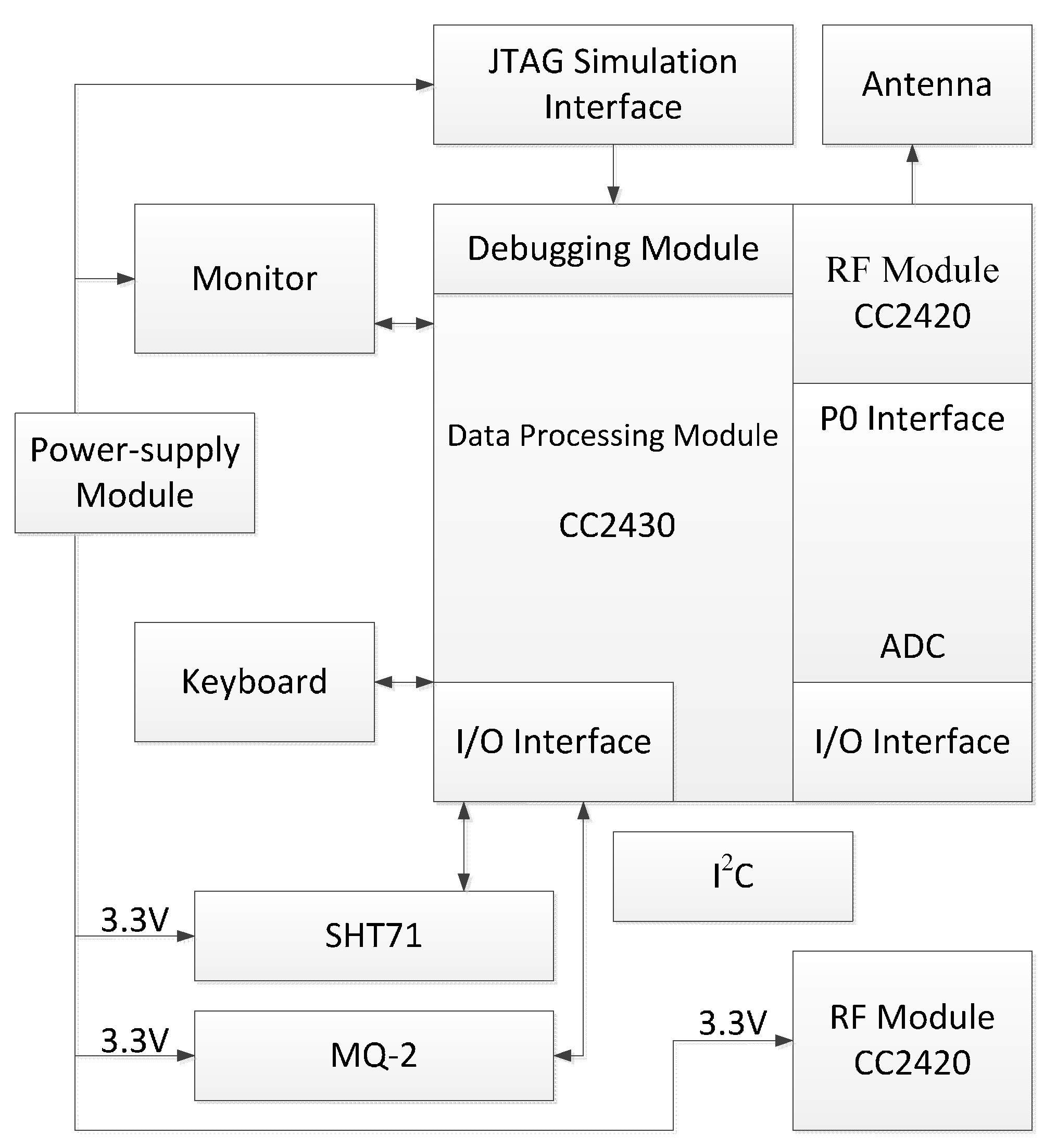
3.6. Implementation of the Algorithm

4. Simulation and Analysis Results
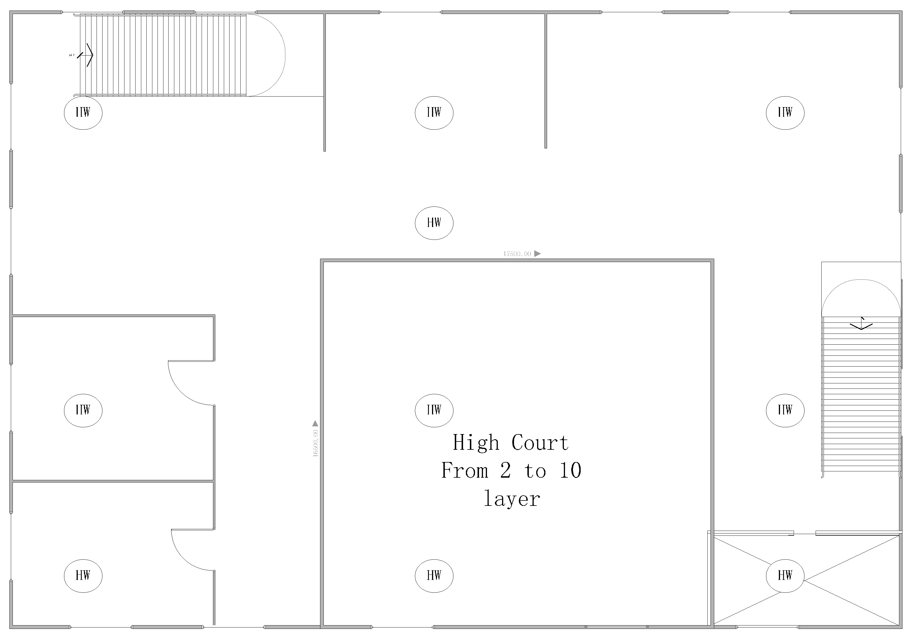
4.1. Network Structure
4.2. Sample Parameters
 stands the vertical position of sensor nodes on each layer.


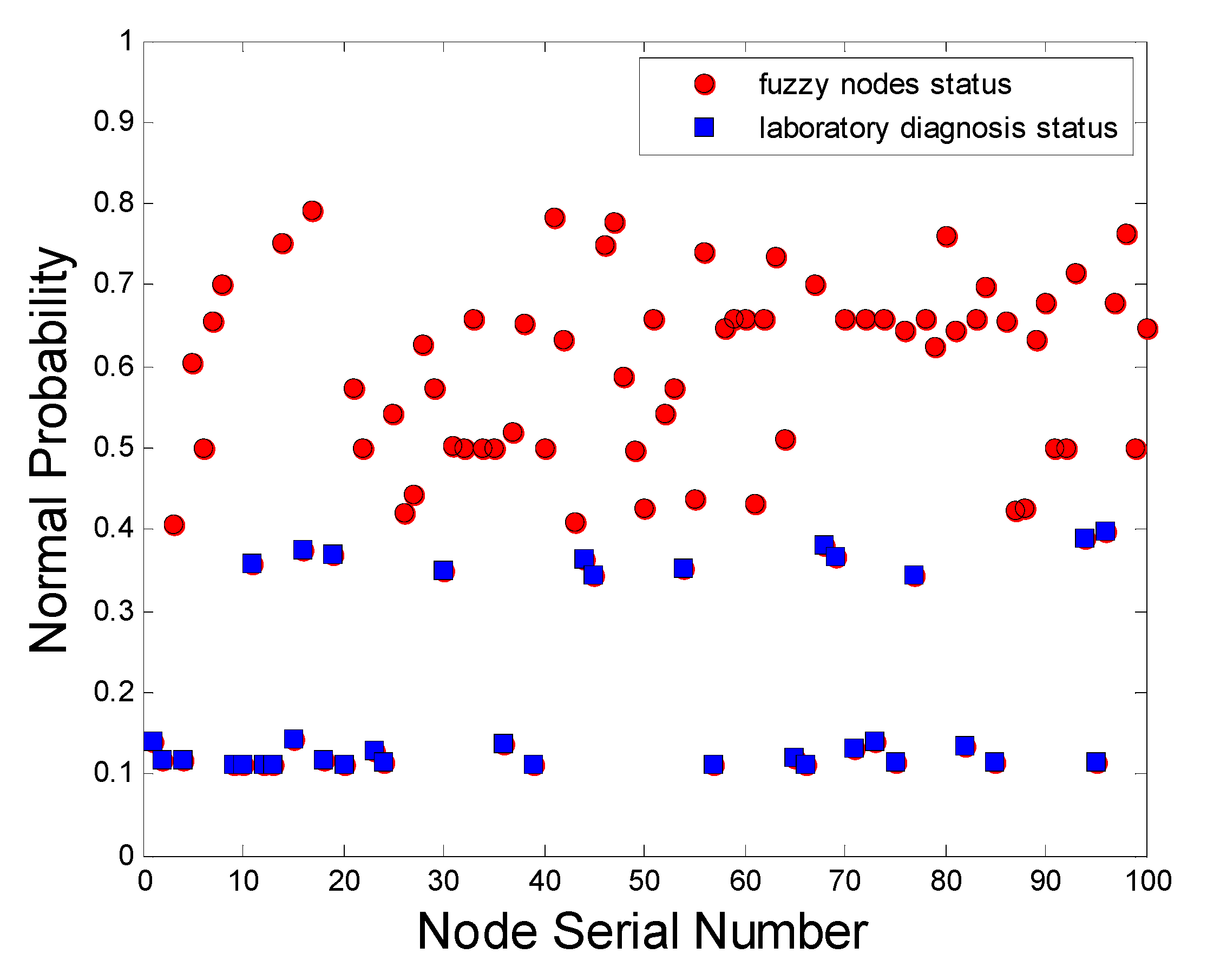
4.3. Conclusion Analysis
4.3.1. Fuzzy Input


- ;
- ;
- ;
- .
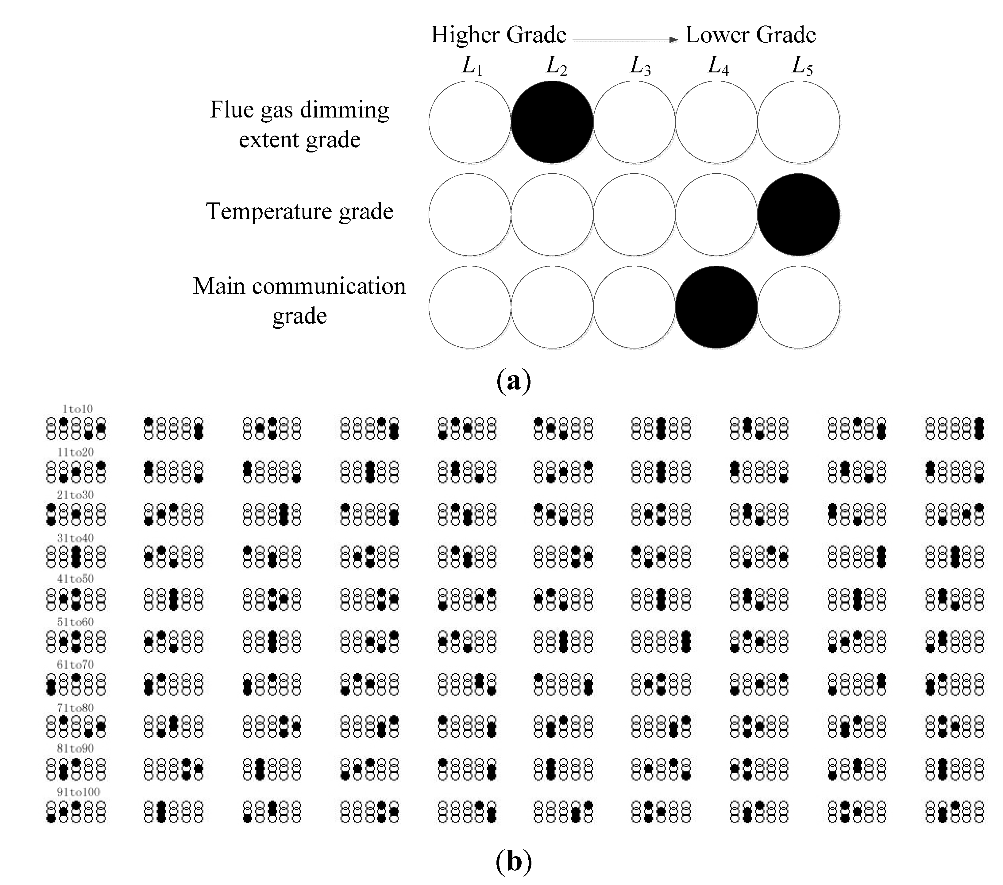
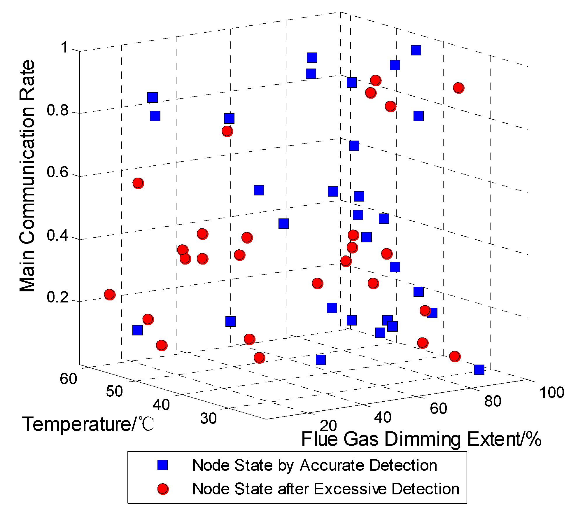
4.3.2. Diagnostic Method Performance Comparison
| Grade | Flue Gas Dimming Extent Grade | Flue Gas Dimming Extent | Temperature Grade | Temperature | Main Communication Grade | Main Communication |
|---|---|---|---|---|---|---|
| L1 | 0.9482 | 0.9482 | 0.9845 | |||
| L2 | 0.7898 | 0.7897 | 0.9018 | |||
| L3 | 0.5516 | 0.3192 | 0.5973 | |||
| L4 | 0.1680 | 0.3143 | 0.0607 | |||
| L5 | 0 | 0 | 0 |

| Grade | Flue Gas Dimming Extent Grade | Flue Gas Dimming Extent | Temperature Grade | Temperature | Main Communication Grade | Main Communication |
|---|---|---|---|---|---|---|
| L1 | 15 | 15 | 20 | |||
| L2 | 29 | 29 | 20 | |||
| L3 | 34 | 31 | 31 | |||
| L4 | 10 | 6 | 13 | |||
| L5 | 12 | 19 | 16 |

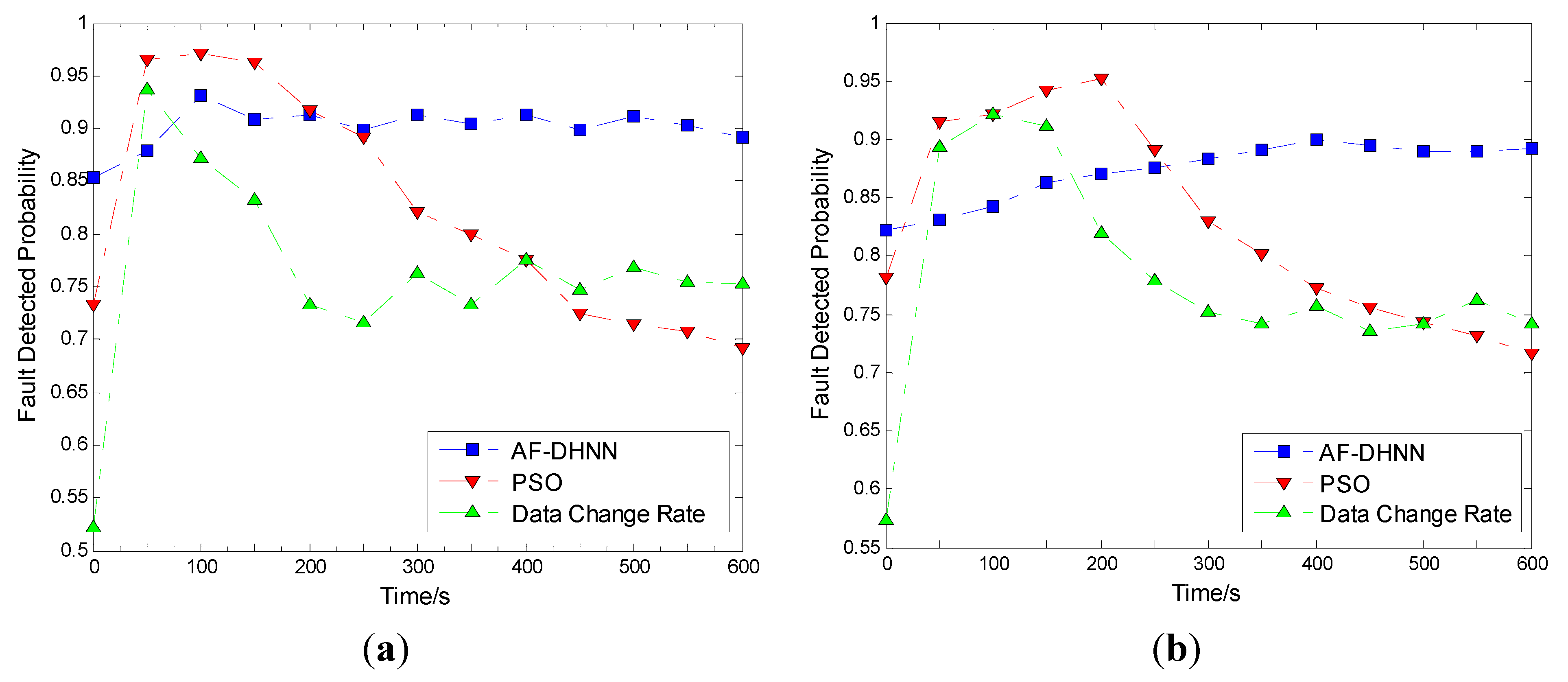
| Project | The Actual Number of Failure | AF-DHNN | Data Change Rate | PSO | ||||||
|---|---|---|---|---|---|---|---|---|---|---|
| The Accuracy Rate of Diagnosis | Maintenance Number (Piece) | The Time of Diagnosis (s) | The Accuracy Rate of Diagnosis | Maintenance Number (Piece) | The Time of Diagnosis (s) | The Accuracy Rate of Diagnosis | Maintenance Number (Piece) | The Time of Diagnosis (s) | ||
| Photoelectric smoke module | 20 | 100% | 22 | 10 | 80% | 28 | 100 | 85% | 32 | 10 |
| Temperature sensing module | 23 | 95.65% | 25 | 10 | 73.91% | 44 | 100 | 86.95% | 47 | 10 |
| The main communication module | 26 | 100% | 29 | 10 | 76.92% | 32 | 100 | 76.92% | 35 | 10 |
| Node | 35 | 97.14% | 40 | 13.3 | 77.14% | 53 | 124.2 | 82.85% | 55 | 15.7 |


4.3.3. Performance Comparison in a Fire


5. Conclusions
Acknowledgments
Author Contributions
Conflicts of Interest
References
- Estima, J.O.; Marques, C.; Antonio, J. A New Algorithm for Real-Time Multiple Open-Circuit Fault Diagnosis in Voltage-Fed PWM Motor Drives by the Reference Current Errors. IEEE Trans. Ind. Electron. 2013, 42, 3496–3505. [Google Scholar] [CrossRef]
- Torkaman, H.; Afjei, E.; Yadegari, P. Static, Dynamic, and Mixed Eccentricity Faults Diagnosis in Switched Reluctance Motors Using Transient Finite Element Method and Experiments. IEEE Trans. Mag. 2012, 48, 2254–2264. [Google Scholar] [CrossRef]
- Seera, M.; Lim, C.P.; Ishak, D.; Ishak, D.; Singh, H. Fault Detection and Diagnosis of Induction Motors Using Motor Current Signature Analysis and a Hybrid FMM-CART Model. IEEE Trans. Neural Netw. Learn. Syst. 2012, 23, 97–108. [Google Scholar] [CrossRef] [PubMed]
- Freire, N.M.A.; Estima, J.O.; Marques, C.A.J. Open-Circuit Fault Diagnosis in PMSG Drives for Wind Turbine Applications. IEEE Trans. Ind. Electron. 2013, 60, 3957–3967. [Google Scholar] [CrossRef]
- Mirzaee, A.; Salahshoor, K. Fault diagnosis and accommodation of nonlinear systems based on multiple-model adaptive unscented Kalman filter and switched MPC and H-infinity loop-shaping controller. J. Process Control 2012, 22, 626–634. [Google Scholar] [CrossRef]
- Villa, L.F.; Renones, A; Peran, J.R.; de Miguel, L.J. Statistical fault diagnosis based on vibration analysis for gear test-bench under non-stationary conditions of speed and load. Mech. Syst. Signal Proc. 2012, 29, 436–446. [Google Scholar] [CrossRef]
- Lemos, A.; Caminhas, W.; Gomide, F. Adaptive fault detection and diagnosis using an evolving fuzzy classifier. Inform. Sci. 2013, 220, 64–85. [Google Scholar] [CrossRef]
- Brunson, C.; Empringham, L.; de Lillo, L.; Wheeler, P.; Clare, J. Open-Circuit Fault Detection and Diagnosis in Matrix Converters. IEEE Trans. Power Electron. 2015, 30, 2840–2847. [Google Scholar] [CrossRef]
- Nembhard, A.D.; Sinha, J.K.; Yunusa-Kaltungo, A. Development of a generic rotating machinery fault diagnosis approach insensitive to machine speed and support type. J. Sound Vib. 2015, 337, 321–341. [Google Scholar] [CrossRef]
- Perdomo-Ortiz, A.; Fluegemann, J.; Narasimhan, S.; Biswas, R.; Smelyanskiy, V.N. A quantum annealing approach for fault detection and diagnosis of graph-based systems. Eur. Phys. J.-Spec. Top. 2015, 224, 131–148. [Google Scholar] [CrossRef]
- Panda, M.; Khilar, P.M. Distributed self-fault diagnosis algorithm for large scale wireless sensor networks using modified three sigma edit test. Ad. Hoc. Netw. 2015, 25, 170–184. [Google Scholar] [CrossRef]
- Chabir, K.; Sid, M.A.; Sauter, D. Fault Diagnosis in a Networked Control System under Communication Constraints: A Quadrotor Application. Int. J. Appl. Math. Comput. Sci. 2014, 24, 809–820. [Google Scholar] [CrossRef]
- Seron, M.M.; de Dona, J.A.; Richter, J.H. Invariant-set-based fault diagnosis in Lure systems. Int. J. Robust Nonlinear Control 2014, 24, 2405–2422. [Google Scholar] [CrossRef]
- Zhao, B.; Skjetne, R.; Blanke, M.; Dukan, F. Particle Filter for Fault Diagnosis and Robust Navigation of Underwater Robot. IEEE Trans. Control Syst. Technol. 2014, 22, 2399–2407. [Google Scholar] [CrossRef] [Green Version]
- Shahriari-kahkeshi, M.; Sheikholeslam, F. Adaptive fuzzy wavelet network for robust fault detection and diagnosis in non-linear systems. IET Control Theory Appl. 2014, 8, 1487–1498. [Google Scholar] [CrossRef]
- Lefebvre, D. Fault Diagnosis and Prognosis with Partially Observed Petri Nets. IEEE Trans. Syst. Man Cybern.-Syst. 2014, 44, 1413–1424. [Google Scholar] [CrossRef]
- Ghanbari, T.; Farjah, A. A Magnetic Leakage Flux-Based Approach for Fault Diagnosis in Electrical Machines. IEEE Sens. J. 2014, 14, 2981–2988. [Google Scholar] [CrossRef]
- Talhaoui, H.; Menacer, A.; Kessal, A.; Kechida, R. Fast Fourier and discrete wavelet transforms applied to sensorless vector control induction motor for rotor bar faults diagnosis. ISA Trans. 2014, 53, 1639–1649. [Google Scholar] [CrossRef] [PubMed]
- Hernandez, H.R.; Camas, J.L.; Medina, A.; Perez, M.; le Lann, M.V. Fault Diagnosis by LAMDA Methodology Applied to Drinking Water Plant. IEEE Latin Am. Trans. 2014, 12, 985–990. [Google Scholar] [CrossRef]
- Sahoo, M.N.; Khilar, P.M. Diagnosis of Wireless Sensor Networks in Presence of Permanent and Intermittent Faults. Wirel. Pers. Commun. 2014, 78, 1571–1591. [Google Scholar] [CrossRef]
- Zhou, F.Q.; Su, Z.; Chai, X.H.; Chen, L.P. Detection of foreign matter in transfusion solution based on Gaussian background modeling and an optimized BP neural network. Sensors 2014, 14, 19945–19962. [Google Scholar] [CrossRef] [PubMed]
- Que, R.Y.; Zhu, R. Aircraft aerodynamic parameter detection using micro hot-film flow sensor array and BP neural network identification. Sensors 2012, 12, 10920–10929. [Google Scholar] [CrossRef] [PubMed]
- Han, J.; Chang, H.; Yang, Q.; Fontenay, G.; Groesser, T.; Barcellos-Hoff, M.H.; Parvin, B. Multiscale iterative voting for differential analysis of stress response for 2D and 3D cell culture models. J. Microsc. 2011, 241, 315–326. [Google Scholar] [CrossRef] [PubMed]
- De Luis Balaguer, M.A.; Williams, C.M. Hierarchical modularization of biochemical pathways using fuzzy-c means clustering. IEEE Trans. Cybern. 2014, 44, 1473–1484. [Google Scholar] [CrossRef] [PubMed]
- Hemanth, D.J.; Vijila, C.K.; Selvakumar, A.I.; Antitha, J. Performance Improved Iteration-Free Artificial Neural Networks for Abnormal Magnetic Resonance Brain Image Classification. Neurocomputing 2014, 130, 98–107. [Google Scholar] [CrossRef]
- Modares, H.; Lewis, F.L.; Naghibi-Sistani, M. Adaptive Optimal Control of Unknown Constrained-Input Systems Using Policy Iteration and Neural Networks. IEEE Trans. Neural Netw. Learn. Syst. 2013, 24, 1513–1525. [Google Scholar] [CrossRef] [PubMed]
- Abin, A.A.; Beigy, H. Active constrained fuzzy clustering: A multiple kernels learning approach. Pattern Recognit. 2015, 48, 953–967. [Google Scholar] [CrossRef]
- Zolkepli, M.; Dong, F.Y.; Hirota, K. Automatic Switching of Clustering Methods based on Fuzzy Inference in Bibliographic Big Data Retrieval System. Int. J. Fuzzy Log. Intell. Syst. 2015, 14, 256–267. [Google Scholar] [CrossRef]
- Oussalah, M.; Alakhras, M.; Hussein, M.I. Multivariable fuzzy inference system for fingerprinting indoor localization. Fuzzy Sets Syst. 2015, 269, 65–89. [Google Scholar] [CrossRef]
- Hajihassani, M.; Marto, A.; Khezri, N. Indirect measure of thermal conductivity of rocks through adaptive neuro-fuzzy inference system and multivariate regression analysis. Measurement 2015, 67, 71–77. [Google Scholar] [CrossRef]
- Sert, S.A.; Bagci, H.; Yazici, A. MOFCA: Multi-objective fuzzy clustering algorithm for wireless sensor networks. Appl. Soft Comput. 2015, 30, 151–165. [Google Scholar] [CrossRef]
- Nguyen, T.T.; Le, H.S. HIFCF: An effective hybrid model between picture fuzzy clustering and intuitionistic fuzzy recommender systems for medical diagnosis. Expert Syst. Appl. 2013, 42, 3682–3701. [Google Scholar]
- Safizadeh, M.S.; Latifi, S.K. Using multi-sensor data fusion for vibration fault diagnosis of rolling element bearings by accelerometer and load cell. Inform. Fusion 2014, 18, 1–8. [Google Scholar] [CrossRef]
- Hamidreza, M.; Mehdi, S.; Hooshang, J.R.; Aliakbar, N. Reconstruction based approach to sensor fault diagnosis using auto-associative neural networks. J. Central South Univ. 2014, 21, 2273–2281. [Google Scholar] [CrossRef]
- Alippi, C.; Roveri, M.; Trovo, F. A Self-Building and Cluster-Based Cognitive Fault Diagnosis System for Sensor Networks. IEEE Trans. Neural Netw. Learn. Syst. 2014, 25, 1021–1032. [Google Scholar]
- Tadic, P.; Durovic, Z. Particle filtering for sensor fault diagnosis and identification in nonlinear plants. J. Process Control 2014, 24, 401–409. [Google Scholar] [CrossRef]
- Park, J.H.; Kang, H.C.; Jung, D.H. Level-Converting Retention Flip-Flop for Reducing Standby Power in ZigBee SoCs. IEEE Trans. Very Large Scale Integr. Syst. 2015, 23, 413–421. [Google Scholar] [CrossRef]
- Shariff, F.; Abd Rahim, N.; Ping, H.W. Zigbee-based data acquisition system for online monitoring of grid-connected photovoltaic system. Expert Syst. Appl. 2015, 42, 1730–1742. [Google Scholar] [CrossRef]
- Oliva, P.; Schroeder, W. Assessment of VIIRS 375 m active fire detection product for direct burned area mapping. Remote Sens. Environ. 2015, 160, 144–155. [Google Scholar] [CrossRef]
- Arnett, J.T.T.R.; Coops, N.C.; Daniels, L.D.; Falls, R.W. Detecting forest damage after a low-severity fire using remote sensing at multiple scales. Int. J. Appl. Earth Obs. Geoinform. 2015, 35, 239–246. [Google Scholar] [CrossRef]
- Demetgul, M.; Yildiz, K.; Taskin, S.; Tansel, I.N.; Yazicioglu, O. Fault diagnosis on material handling system using feature selection and data mining techniques. Measurement 2014, 55, 15–24. [Google Scholar] [CrossRef]
- Demetgul, M.; Yazicioglu, O.; Kentli, A. Radial Basis and LVQ Neural Network Algorithm for Real Time Fault Diagnosis of Bottle Filling Plant. Tehnicki Vjesnik-Technical Gazette 2014, 21, 689–695. [Google Scholar]
- Rahme, S.; Meskin, N. Adaptive sliding mode observer for sensor fault diagnosis of an industrial gas turbine. Control Eng. Pract. 2015, 38, 57–74. [Google Scholar] [CrossRef]
- Funano, S.; Sugahara, M.; Henares, T.G.; Sueyoshi, K.; Endo, T.; Hisamoto, H. A single-step enzyme immunoassay capillary sensor composed of functional multilayer coatings for the diagnosis of marker proteins. Analyst 2015, 140, 1459–1465. [Google Scholar] [CrossRef] [PubMed]
- Lefebvre, D. Fault diagnosis and prognosis with partially observed stochastic Petri nets. Proc. Instit. Mech. Eng. Part O-J. Risk Reliab. 2014, 228, 382–396. [Google Scholar] [CrossRef]
- Hussain, S.; Mokhtar, M.; Howe, J.M. Sensor Failure Detection, Identification, and Accommodation Using Fully Connected Cascade Neural Network. IEEE Trans. Ind. Electron. 2015, 62, 1683–1692. [Google Scholar] [CrossRef]
- Gonzale, R.; Huang, B. Control loop diagnosis with ambiguous historical operating modes: Part 2, information synthesis based on proportional parametrization. J. Process Control 2013, 23, 1441–1454. [Google Scholar] [CrossRef]
- Lauenroth, A.; Knipping, S.; Schwesig, R. Vestibular disorders. Effects of sensorimotor training on postural regulation and on recovery process. HNO 2012, 60, 692–699. [Google Scholar] [CrossRef] [PubMed]
- Zhu, Y.H.; Jin, X.Q.; Du, Z.M. Fault diagnosis for sensors in air handling unit based on neural network pre-processed by wavelet and fractal. Energy Build. 2013, 44, 7–16. [Google Scholar] [CrossRef]
- Li, X.M.; Yang, Y.; Hou, Y.; Yang, J.T.; Qin, B.G.; Fu, G.; Gu, L.Q. Diagnostic Accuracy of Three Sensory Tests for Diagnosis of Sensory Disturbances. J. Reconstr. Microsurg. 2015, 31, 67–73. [Google Scholar] [CrossRef] [PubMed]
- Martin, A.; Batalla, P.; Hernandez-Ferrer, J.; Martinez, M.T.; Escarpa, A. Graphene oxide nanoribbon-based sensors for the simultaneous bio-electrochemical enantiomeric resolution and analysis of amino acid biomarkers. Biosens. Bioelectron. 2015, 68, 163–167. [Google Scholar] [CrossRef] [PubMed]
- Abdulghani, A.H.; Prakash, S.; Ali, M.Y.; Deeth, H.C. Sensory evaluation and storage stability of UHT milk fortified with iron, magnesium and zinc. Dairy Sci. Technol. 2015, 95, 33–46. [Google Scholar] [CrossRef]
- Bhowmik, B.; Hazra, A.; Dutta, K. Repeatability and Stability of Room-Temperature Acetone Sensor Based on TiO2 Nanotubes: Influence of Stoichiometry Variation. IEEE Trans. Device Mater. Reliab. 2014, 14, 961–967. [Google Scholar] [CrossRef]
- Wan, K.T.; Leung, C.K.Y. Durability Tests of a Fiber Optic Corrosion Sensor. Sensors 2012, 12, 3656–3668. [Google Scholar] [CrossRef] [PubMed]
- Kang, D.; Pikhitsa, P.V.; Choi, Y.W. Ultrasensitive mechanical crack-based sensor inspired by the spider sensory system. Nature 2014, 516, 222–226. [Google Scholar] [CrossRef] [PubMed]
- Demetgul, M.; Yazicioglu, O.; Kentli, A. Radial basis and lvq neural network algorithm for real time fault diagnosis of bottle filling plant. Tehnicki Vjesnik-Technical Gazette 2014, 21, 689–695. [Google Scholar]
- Hu, Y.F.; Ding, Y.S.; Ren, L.H.; Hao, K.R.; Han, H. An endocrine cooperative particle swarm optimization algorithm for routing recovery problem of wireless sensor networks with multiple mobile sinks. Inform. Sci. 2015, 300, 100–113. [Google Scholar] [CrossRef]
- Quevedo, J.; Chen, H.; Cuguero, M.A.; Tino, P.; Puig, V.; Garcia, D.; Sarrate, R.; Yao, X. Combining learning in model space fault diagnosis with data validation/reconstruction: Application to the Barcelona water network. Eng. Appl. Artif. Intell. 2014, 30, 18–29. [Google Scholar] [CrossRef]
- Potamianos, P.G.; Mitronikas, E.D.; Safacas, A.N. Open-Circuit Fault Diagnosis for Matrix Converter Drives and Remedial Operation Using Carrier-Based Modulation Methods. IEEE Trans. Ind. Electron. 2014, 61, 531–545. [Google Scholar] [CrossRef]
- Whitbeck, J.; Conan, V. HYMAD: Hybrid DTN-MANET Routing for Dense and Highly Dynamic Wireless Networks. Comput. Commun. 2010, 33, 1483–1492. [Google Scholar] [CrossRef]
© 2015 by the authors; licensee MDPI, Basel, Switzerland. This article is an open access article distributed under the terms and conditions of the Creative Commons Attribution license (http://creativecommons.org/licenses/by/4.0/).
Share and Cite
Jin, S.; Cui, W.; Jin, Z.; Wang, Y. AF-DHNN: Fuzzy Clustering and Inference-Based Node Fault Diagnosis Method for Fire Detection. Sensors 2015, 15, 17366-17396. https://0-doi-org.brum.beds.ac.uk/10.3390/s150717366
Jin S, Cui W, Jin Z, Wang Y. AF-DHNN: Fuzzy Clustering and Inference-Based Node Fault Diagnosis Method for Fire Detection. Sensors. 2015; 15(7):17366-17396. https://0-doi-org.brum.beds.ac.uk/10.3390/s150717366
Chicago/Turabian StyleJin, Shan, Wen Cui, Zhigang Jin, and Ying Wang. 2015. "AF-DHNN: Fuzzy Clustering and Inference-Based Node Fault Diagnosis Method for Fire Detection" Sensors 15, no. 7: 17366-17396. https://0-doi-org.brum.beds.ac.uk/10.3390/s150717366