To obtain statistically significant results and guarantee the reliability of the phenomenon observed, the number of pulses acquired by the measuring instrument for each of these measurements must be high and was set in 1500. Then, the clusters associated with PD and noise were characterized again, but when the different type of PD sources were simultaneously emitting. In this case, the measurements were performed for a high-voltage level, but with a reduced trigger level, in order to enable the acquisition of PD and noise simultaneously. For this last measurement, over 3000 pulses were acquired, since it was present more than one type of pulse sources.
In the second part of the experimental results, the measurements were made using the same indirect measurement circuit but in this case, this was housed in the unshielded laboratory. Again, the clusters associated to PD and electrical noise were characterized in these tests, when different types of sources were present simultaneously.
4.1. Experimental Measurements Performed in the Shielded Laboratory
The measurements described below, were made, in order to obtain a controlled environment to minimize the influence of electrical noise, and to facilitate the characterization of the dispersion of the clusters of pulses for each type of PD source. However, as it will be indicated in
Section 4.1.3, it is not possible to completely minimize the influence of noise during the acquisitions, especially when the measurements are performed with a RC sensor, whose signal-to-noise ratio (SNR) is low compared to other types of inductive sensors [
20,
21,
22].
4.1.1. Noise Characterization
In order to characterize the noise sources in the three test objects described in the experimental setup, a low-voltage (800 V) level was applied to each test object. Additionally, the trigger level in the acquisition system was set at low level (0.4 mV). This procedure ensures that the pulses obtained with the RC correspond to sources of electrical noise and not to PD sources, since the voltage level is very low to start PD activity. It can be confirmed, for the data acquired in the case of the point-plane experimental test object (see
Figure 5), that the PRPD pattern obtained is the typical pattern of the electrical noise (uncorrelated in phase). In this case, the maximum noise levels found were close to 1 mV.
Figure 5.
PRPD for noise acquisition in the point-plane experimental test object.
Figure 5.
PRPD for noise acquisition in the point-plane experimental test object.
Figure 6a–c show the PR maps for the signals associated with electrical noise that were obtained for each test object. In all measurements, the noise was clearly characterized as a cloud of points in the lower right part of the map. This position is coherent with
Figure 6d corresponding to the average spectral power to each of the signals, where the spectral power content in the interval [10, 30] MHz (PRL), is higher than the obtained in the interval [30, 50] MHz (PRH). The high spectral power obtained for the interval PRH in each of the measurements of noise is due to the presence of two peaks of power around 12 MHz and 18 MHz. These characteristics are typical of conventional noisy environment, whose behaviour is narrow-band. In all noise measurements that were made for each test objects the average spectral power has the same behaviour in PRL and PRH, see
Figure 6d.
Figure 6.
Noise acquisition 800 V. (a) Power ratio map for noise signals in the point-plane experimental test object; (b) Power ratio map for noise signals in a contaminated ceramic bushing; (c) Power ratio map for noise signals in pierced insulating sheets; (d) Average spectral power of the signals obtained with the three test objects.
In order to evaluate the statistical dispersion of the clusters obtained in each experiment, the standard deviation for PRL and PRH was calculated. The standard deviation was obtained from the centroid for each cluster according to the following mathematical expression:
where
n is the number of points in each clusters,
Xi and
Yi is the position (PRL-PRH) of each point
i in the PR map and (
CX,
CY) is the centroid of the cluster, which is obtained according to described in [
15].
Table 2 summarizes the results of the dispersion obtained for each cluster associated with electrical noise.
Table 2.
Results obtained of the standard deviation for each cluster associated with electrical noise.
Table 2.
Results obtained of the standard deviation for each cluster associated with electrical noise.
| Indicator | Point-Plane Experimental Specimen | Contaminated Ceramic Bushing | Pierced Insulating Sheets |
|---|
| σPRL | 3.15 | 3.10 | 3.02 |
| σPRH | 2.23 | 2.52 | 2.35 |
| σPRL/σPRH | 1.41 | 1.23 | 1.28 |
Analysing the results in
Table 2, the dispersion in PRL and PRH for each of the clusters has very similar values. When comparing the dispersion between PRL and PRH for each cluster, it is observed that the dispersion in PRL is higher than that obtained by PRH, this last is most notable in the case of the point-plane experimental test object, where the
σPRL/σPRH ratio is higher than for other test objects (1.41). This ratio will allow us to identify during the measurements in which axis of the PR map, is more dispersed one cluster,
i.e. if
σPRL/σPRH > 1; PRL has a greater dispersion, otherwise if
σPRL/σPRH < 1 this means that PRH has the greater dispersion.
From the point of view of source separation, an ideal cluster is the one that has a ratio σPRL/σPRH ≈ 1 and a high homogeneity (low dispersion in PRL and PRH). Therefore, if the clusters located on the classification map are obtained with these characteristics (i.e., σPRL/σPRH ≈ 1, low σPRL and low σPRH), it will be obtained a very homogeneous clouds of points that facilitates the application of any method of clusters identification (K-means, K-medians, Gaussian, etc.), after the application of the SPCT, so a better separation and identification of points associated with each cluster is achieved when multiple sources are present.
It is important, for the operator of the classification tool, to consider this information once each of the sources in the classification map have been characterized, as this can help to verify if the separation intervals manually selected should be modified slightly or completely changed in order to enhance the clusters separation. This will facilitate, in a later stage, the sources identification process, that can be performed through visual inspections or applying automatic identification algorithms. Furthermore, it must be emphasized that this information is only useful once the intervals of separation have been selected, because these indicators alone cannot estimate the frequency bands where the separation intervals should be located. They only allow assessing homogeneity, dispersion and shape of the clusters for each of the previously demarcated intervals.
However, in
Section 4.1.3, an additional graphic indicator is presented. This is based on the variability of the spectral power of the captured signals, which does allow identifying areas of interest where the user must locate the separation intervals, in order to obtain an initial characterization which may, or may not, be improved by modifying slightly the position of the separation intervals or evaluating the dispersion in PRL (
σPRL), PRH (
σPRH) and its ratio (
σPRL/σPRH), for each case, up to a better characterization of each source.
4.1.2. Partial Discharge Source Characterization
In order to find stable PD activity and to avoid the acquisition of noise signals, the following measurements were made for high-voltages applied and high-trigger levels (1.2 mV).
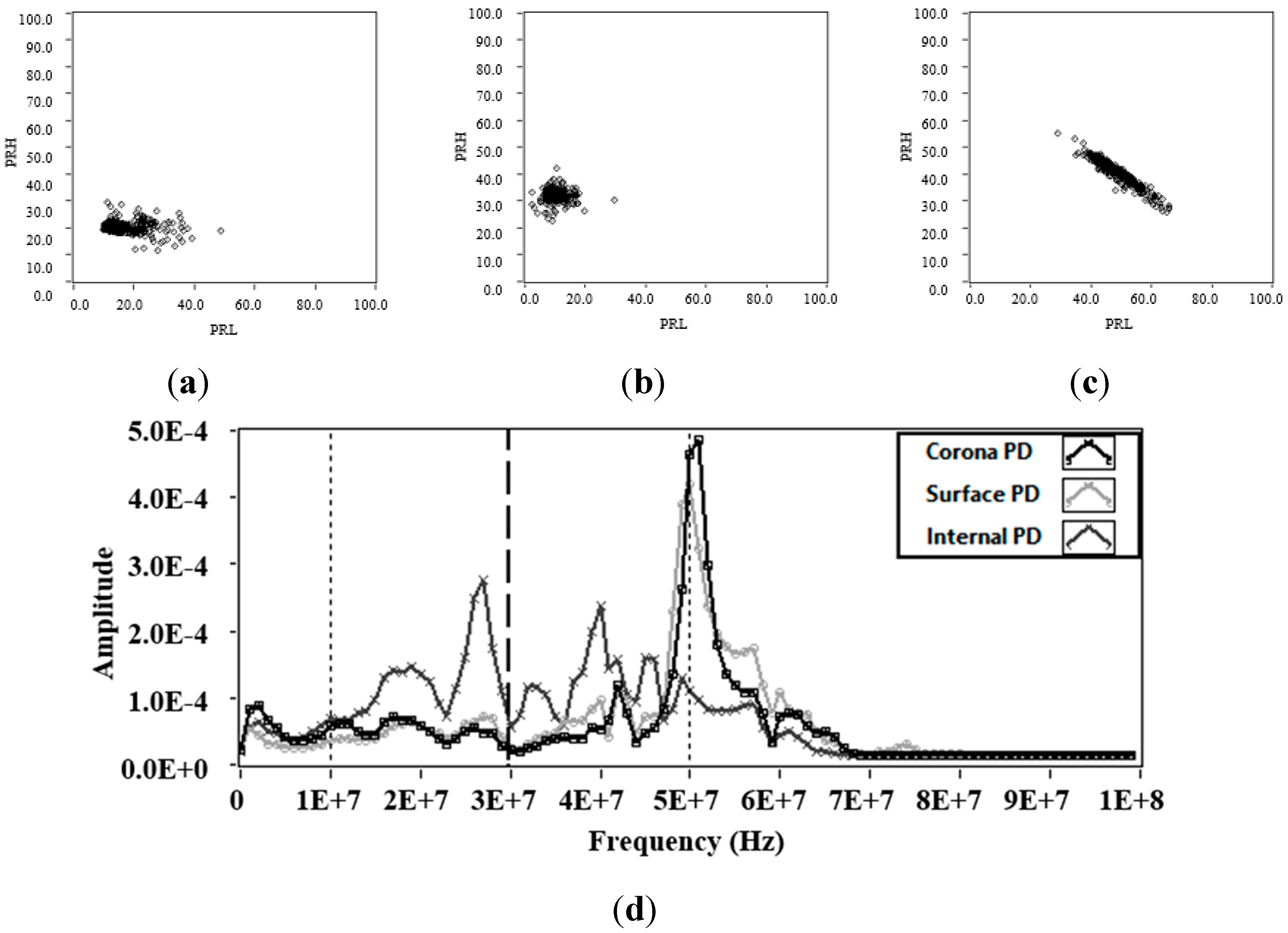
Figure 7a–d represent the PR maps and the average spectral power of the signals measured by applying 5 kV to the point-plane experimental test object, 8.3 kV to the ceramic bushing and 9 kV to the pierced insulating sheets respectively.
Figure 7d shows that the spectral power components detected by the RC in the intervals [10, 30] MHz and [30, 50] MHz are higher for the pulses associated to internal PD (PD in the pierced insulating sheets), this can be confirmed in
Figure 7c, where the position of the cluster with respect to the PRL and PRH axis is higher than that obtained with the clusters of corona and surface PD.
Figure 7d also shows, that for the pulses associated to corona and surface PD, the spectral power detected is very similar in the interval [10, 30] MHz, while in the interval [30, 50] MHz the spectral power is slightly higher for surface PD, which is consistent with the position of the clusters in both classification maps, see
Figure 7a (corona PD) and b (surface PD).
Figure 7.
Partial discharges (a) Power ratio map for PD in point-plane experimental test object; (b) Power ratio map for PD in contaminated ceramic bushing; (c) Power ratio map for PD in pierced insulating sheets; (d) Average spectral power of the PD signals obtained with the three test objects.
Figure 7.
Partial discharges (a) Power ratio map for PD in point-plane experimental test object; (b) Power ratio map for PD in contaminated ceramic bushing; (c) Power ratio map for PD in pierced insulating sheets; (d) Average spectral power of the PD signals obtained with the three test objects.
Regarding the dispersion of the clusters associated to PD (see
Table 3), the results indicate that the internal PD clusters present the higher spectral power dispersion, both in PRL and PRH (5.41 and 4.40, respectively). On the contrary, the dispersion was considerably low for the surface PD clusters, thus together with the fact that the
σPRL/σPRH ratio is close to 1, makes the cluster for this type of source be very homogeneous and with low dispersion. The latter is particularly important because, as will be shown in the next section, a high homogeneity in clusters facilitates the separation task and their subsequent display of the PRPD pattern if there are present several sources acting simultaneously.
In these measurements, it is noted that the dispersion in PRL continues to be higher than that obtained in PRH. Again, the σPRL/σPRH ratio is much greater for the PD obtained for the point-plane experimental test object (3.18).
Table 3.
Results obtained of the standard deviation for each cluster associated with PD.
Table 3.
Results obtained of the standard deviation for each cluster associated with PD.
| Indicator | Corona PD | Surface PD | Internal PD |
|---|
| σPRL | 5.12 | 2.11 | 5.51 |
| σPRH | 1.61 | 1.63 | 4.40 |
| σPRL/σPRH | 3.18 | 1.29 | 1.25 |
4.1.3. PD and Noise Characterization
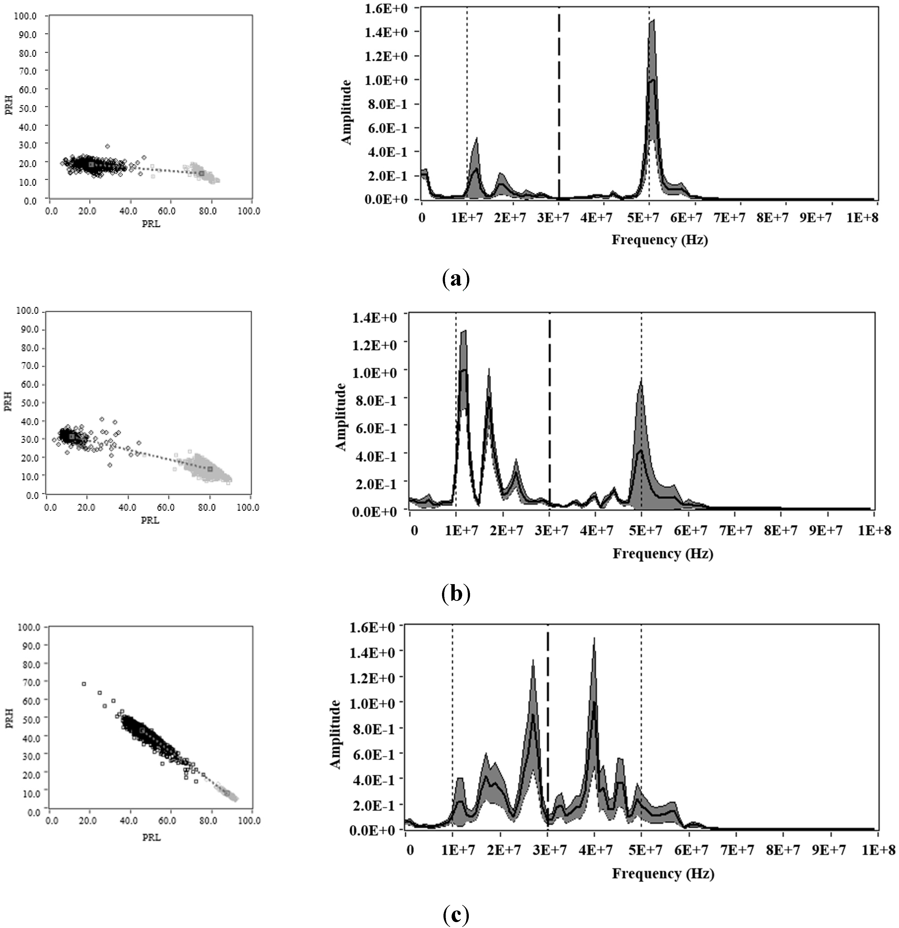
In this section, measurements were performed for each of the test objects with the same voltage level used in the previous section, but with a reduced trigger level (0.4 mV). This was made to enable the acquisition of PD and noise simultaneously.
Figure 8 (left), shows the PR map with the clusters associated to PD (black cluster) and noise (grey cluster).
Figure 8 (right) shows the average power spectrum densities, for each of PD and noise pulses that are represented on the PR map and that are acquired for each test object.
Considering that for this experiment, there are two sources simultaneously acting, the average power spectrum density is presented in order to see if in the selected intervals (f1L = 10 MHz, f2L = f1H = 30 MHz, f2H = 50 MHz, fT = 60 MHz) are included the bands where greater variability of spectral power is presented. If these are included, a clear separation of sources (PD and noise) could be achieved in the PR maps, since for these bands, the captured pulses have less similarity. Otherwise, if the bands with less variability of spectral power are selected, the clusters could be overlapped and the separation of sources could result more difficult. The average of the spectrums is plotted in central thick line; the shaded area corresponds to the area at one standard deviation of the mean that was obtained for the pulses in each measurement.
For each of the experiments, the
K-means algorithm [
23] has been used to identify the clusters and its centroids after applying the SPCT to the pulses measured.
As expected, the clusters associated to PD and noise tend to take similar positions as those observed in
Figure 6 (only noise) and
Figure 7 (only PD). However, the position of the clusters no longer matches with the average spectral power obtained (central thick line), since the spectral content dependent on the spectral power of both types of sources (PD and noise). Therefore, the spectral components will be affected by the two sources acting simultaneously during the acquisition. On the other hand, as was described above, the standard deviation (shaded area) helps to indicate the frequency bands where there is greater statistical variability. With this information, the user can select or modify the frequency bands, in order to improve the separation of sources. Accordingly, for this experiment it is observed that both PRL and PRH include some frequency bands where the standard deviation of the frequency spectra was high. This allows the identification in the three cases, the presence of the two clusters, one associated with PD and other with electrical noise.
Figure 8.
Power ratio maps for PD (black cluster) and noise (grey cluster), left: Average power spectrum densities, right: Obtained for (a) corona PD and noise; (b) surface PD and noise and; (c) internal PD and noise.
Figure 8.
Power ratio maps for PD (black cluster) and noise (grey cluster), left: Average power spectrum densities, right: Obtained for (a) corona PD and noise; (b) surface PD and noise and; (c) internal PD and noise.
Note that, in these intervals, also the frequency bands where the standard deviation is minimal were included; therefore, this separation can be improved if only the bands with the higher standard deviation are selected. When evaluating the dispersion values in PRL and PRH, which are summarized in
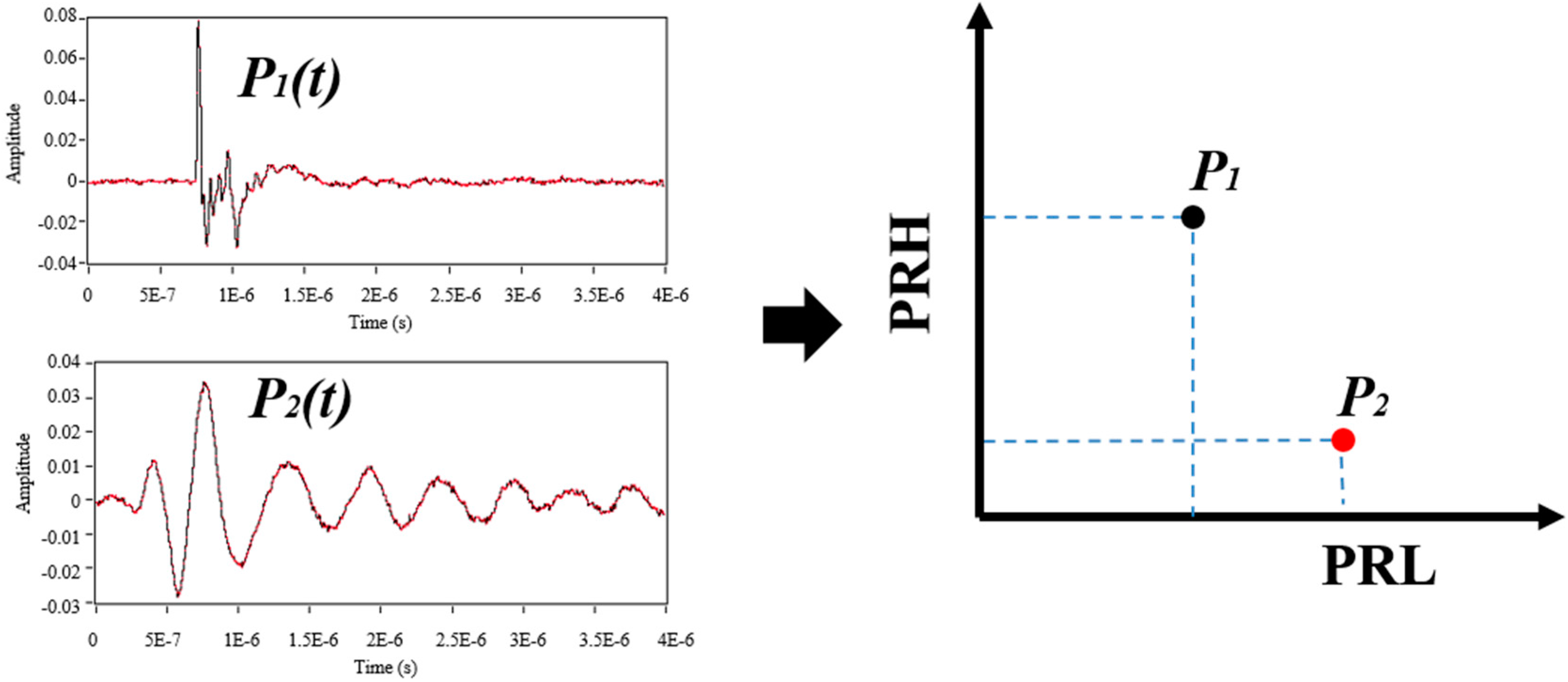
Table 4, it is found that the dispersion in each of the clusters associated with PD was increased. This occurs due to the low trigger level during the acquisition, so the noise pulses can be added to the PD pulses, generating signals with combined spectral power components that cause an increase of the dispersion in the clouds of points. For example, in the case of internal PD and noise in
Figure 8c, that can be considered the most extreme case for having the largest dispersion in PRL and PRH, if it is represented one of the points of the PR map that is located between the two cluster (see
Figure 9), clearly it is observed that the spectral power content of this pulse is formed by components of both sources, see
Figure 6d and
Figure 7d. Due to this, the pulses tend to be located in an intermediate region of the two clusters (critical zone), hindering the separation process and the subsequent identification of the sources.
Table 4.
Results obtained for the standard deviation and its increase in each cluster associated with PD and electrical noise.
Table 4.
Results obtained for the standard deviation and its increase in each cluster associated with PD and electrical noise.
| Indicator | Corona PD and Noise | Surface PD and Noise | Internal PD and Noise |
|---|
| PD | Increase (%) | Noise | PD | Increase (%) | Noise | PD | Increase (%) | Noise |
|---|
| σPRL | 6.69 | 30.66 | 3.10 | 6.02 | 185.30 | 4.28 | 6.71 | 21.77 | 2.42 |
| σPRH | 1.97 | 22.36 | 2.27 | 2.71 | 66.25 | 2.68 | 5.19 | 17.95 | 1.88 |
| σPRL/σPRH | 3.39 | 6.60 | 1.36 | 2.22 | 72.02 | 1.59 | 1.29 | 32.00 | 1.28 |
Figure 9.
Example of a pulse formed by components of PD and noise.
Figure 9.
Example of a pulse formed by components of PD and noise.
However, despite this increase in σPRL and σPRH for each of the clusters associated with PD due to the presence of an additional source of electrical noise, it has been possible to show that the RC allows to characterize adequately in different areas of the map both types of sources by applying the SPCT.
4.2. Experimental Measurements Performed in the Unshielded Laboratory
In order to evaluate the performance of the RC in a less controlled environment, where the noise present has completely different characteristics in time and frequency to those found in the previous experiments, new measurements were carried out in a second high-voltage laboratory. In this second emplacement, there is not any type of shielding that can minimize the presence of external noise sources generated. Additionally, the laboratory is in an area of industrial activity (surrounded by industrial facilities), where the noise level can vary depending on the external activity during the measurement process.
On the other hand, the experimental setup used in this section was prepared to simultaneously generate three different sources: one associated with corona another to internal PD and the last one associated with electrical noise. Thus, the pulse sources were measured with the RC working in a very similar environment to that found in on-site measurements, where most of times it is necessary to detect and separate simultaneous PD and noise sources in order to identify the insulation defects involved.
For this purpose, the tests objects used for internal and corona PD were modified to obtain a stable PD activity for the same voltage level on both test objects (5.2 kV). In this case, the separation from the needle to the ground in the point-plane configuration was 1.5 cm. For the internal defect, the insulation system was composed by eleven insulating sheets of NOMEX where the five central sheets were pierced. Then, an air cylinder with 5 × 0.35 mm in height inside the solid material is obtained. For this experiment, the trigger level was set at 1.3 mV (low), because the maximum noise levels found were close to 2.1 mV, this level of noise is greater than that in the laboratory shielded (1 mV).
Finally, both test objects were electrically connected in parallel and subjected to 5.2 kV, measuring thousands of PD and noise pulses waveforms. The resulting PR map for this experiment, maintaining the same intervals of separation as previously (
f1L = 10 MHz,
f2L =
f1H = 30 MHz,
f2H = 50 MHz,
fT = 60 MHz) is presented in
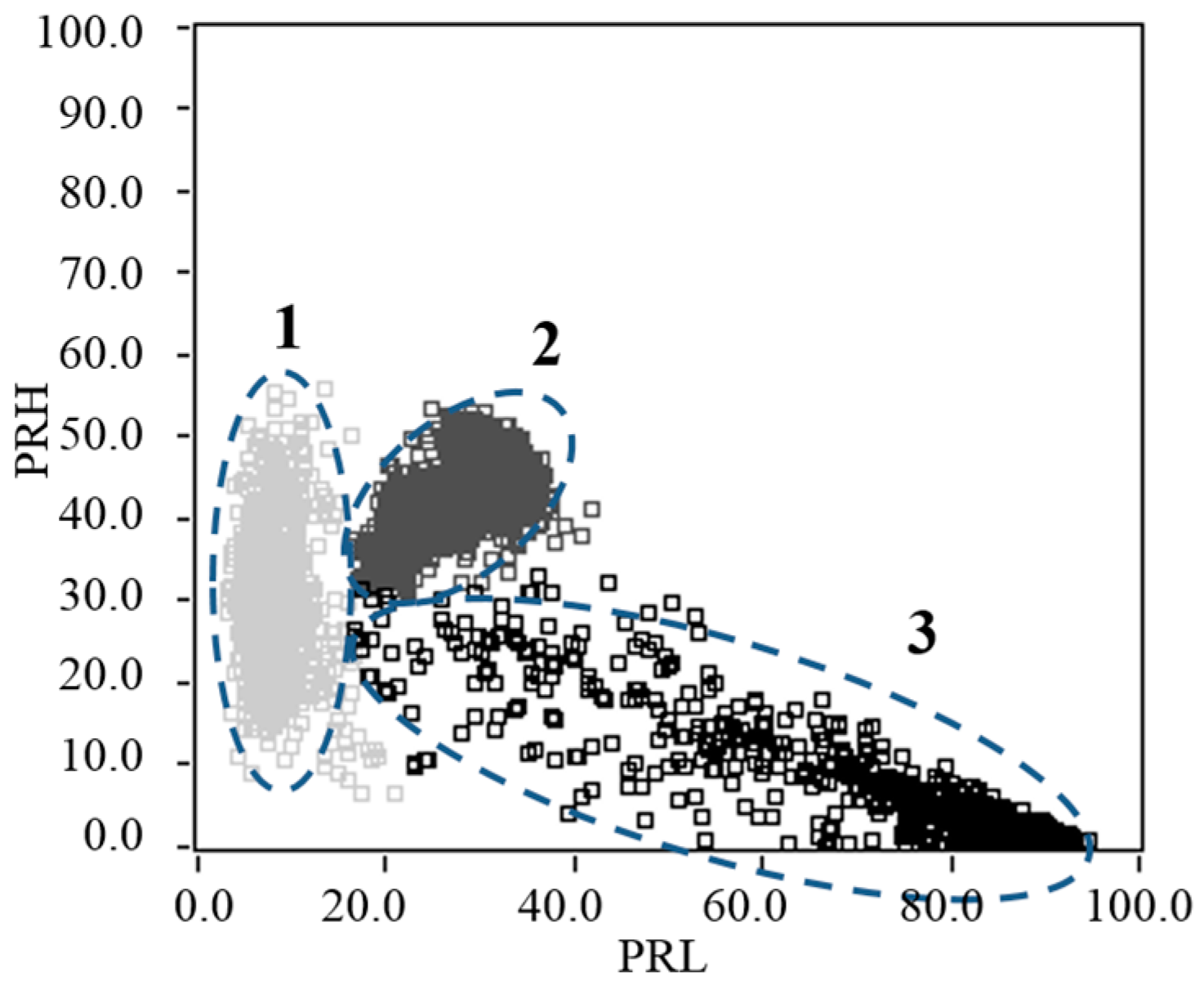
Figure 10. For this case, three different clouds of points can be easily selected (since they are clearly separated) to identify the PD source type through the PRPD patterns.
Figure 10.
PR map obtained for noise (cluster 1), corona PD (cluster 2) and internal PD (cluster 3).
Figure 10.
PR map obtained for noise (cluster 1), corona PD (cluster 2) and internal PD (cluster 3).
The position of the cluster associated with the new source of electrical noise, indicates that the spectral power in the range [10, 30] MHz is lower than that obtained in the previous experiments, in which the source of noise had a high spectral power for the same interval. As for the values of dispersion in PRL and PRH shown in
Table 5, it is seen that the dispersion in PRL is 2.62, lower than previously values previously obtained in
Table 2 for the noise in all the test objects. Contrary to this, the dispersion in PRH is increased almost 292% for the point-plane experimental test object, 247% for the contaminated ceramic bushing and 272% for the pierced insulating sheets; which is consistent with the form taken by this cluster on the PR map and (see
Figure 10). In addition, the
σPRL/σPRH ratio for this new source happened to be well below 1 (0.30).
Table 5.
Results obtained of the standard deviation for each cluster associated with PD and noise.
Table 5.
Results obtained of the standard deviation for each cluster associated with PD and noise.
| Indicator | Noise | Corona PD | Internal PD |
|---|
| σPRL | 2.62 | 4.08 | 11.51 |
| σPRH | 8.75 | 3.68 | 4.45 |
| σPRL/σPRH | 0.30 | 1.10 | 2.58 |
For the cluster associated with corona PD pulses, it was also observed a variation in the shape and the position on the PR map, which differs greatly from previous experiments. The values shown in
Table 5 indicate that the dispersion in PRL and PRH suffered significant changes (
σPRH increases and
σPRL decreases). For this cluster, the new relation
σPRL/σPRH was 1.10. A value close to unit means that the cluster takes a more “symmetric” shape. As mentioned throughout this paper, when it has this kind of geometries or forms in the clusters it facilitates the identification process when the operator have to select the cluster to be represented its respective PRPD pattern, improving the process of identifying the type of source.
Finally, the cluster associated with internal PD also presents great changes, both in position and in shape, according to its PR map characterization. The most notable change, in terms of dispersion, is observed for PRL, which it is increased by almost 108% over the value of PRL obtained in previous experiments (see
Table 3), this is easily seen in the PR map in
Figure 10, where the cluster occupies a large map space due to its lack of homogeneity in this axis. In this case, the relationship
σPRL/σPRH (2.58) indicates an increase of almost 106% compared to the values previously obtained when the size of the vacuole was lower.
These results confirm those described in [
10,
15], where is disclosed that any change of the equivalent capacity in the measuring circuit can vary the shapes and positions of the clusters on the classification map. These variations can be due to the process of manufacturing the test objects or by the fact of perform measurements in an environment where noise levels are different in nature and magnitude than those found in more controlled environments. Therefore, it is very important to properly select the separation intervals depending on the scenario to obtain a clear characterization of all sources present during the measurements.
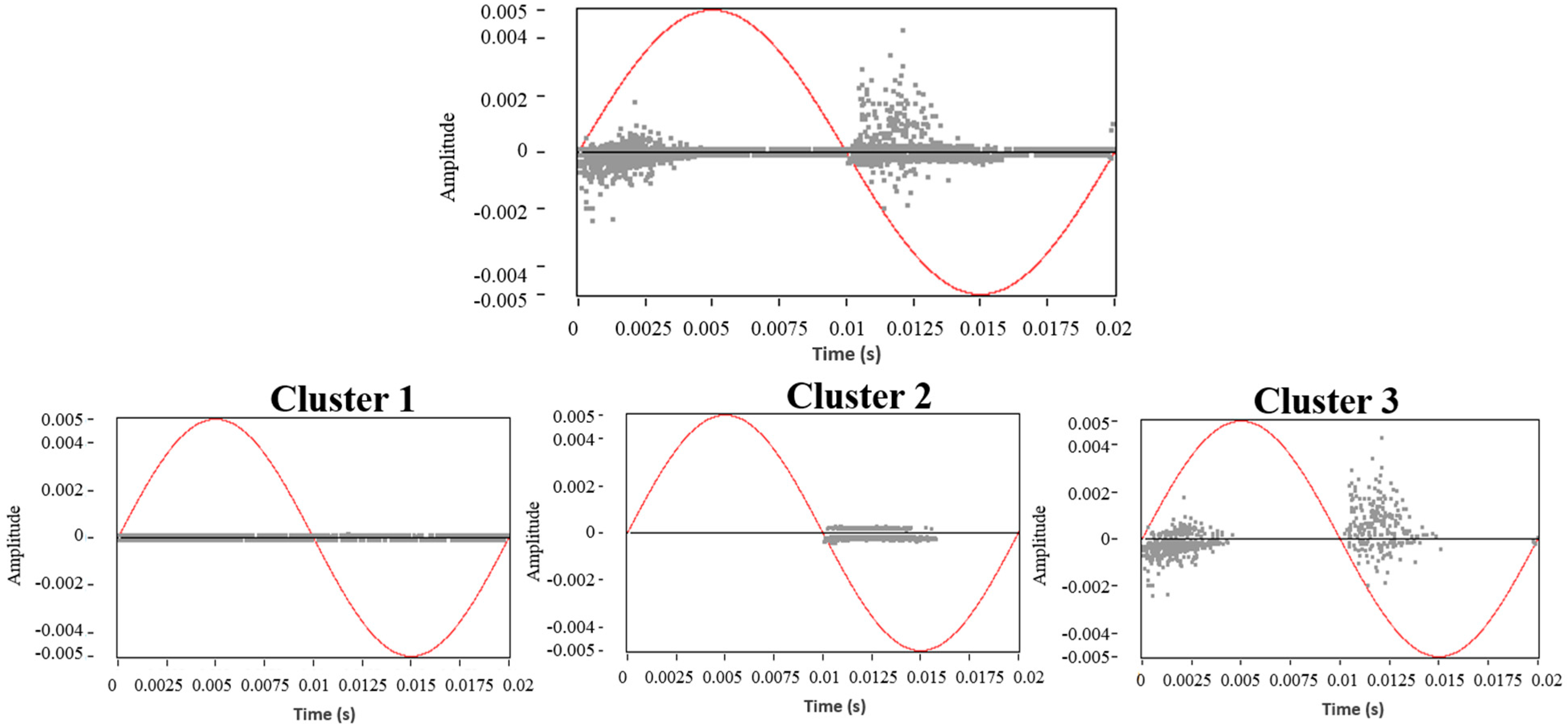
The complete PRPD pattern, for the three PD sources acting simultaneously, is shown in
Figure 11 (Up), where it is clear that PRPD interpretation seems to be quite complex even for an expert in the field. However, if the PRPD pattern for each cluster is represented individually, it can be clearly identify each of the sources present during the acquisition. As it can be seen in
Figure 11 (Down), the PRPD associated to the cluster 1 represents the captured electrical noise during the acquisition (uncorrelated pulses in phase). The PRPD of the cluster 2 corresponds to the typical PRPD for corona discharges, where highly stable PD magnitudes are observed for the negative maxima of the applied voltage. Finally, when selecting the cluster 3 from the PR map provides a “clean” PRPD representation typical from internal PD, where the high-magnitude discharges occur in the phase positions where the voltage slope is maximum.
Figure 11.
PRPD pattern for noise and PD simultaneously, Up: PRPD patterns for Down: cluster 1 (noise), cluster 2 (corona PD), and cluster 3 (internal PD).
Figure 11.
PRPD pattern for noise and PD simultaneously, Up: PRPD patterns for Down: cluster 1 (noise), cluster 2 (corona PD), and cluster 3 (internal PD).
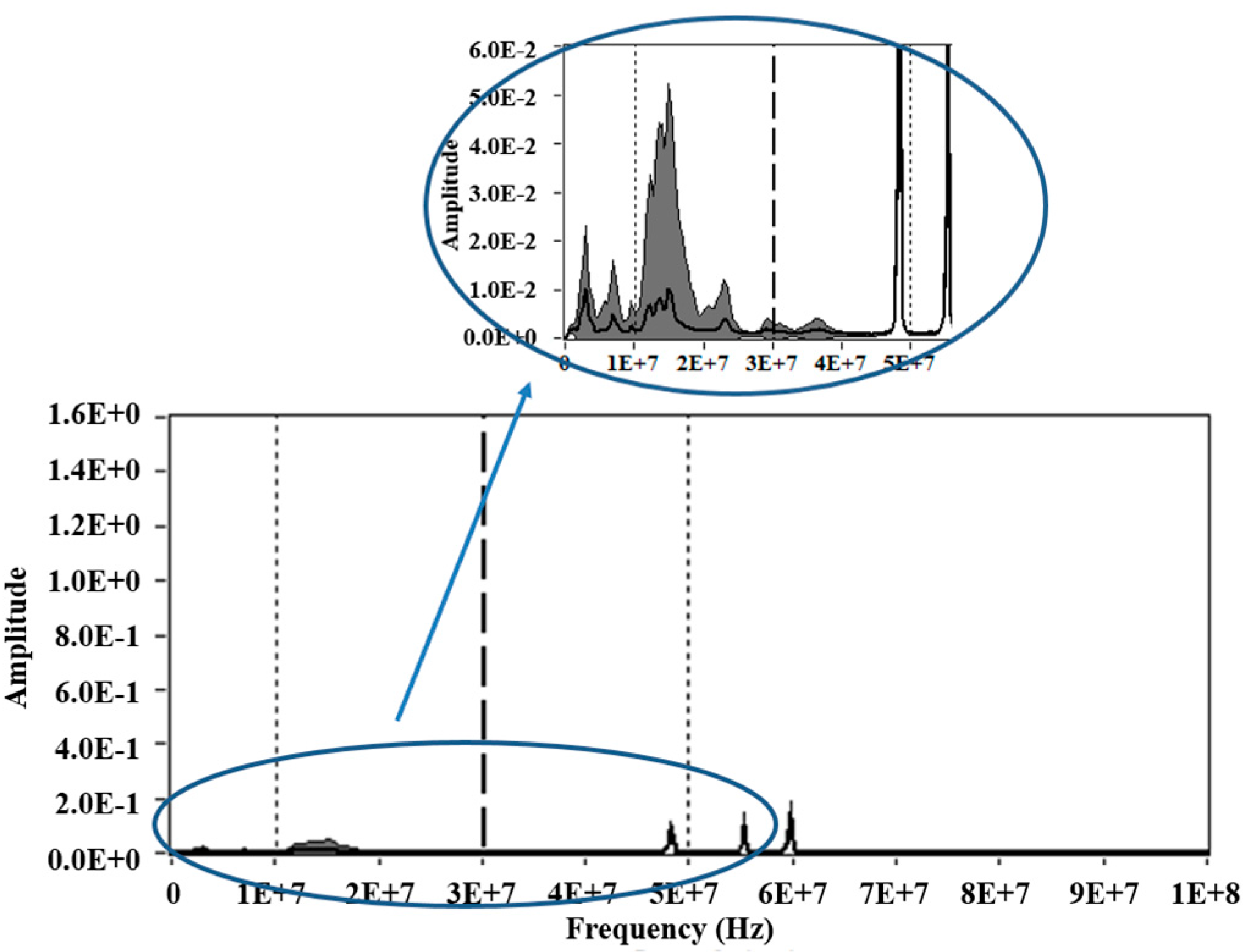
Accordingly, when assessing the average power spectrum density of the pulses obtained in this experiment, it is observed that the selected intervals for PRL [10, 30] MHz and PRH [30, 50] MHz match bands where greater variability of spectral power occurs, that it is shown in the enlarged view in
Figure 12. This justifies the separation obtained for each source on the PR map shown (see
Figure 10).
Figure 12.
Average power spectrum density for PD and noise simultaneously measured.
Figure 12.
Average power spectrum density for PD and noise simultaneously measured.
On the contrary, if the PRL and PRH had other bands, where the variability of spectral power was lower, the separation of the sources would be impossible. This can be demonstrated if the intervals [20, 40] MHz for PRL and [40, 60] MHz for PRH are used, for example. As shown in the PR map in
Figure 13 (Left), using these new intervals of separation (including bands where the variability of spectral power is low), only two different clusters can be identify, which they are also very close each other. Therefore, two types of sources are superimposed in a single cluster, this can be checked representing the PRPD patterns for each cluster, see
Figure 13 (Right). In the PR map of the
Figure 13, the cluster 2 corresponds to the electrical noise, while the cluster 1 corresponds with the two types of the two remaining sources (corona and Internal PD), which are clearly overlapping.
Figure 13.
PR map for simultaneous PD (corona and internal) and noise activity. Frequency intervals for the power ratios calculations: f1L = 20 MHz, f2L = 40 MHz, f1H = 40 MHz, f2H = 60 MHz.
Figure 13.
PR map for simultaneous PD (corona and internal) and noise activity. Frequency intervals for the power ratios calculations: f1L = 20 MHz, f2L = 40 MHz, f1H = 40 MHz, f2H = 60 MHz.
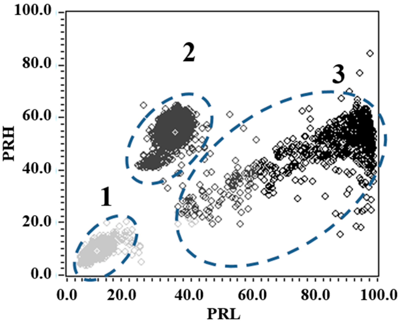
Likewise, if other intervals, in which the frequency bands present greater variability of spectral power are selected, the sources separation will become more effective. For example, if
f1L = 2 MHz,
f2L =25 MHZ,
f1H = 15 MHz,
f2H = 38 MHz (
fT = 60 MHz), intervals are used, a better separation between clusters is achieved (see
Figure 14), compared with the separation obtained with the intervals used previously, see
Figure 10 and
Figure 13.
Figure 14.
PR map for simultaneous PD and noise activity. Frequency intervals for the power ratios calculations: f1L = 2 MHz, f2L = 25 MHz, f1H = 15 MHz, f2H = 38 MHz.
Figure 14.
PR map for simultaneous PD and noise activity. Frequency intervals for the power ratios calculations: f1L = 2 MHz, f2L = 25 MHz, f1H = 15 MHz, f2H = 38 MHz.
In this new separation map, the cluster 1 is associated with electrical noise pulses, cluster 2 with corona PD and cluster 3 with internal PD. Analysing the values of dispersion for PRL and PRH that are presented in
Table 6, except
σPRL for corona PD cluster and
σPRH for internal PD, a clear decrease in the dispersion for each of the clusters using these new separation intervals it is shown. Additionally, a marked improvement in the
σPRL/σPRH relation to the case of clusters associated with internal PD and electrical noise was achieved, since values close to 1 were obtained compared to the values shown in
Table 5. For the cluster associated with corona PD, this relationship is increased, but not very significantly (1.35) compared to the previous value obtained in
Table 5 (1.10).
Table 6.
Results obtained of the standard deviation for each cluster associated with PD and noise, using f1L = 2 MHz, f2L =25 MHZ, f1H = 15 MHz, f2H = 38 MHz, fT = 60 MHz intervals.
Table 6.
Results obtained of the standard deviation for each cluster associated with PD and noise, using f1L = 2 MHz, f2L =25 MHZ, f1H = 15 MHz, f2H = 38 MHz, fT = 60 MHz intervals.
| Indicator | Noise | Corona PD | Internal PD |
|---|
| σPRL | 2.35 | 4.66 | 6.55 |
| σPRH | 2.56 | 3.45 | 9.72 |
| σPRL/σPRH | 0.91 | 1.35 | 0.67 |


