
Pedestrian Navigation Using Foot-Mounted Inertial Sensor and LIDAR


Abstract
:1. Introduction
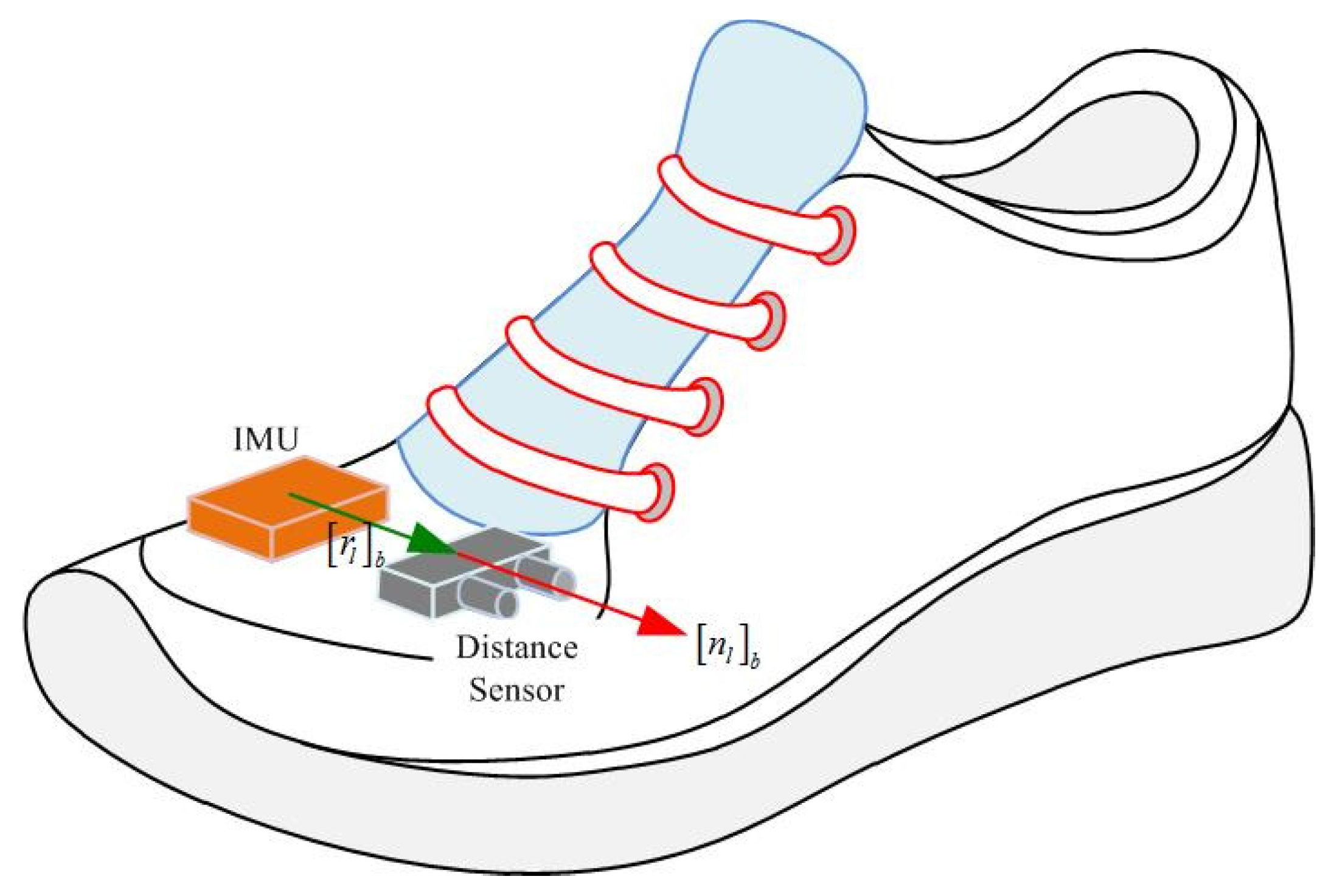
2. Overview System


3. Distance Sensor Calibration

4. Kalman Filter Combining an INA and Compensation Using LIDAR
4.1. Basic INA
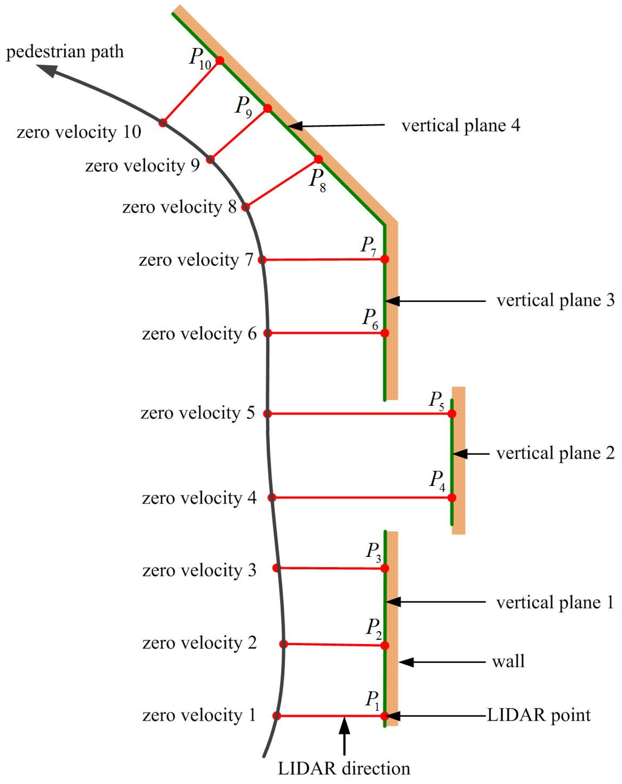
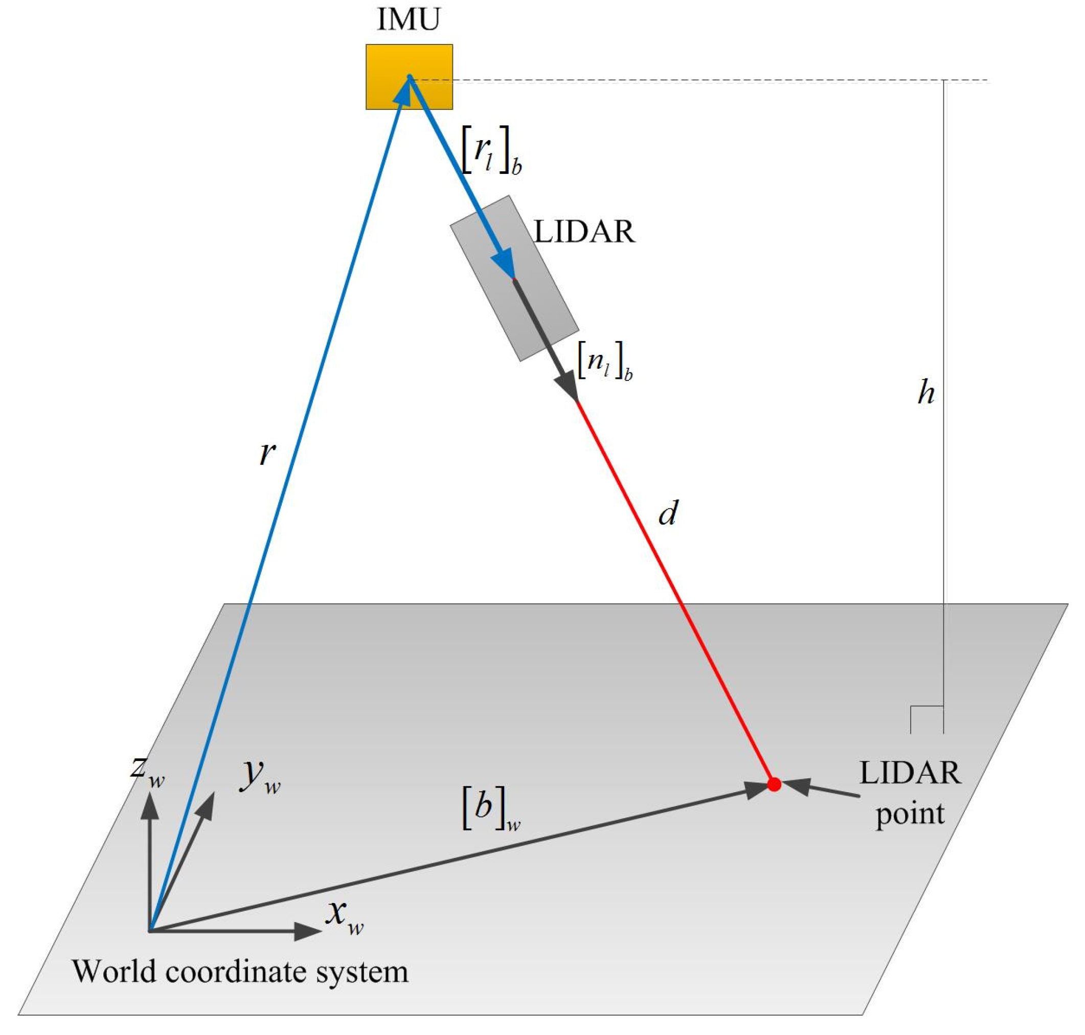
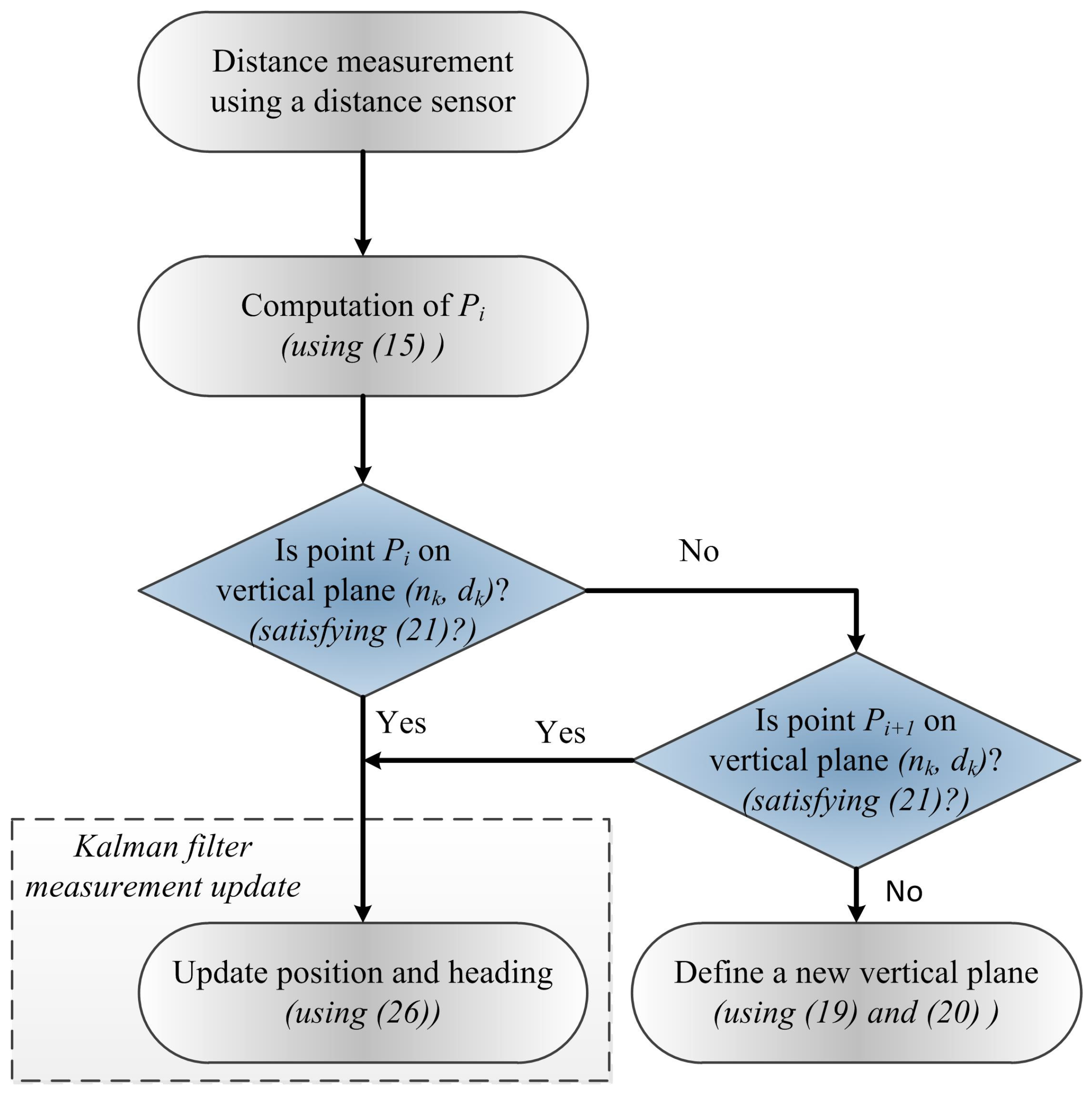
4.2. Proposed Position and Heading Updating Algorithm Using the Distance Sensor


5. Experiments and Results


| Experiment Number | Position Error (Pure INA) | Position Error (Proposed Method) |
|---|---|---|
| 1 | 4.38 | 1.74 |
| 2 | 9.48 | 1.55 |
| 3 | 10.48 | 1.54 |
| 4 | 11.61 | 1.40 |
| 5 | 8.50 | 1.43 |
| RMS | 9.23 | 1.54 |
| Experiment Number | Walking Speed (km/h) | Stride Length (m) | Stride Speed (stride/s) | Position Error (Pure INA) (m) | Position Error (Proposed Method) (m) |
|---|---|---|---|---|---|
| 1 | 4.14 | 1.25 | 0.92 | 2.04 | 0.45 |
| 2 | 4.15 | 1.25 | 0.92 | 1.32 | 0.34 |
| 3 | 4.57 | 1.25 | 1.02 | 2.57 | 0.52 |
| 4 | 4.59 | 1.30 | 0.98 | 3.21 | 0.54 |
| 5 | 4.72 | 1.30 | 1.01 | 3.11 | 0.37 |
| 6 | 5.19 | 1.50 | 0.96 | 2.25 | 0.43 |
| 7 | 5.43 | 1.50 | 1.01 | 1.67 | 0.35 |
| 8 | 5.44 | 1.50 | 1.01 | 1.70 | 0.44 |
| 9 | 5.46 | 1.50 | 1.01 | 2.53 | 0.52 |
| 10 | 5.53 | 1.50 | 1.02 | 1.22 | 0.36 |
| 11 | 5.54 | 1.50 | 1.03 | 1.26 | 0.42 |
| 12 | 5.57 | 1.50 | 1.03 | 2.33 | 0.37 |
| 13 | 6.06 | 1.50 | 1.12 | 2.58 | 0.39 |
| 14 | 6.07 | 1.50 | 1.12 | 0.84 | 0.31 |
| 15 | 6.10 | 1.50 | 1.13 | 1.80 | 0.51 |
| Mean | 2.03 | 0.42 | |||


| Experiment Number | Position Error (Pure INA) | Position Error (Proposed Method) |
|---|---|---|
| 1 | 3.01 | 0.20 |
| 2 | 5.20 | 0.64 |
| 3 | 1.94 | 0.64 |
| 4 | 2.67 | 0.91 |
| 5 | 5.32 | 0.13 |
| RMS | 3.88 | 0.58 |
6. Discussion


| Stride Speed (Stride/s) | Walking Speed (km/h) | Stride Length (m) | Number Zero Velocity Interval (True) | Missing Zero Velocity Detection |
|---|---|---|---|---|
| 0.92 | 4.14 | 1.25 | 25 | 0 |
| 0.96 | 5.19 | 1.50 | 21 | 0 |
| 0.98 | 4.59 | 1.30 | 24 | 0 |
| 1.01 | 4.72 | 1.30 | 24 | 0 |
| 1.01 | 5.46 | 1.50 | 21 | 0 |
| 1.01 | 5.44 | 1.50 | 21 | 0 |
| 1.01 | 5.43 | 1.50 | 21 | 0 |
| 1.02 | 4.57 | 1.25 | 25 | 0 |
| 1.02 | 5.53 | 1.50 | 21 | 0 |
| 1.03 | 5.57 | 1.50 | 21 | 0 |
| 1.03 | 5.54 | 1.50 | 21 | 0 |
| 1.12 | 6.06 | 1.50 | 21 | 0 |
| 1.12 | 6.07 | 1.50 | 21 | 0 |
| 1.13 | 6.10 | 1.50 | 21 | 1 |
| 1.16 | 5.96 | 1.43 | 22 | 4 |
| 1.17 | 6.04 | 1.43 | 22 | 8 |
| 1.26 | 6.78 | 1.50 | 21 | 17 |
| 1.28 | 6.94 | 1.50 | 21 | 18 |
| 1.32 | 6.81 | 1.43 | 22 | 19 |
| 1.35 | 6.95 | 1.43 | 22 | 18 |
7. Conclusions
Acknowledgments
Author Contributions
Conflicts of Interest
References
- Chen, L.; Hu, H. IMU/GPS based pedestrian localization. In Proceedings of the 2012 4th Computer Science and Electronic Engineering Conference, Colchester, UK, 12–13 September 2012; pp. 23–28.
- Langer, M.; Kiesel, S.; Ascher, C.; Trommer, G. Deeply Coupled GPS/INS integration in pedestrian navigation systems in weak signal conditions. In Proceedings of the 2012 International Conference on Indoor Positioning and Indoor Navigation, Sydney, Australia, 13–15 November 2012; pp. 1–7.
- Chen, G.; Meng, X.; Wang, Y.; Zhang, Y.; Tian, P.; Yang, H. Integrated WiFi/PDR/Smartphone Using an Unscented Kalman Filter Algorithm for 3D Indoor Localization. Sensors 2015, 15, 24595–24614. [Google Scholar] [CrossRef] [PubMed]
- Deng, Z.A.; Wang, G.; Hu, Y.; Wu, D. Heading Estimation for Indoor Pedestrian Navigation Using a Smartphone in the Pocket. Sensors 2015, 15, 21518–21536. [Google Scholar] [CrossRef] [PubMed]
- Jimenez, A.; Seco, F.; Prieto, J.; Guevara, J. Indoor pedestrian navigation using an INS/EKF framework for yaw drift reduction and a foot-mounted IMU. In Proceedings of the 2010 7th Workshop on Positioning Navigation and Communication, Dresden, Germany, 11–12 March 2010; pp. 135–143.
- Renaudin, V.; Combettes, C. Magnetic, Acceleration Fields and Gyroscope Quaternion (MAGYQ)-Based Attitude Estimation with Smartphone Sensors for Indoor Pedestrian Navigation. Sensors 2014, 14, 22864–22890. [Google Scholar] [CrossRef] [PubMed]
- Placer, M.; Kovacic, S. Enhancing Indoor Inertial Pedestrian Navigation Using a Shoe-Worn Marker. Sensors 2013, 13, 9836–9859. [Google Scholar] [CrossRef] [PubMed]
- Jin, Y.; Motani, M.; Soh, W.S.; Zhang, J. SparseTrack: Enhancing Indoor Pedestrian Tracking with Sparse Infrastructure Support. In Proceedings of the IEEE INFOCOM, San Diego, CA, USA, 14–19 March 2010; pp. 1–9.
- He, Z.; Renaudin, V.; Petovello, M.G.; Lachapelle, G. Use of High Sensitivity GNSS Receiver Doppler Measurements for Indoor Pedestrian Dead Reckoning. Sensors 2013, 13, 4303–4326. [Google Scholar] [CrossRef] [PubMed]
- Broggi, A.; Cerri, P.; Ghidoni, S.; Grisleri, P.; Jung, H.G. A New Approach to Urban Pedestrian Detection for Automatic Braking. IEEE Trans. Intell. Transp. Syst. 2009, 10, 594–605. [Google Scholar] [CrossRef]
- Baranski, P.; Strumillo, P. Enhancing Positioning Accuracy in Urban Terrain by Fusing Data from a GPS Receiver, Inertial Sensors, Stereo-Camera and Digital Maps for Pedestrian Navigation. Sensors 2012, 12, 6764–6801. [Google Scholar] [CrossRef] [PubMed]
- Dickens, J.; van Wyk, M.; Green, J. Pedestrian detection for underground mine vehicles using thermal images. In Proceedings of the AFRICON, Livingstone, South Africa, 13–15 September 2011; pp. 1–6.
- Yuan, Y.; Chen, C.; Guan, X.; Yang, Q. An Energy-Efficient Underground Localization System Based on Heterogeneous Wireless Networks. Sensors 2015, 15, 12358–12376. [Google Scholar] [CrossRef] [PubMed]
- Liu, Z.; Li, C.; Wu, D.; Dai, W.; Geng, S.; Ding, Q. A Wireless Sensor Network Based Personnel Positioning Scheme in Coal Mines with Blind Areas. Sensors 2010, 10, 9891–9918. [Google Scholar] [CrossRef] [PubMed]
- Hightower, J.; Borriello, G. Location Systems for Ubiquitous Computing. Computer 2001, 34, 57–66. [Google Scholar] [CrossRef]
- Ruiz, A.; Granja, F.; Prieto Honorato, J.; Rosas, J. Accurate Pedestrian Indoor Navigation by Tightly Coupling Foot-Mounted IMU and RFID Measurements. IEEE Trans. Instrum. Meas. 2012, 61, 178–189. [Google Scholar] [CrossRef]
- Amendolare, V.; Cyganski, D.; Duckworth, R.; Makarov, S.; Coyne, J.; Daempfling, H.; Woodacre, B. WPI precision personnel locator system: Inertial navigation supplementation. In Proceedings of the IEEE/ION Position, Location and Navigation Symposium, Monterey, CA, USA, 5–8 May 2008; pp. 350–357.
- Fischer, C.; Muthukrishnan, K.; Hazas, M.; Gellersen, H. Ultrasound-aided Pedestrian Dead Reckoning for Indoor Navigation. In Proceedings of the 1st ACM International Workshop on Mobile Entity Localization and Tracking in GPS-less Environments, San Francisco, CA, USA, 19 September 2008; pp. 31–36.
- Zhou, C.; Downey, J.; Stancil, D.; Mukherjee, T. A Low-Power Shoe-Embedded Radar for Aiding Pedestrian Inertial Navigation. IEEE Trans. Microw. Theory Tech. 2010, 58, 2521–2528. [Google Scholar] [CrossRef]
- Duong, P.D.; Suh, Y.S. Foot Pose Estimation Using an Inertial Sensor Unit and Two Distance Sensors. Sensors 2015, 15, 15888–15902. [Google Scholar] [CrossRef] [PubMed]
- Xu, Z.; Wei, J.; Zhang, B.; Yang, W. A Robust Method to Detect Zero Velocity for Improved 3D Personal Navigation Using Inertial Sensors. Sensors 2015, 15, 7708–7727. [Google Scholar] [CrossRef] [PubMed]
- STMicroelectronics. LIDAR (Light Detection and Ranging Module) Datasheet. Available online: https://cdn.sparkfun.com/datasheets/Sensors/Proximity/lidarlite2DS.pdf (accessed on 19 January 2016).
- Nam, C.N.K.; Kang, H.J.; Suh, Y.S. Golf Swing Motion Tracking Using Inertial Sensors and a Stereo Camera. IEEE Trans. Instrum. Meas. 2014, 63, 943–952. [Google Scholar] [CrossRef]
- Titterton, D.H.; Weston, J.L. Strapdown Inertial Navigation Technology; Peter Peregrinus Ltd.: London, UK, 1997. [Google Scholar]
- Kuipers, J.B. Quaternions and Rotation Sequences: A Primer with Applications to Orbits, Aerospace, and Virtual Reality; Princeton University Press: Princeton, NJ, USA, 1999. [Google Scholar]
- Savage, P.G. Strapdown Inertial Navigation Integration Algorithm Design Part 1: Attitude Algorithms. J. Guid. Control Dyn. 1998, 21, 19–28. [Google Scholar] [CrossRef]
- Markley, F.L. Multiplicative vs. Additive Filtering for Spacecraft Attitude Determination. In Proceedings of the 6th Cranfield Conference on Dynamics and Control of Systems and Structures in Space, Riomaggiore, Italy, 18–22 July 2004; pp. 467–474.
- Suh, Y.S.; Park, S. Pedestrian Inertial Navigation with Gait Phase Detection Assisted Zero Velocity Updating. In Proceedings of the 4th International Conference on Autonomous Robots and Agents, Wellington, New Zealand, 10–12 February 2009; pp. 336–341.
- Hawkinson, W.; Samanant, P.; McCroskey, R.; Ingvalson, R.; Kulkarni, A.; Haas, L.; English, B. GLANSER: Geospatial Location, Accountability, and Navigation System For Emergency Responders. In Proceedings of the Position Location and Navigation Symposium, Myrtle Beach, SC, 24–26 April 2012; pp. 98–105.
- Park, S.K.; Suh, Y.S. A Zero Velocity Detection Algorithm Using Inertial Sensors for Pedestrian Navigation Systems. Sensors 2010, 10, 9163–9178. [Google Scholar] [CrossRef] [PubMed]
- Skog, I.; Nilsson, J.O.; Handel, P. Evaluation of zero-velocity detectors for foot-mounted inertial navigation systems. In Proceedings of the International Conference on Indoor Positioning and Indoor Navigation, Zurich, Switzerland, 15–17 September 2010; pp. 1–6.
- Markley, F.L.; Crassidis, J.L. Fundamentals of Spacecraft Attitude Determination and Control; Springer: New York, NY, USA, 2014. [Google Scholar]
© 2016 by the authors; licensee MDPI, Basel, Switzerland. This article is an open access article distributed under the terms and conditions of the Creative Commons by Attribution (CC-BY) license (http://creativecommons.org/licenses/by/4.0/).
Share and Cite
Pham, D.D.; Suh, Y.S. Pedestrian Navigation Using Foot-Mounted Inertial Sensor and LIDAR. Sensors 2016, 16, 120. https://0-doi-org.brum.beds.ac.uk/10.3390/s16010120
Pham DD, Suh YS. Pedestrian Navigation Using Foot-Mounted Inertial Sensor and LIDAR. Sensors. 2016; 16(1):120. https://0-doi-org.brum.beds.ac.uk/10.3390/s16010120
Chicago/Turabian StylePham, Duy Duong, and Young Soo Suh. 2016. "Pedestrian Navigation Using Foot-Mounted Inertial Sensor and LIDAR" Sensors 16, no. 1: 120. https://0-doi-org.brum.beds.ac.uk/10.3390/s16010120