
Machine Learning and Computer Vision System for Phenotype Data Acquisition and Analysis in Plants


Abstract
:1. Introduction
2. Materials and Methods
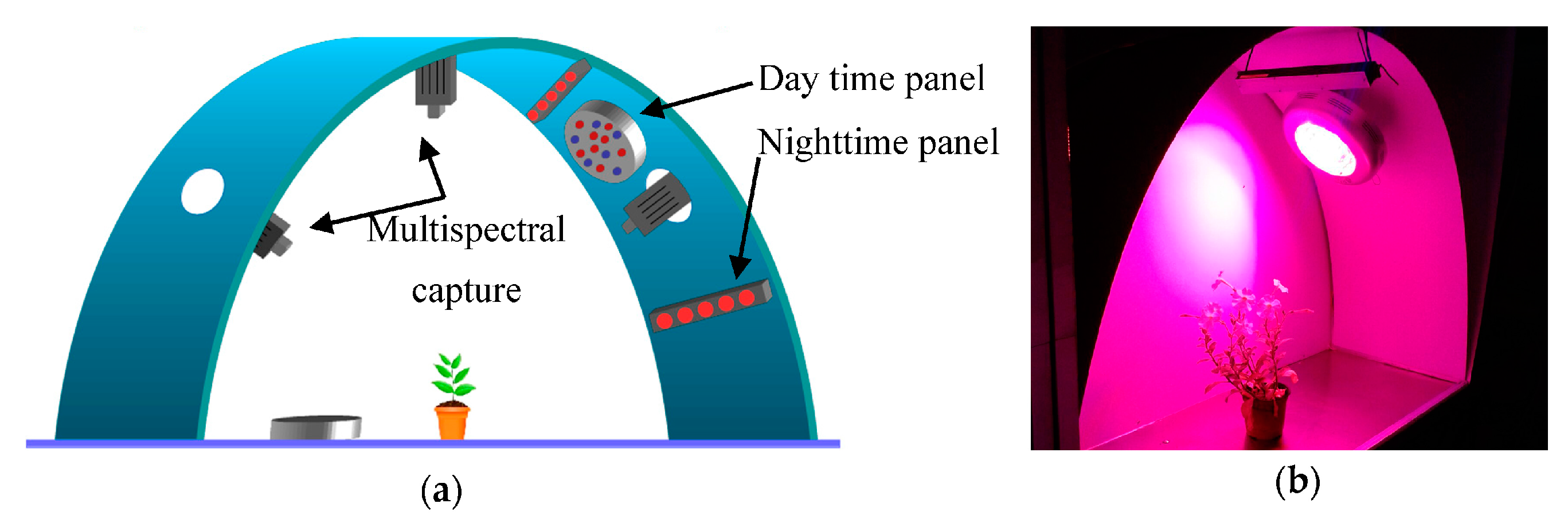
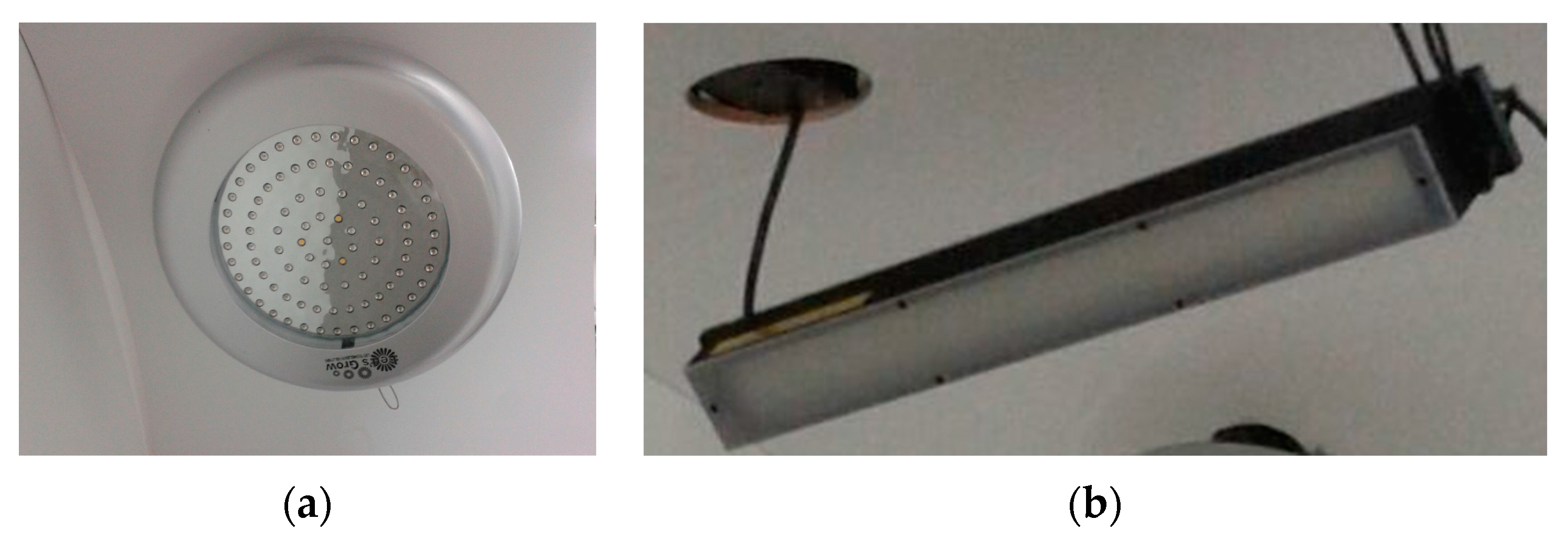
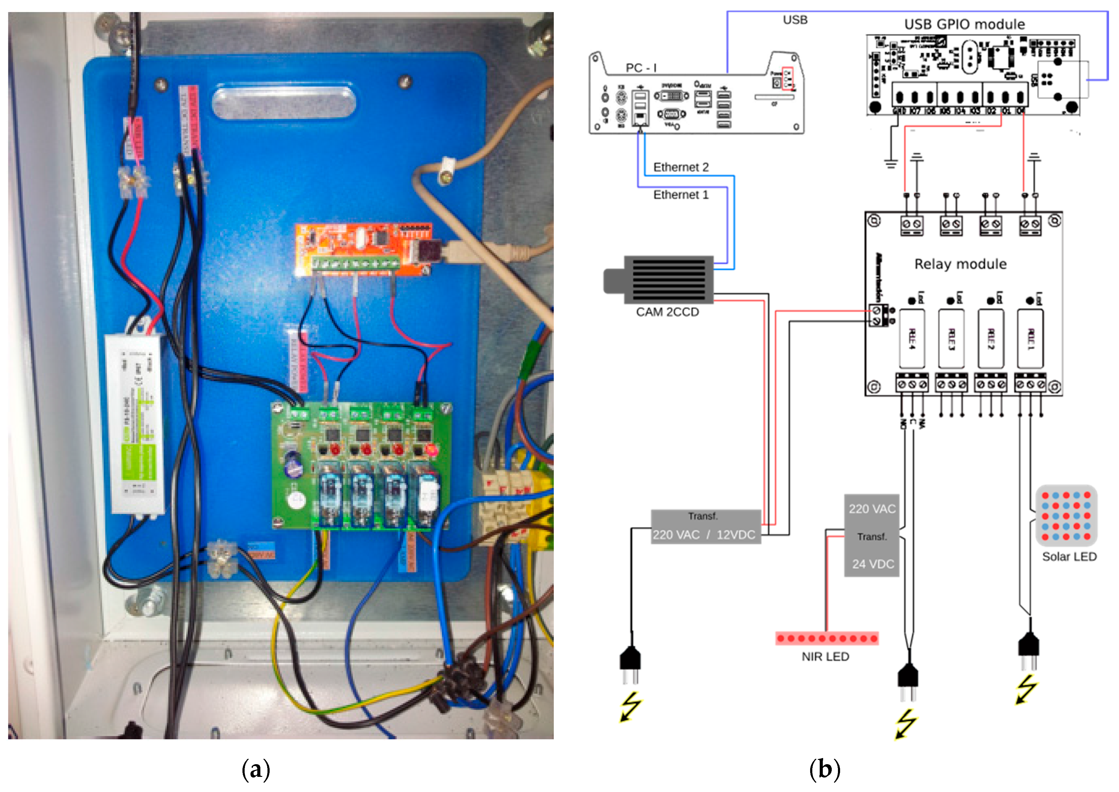
2.1. Ilumination Subsystem
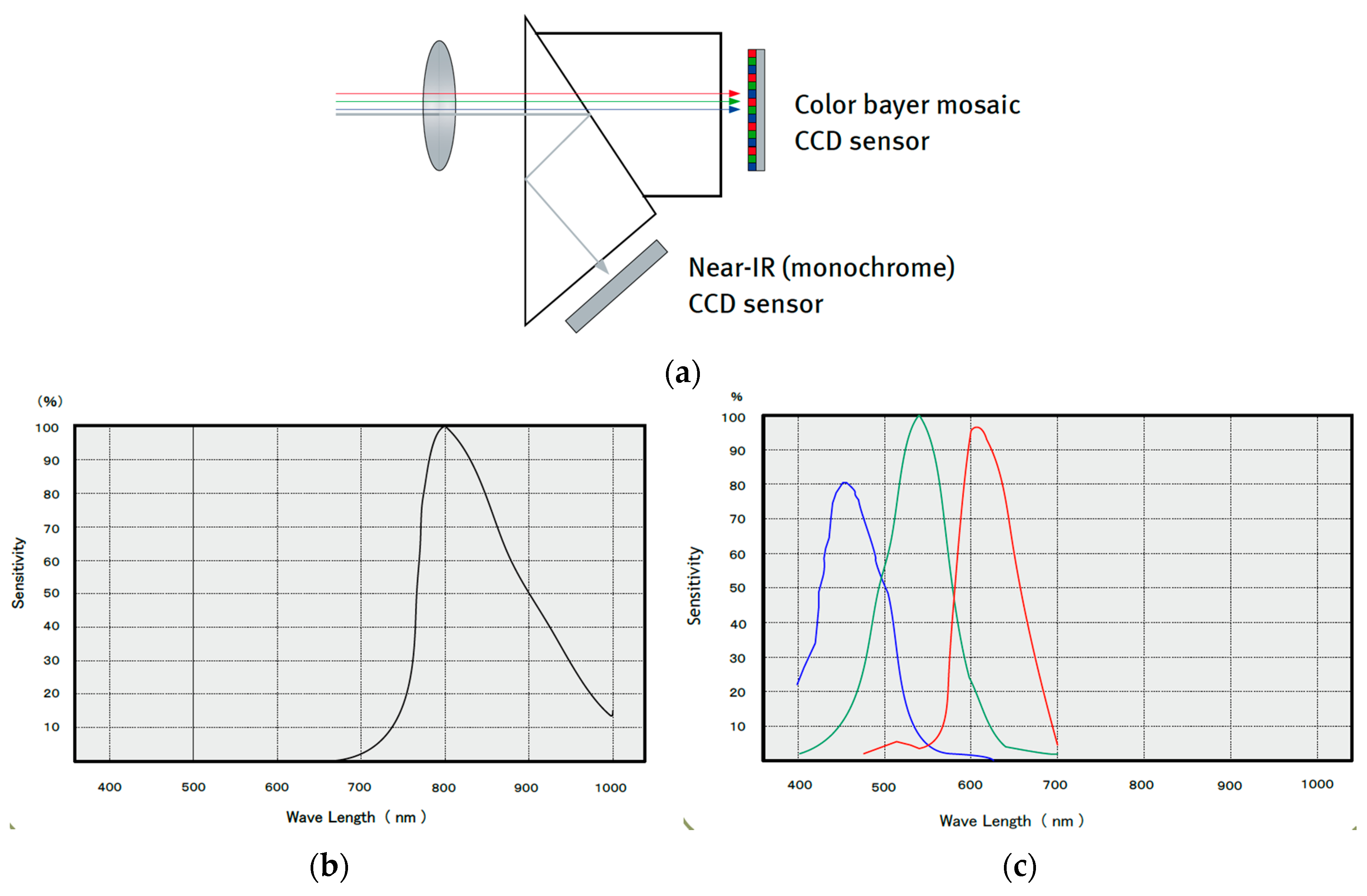
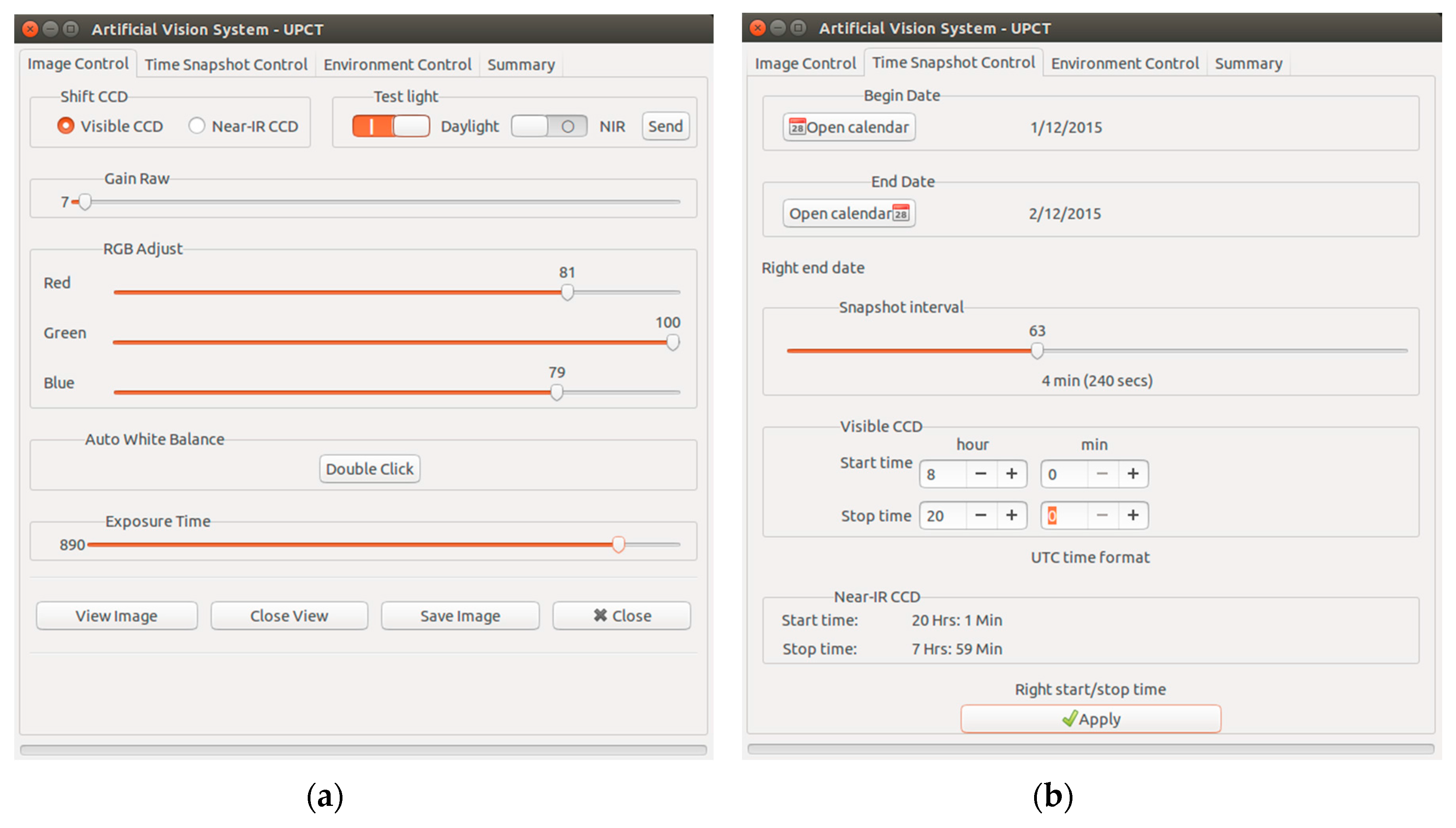
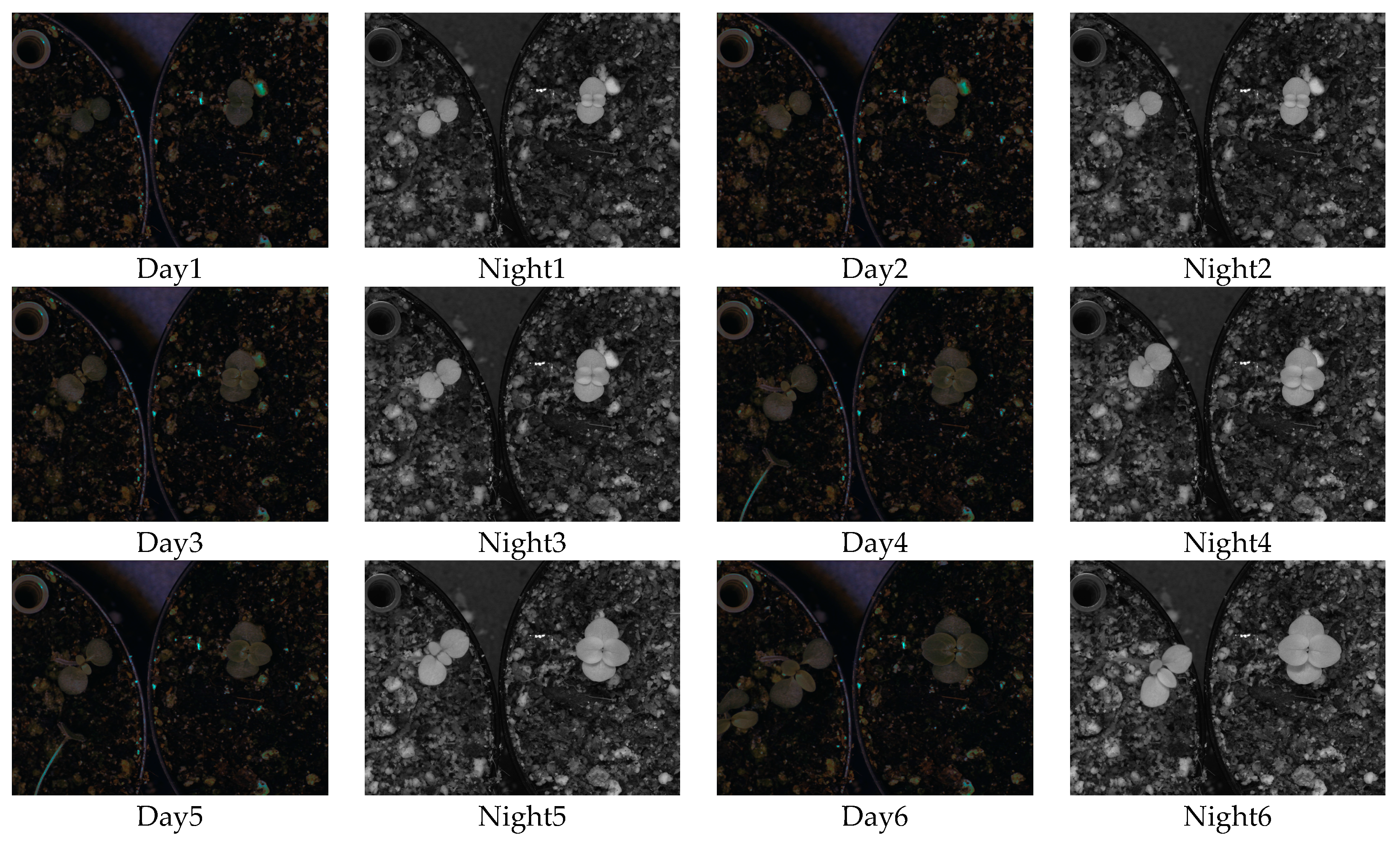
2.2. Capture Subsystem
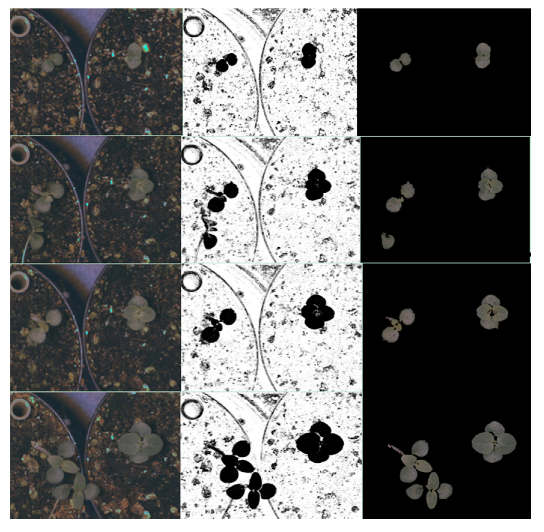
2.3. Image Processing Module
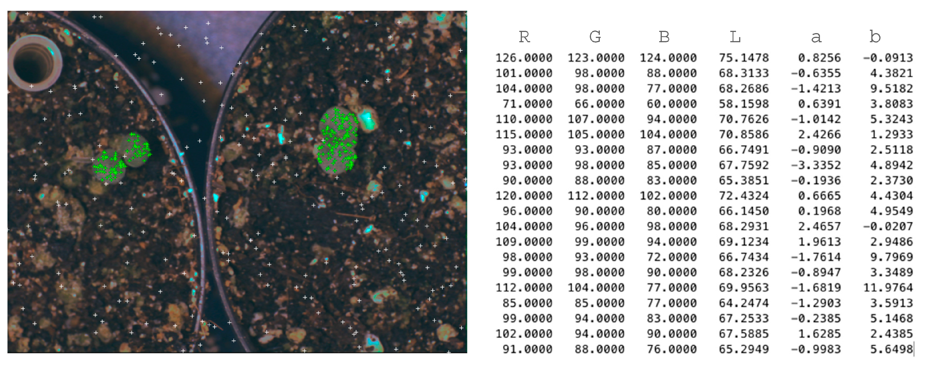
2.3.1. Extraction of Samples of Images Representative from the Different Classes
2.3.2. Features Vector
Colour Images
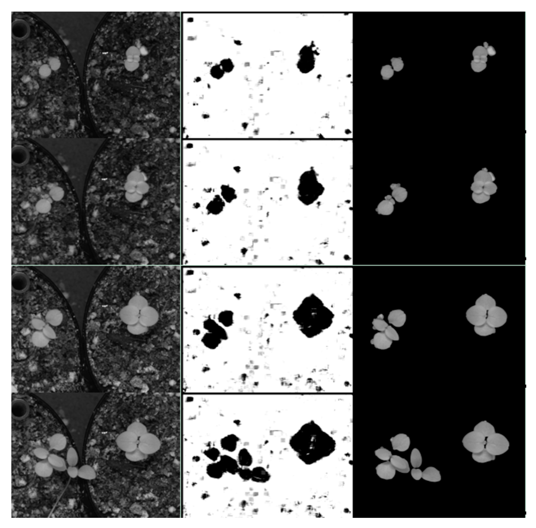
NIR Images
2.3.3. Classification Process
2.4. Experimental Validation
3. Results and Discussion
3.1. LOOCV
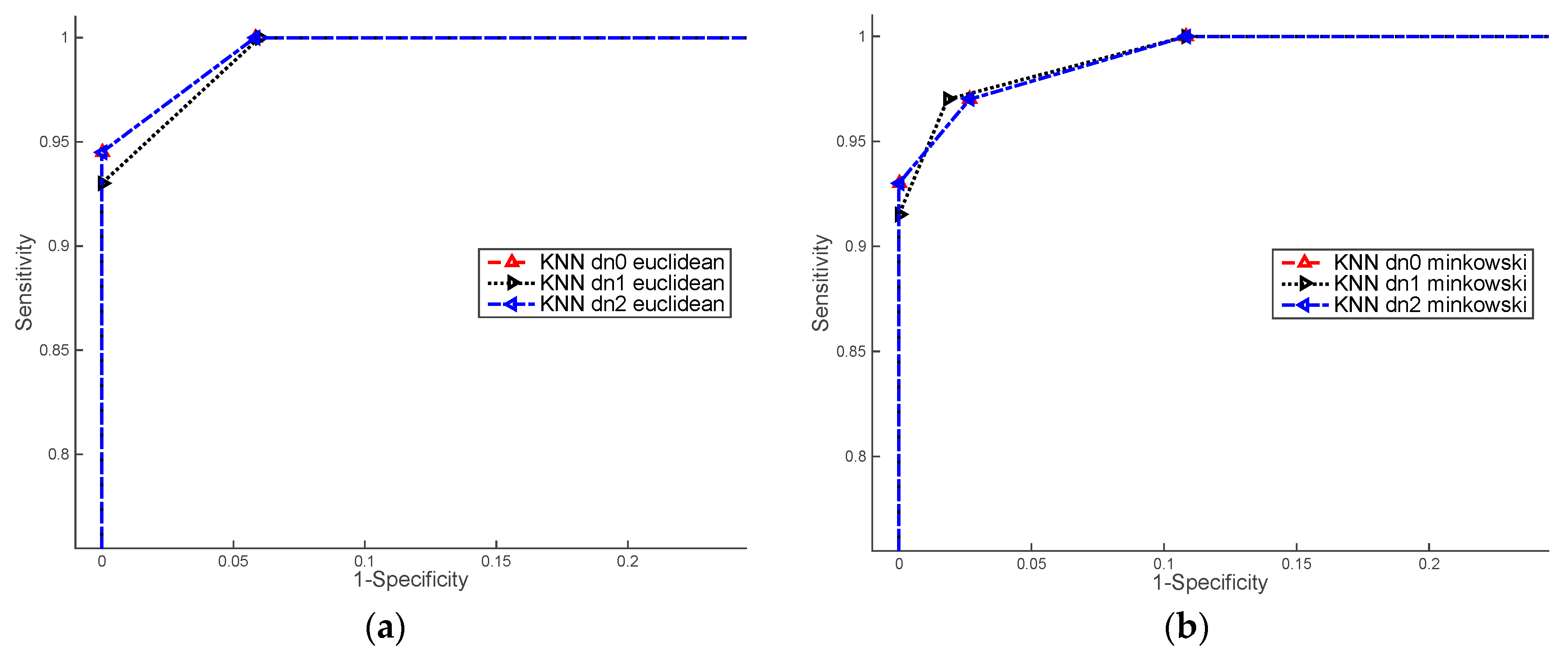
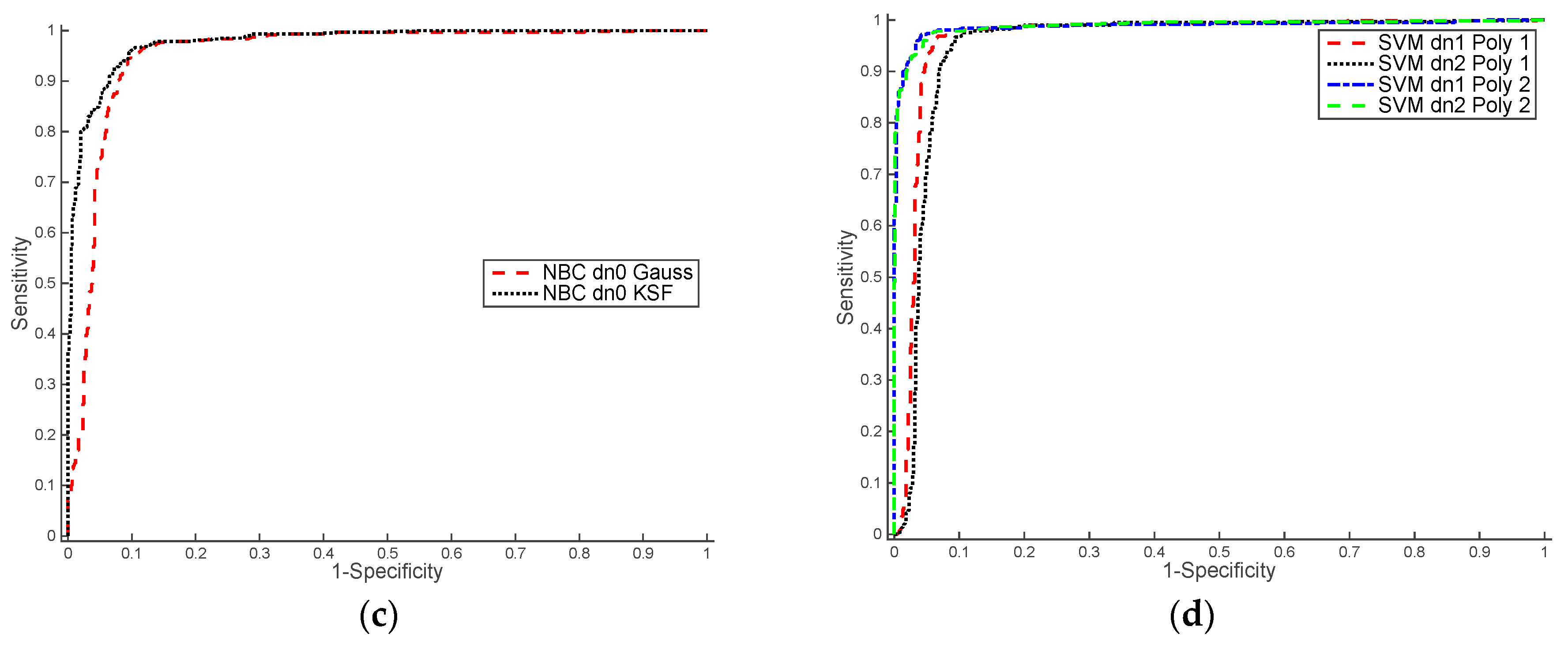
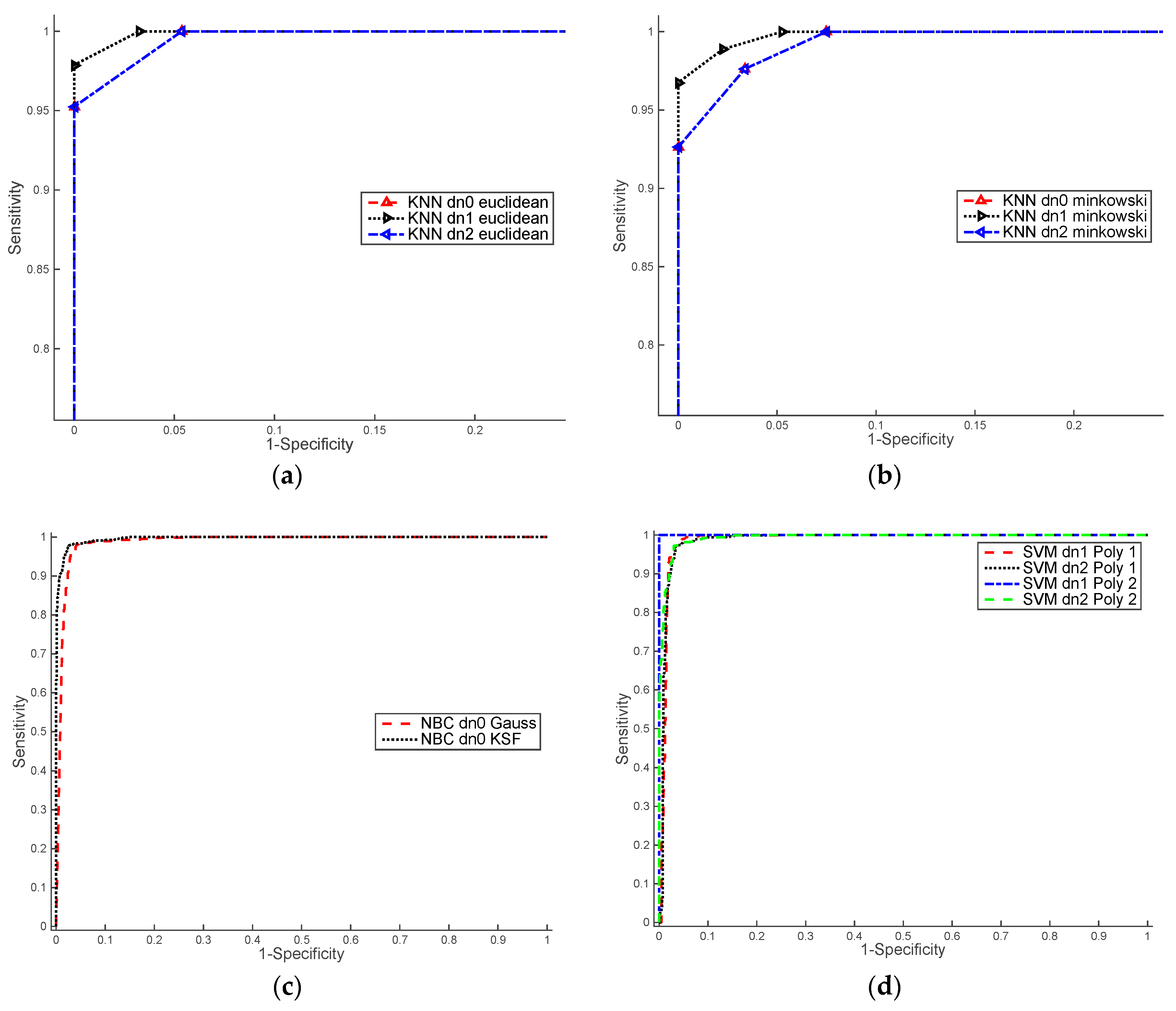
3.2. ROC Curves
3.3. Error Segmentation
4. Conclusions and Future Work
Acknowledgments
Author Contributions
Conflicts of Interest
Abbreviations
| LM | Machine learning |
| KSF | Kernel smoothing function |
| kNN | k-nearest neighbour |
| NBC | Naïve Bayes classifier |
| SVM | Support vector machines |
| LOOCV | Leave-one-out cross validation method |
| AUC | Area under curve |
| ME | Misclassification error |
References
- Fahlgren, N.; Gehan, M.; Baxter, I. Lights, camera, action: High-throughput plant phenotyping is ready for a close-up. Curr. Opin. Plant Biol. 2015, 24, 93–99. [Google Scholar] [CrossRef] [PubMed]
- Deligiannidis, L.; Arabnia, H. Emerging Trends in Image Processing, Computer Vision and Pattern Recognition; Elsevier: Boston, MA, USA, 2014. [Google Scholar]
- Dee, H.; French, A. From image processing to computer vision: Plant imaging grows up. Funct. Plant Biol. 2015, 42, iii–v. [Google Scholar] [CrossRef]
- Furbank, R.T.; Tester, M. Phenomics—Technologies to relieve the phenotyping bottleneck. Trends Plant Sci. 2011, 16, 635–644. [Google Scholar] [CrossRef] [PubMed]
- Dhondt, S.; Wuyts, N.; Inzé, D. Cell to whole-plant phenotyping: The best is yet to come. Trends Plant Sci. 2013, 18, 428–439. [Google Scholar] [CrossRef] [PubMed]
- Tisné, S.; Serrand, Y.; Bach, L.; Gilbault, E.; Ben Ameur, R.; Balasse, H.; Voisin, R.; Bouchez, D.; Durand-Tardif, M.; Guerche, P.; et al. Phenoscope: An automated large-scale phenotyping platform offering high spatial homogeneity. Plant J. 2013, 74, 534–544. [Google Scholar] [CrossRef] [PubMed]
- Li, L.; Zhang, Q.; Huang, D. A review of imaging techniques for plant phenotyping. Sensors 2014, 14, 20078–20111. [Google Scholar] [CrossRef] [PubMed]
- Honsdorf, N.; March, T.J.; Berger, B.; Tester, M.; Pillen, K. High-throughput phenotyping to detect drought tolerance QTL in wild barley introgression lines. PLoS ONE 2014, 9, 1–13. [Google Scholar] [CrossRef] [PubMed]
- Barron, J.; Liptay, A. Measuring 3-D plant growth using optical flow. Bioimaging 1997, 5, 82–86. [Google Scholar] [CrossRef]
- Aboelela, A.; Liptay, A.; Barron, J.L. Plant growth measurement techniques using near-infrared imagery. Int. J. Robot. Autom. 2005, 20, 42–49. [Google Scholar] [CrossRef]
- Navarro, P.J.; Fernández, C.; Weiss, J.; Egea-Cortines, M. Development of a configurable growth chamber with a computer vision system to study circadian rhythm in plants. Sensors 2012, 12, 15356–15375. [Google Scholar] [CrossRef] [PubMed]
- Nguyen, T.; Slaughter, D.; Max, N.; Maloof, J.; Sinha, N. Structured light-based 3d reconstruction system for plants. Sensors 2015, 15, 18587–18612. [Google Scholar] [CrossRef] [PubMed]
- Spalding, E.P.; Miller, N.D. Image analysis is driving a renaissance in growth measurement. Curr. Opin. Plant Biol. 2013, 16, 100–104. [Google Scholar] [CrossRef] [PubMed]
- Navlakha, S.; Bar-joseph, Z. Algorithms in nature: The convergence of systems biology and computational thinking. Mol. Syst. Biol. 2011, 7. [Google Scholar] [CrossRef] [PubMed]
- Kircher, M.; Stenzel, U.; Kelso, J. Improved base calling for the Illumina Genome Analyzer using machine learning strategies. Genome Biol. 2009, 10, 1–9. [Google Scholar] [CrossRef] [PubMed]
- Horton, P.; Nakai, K. Better prediction of protein cellular localization sites with the k nearest neighbors classifier. Proc. Int. Conf. Intell. Syst. Mol. Biol. 1997, 5, 147–152. [Google Scholar] [PubMed]
- Yousef, M.; Nebozhyn, M.; Shatkay, H.; Kanterakis, S.; Showe, L.C.; Showe, M.K. Combining multi-species genomic data for microRNA identification using a Naive Bayes classifier. Bioinformatics 2006, 22, 1325–1334. [Google Scholar] [CrossRef] [PubMed]
- Tellaeche, A.; Pajares, G.; Burgos-Artizzu, X.P.; Ribeiro, A. A computer vision approach for weeds identification through Support Vector Machines. Appl. Soft Comput. J. 2011, 11, 908–915. [Google Scholar] [CrossRef] [Green Version]
- Guerrero, J.M.; Pajares, G.; Montalvo, M.; Romeo, J.; Guijarro, M. Support Vector Machines for crop/weeds identification in maize fields. Expert Syst. Appl. 2012, 39, 11149–11155. [Google Scholar] [CrossRef]
- Covington, M.F.; Harmer, S.L. The circadian clock regulates auxin signaling and responses in Arabidopsis. PLoS Biol. 2007, 5, 1773–1784. [Google Scholar] [CrossRef] [PubMed]
- Nusinow, D.A.; Helfer, A.; Hamilton, E.E.; King, J.J.; Imaizumi, T.; Schultz, T.F.; Farré, E.M.; Kay, S.A.; Farre, E.M. The ELF4-ELF3-LUX complex links the circadian clock to diurnal control of hypocotyl growth. Nature 2011, 475, 398–402. [Google Scholar] [CrossRef] [PubMed]
- De Montaigu, A.; Toth, R.; Coupland, G. Plant development goes like clockwork. Trends Genet. 2010, 26, 296–306. [Google Scholar] [CrossRef] [PubMed]
- Baudry, A.; Ito, S.; Song, Y.H.; Strait, A.A.; Kiba, T.; Lu, S.; Henriques, R.; Pruneda-Paz, J.L.; Chua, N.H.; Tobin, E.M.; et al. F-box proteins FKF1 and LKP2 Act in concert with ZEITLUPE to control arabidopsis clock progression. Plant Cell 2010, 22, 606–622. [Google Scholar] [CrossRef] [PubMed]
- Kim, W.-Y.Y.; Fujiwara, S.; Suh, S.-S.S.; Kim, J.; Kim, Y.; Han, L.Q.; David, K.; Putterill, J.; Nam, H.G.; Somers, D.E. ZEITLUPE is a circadian photoreceptor stabilized by GIGANTEA in blue light. Nature 2007, 449, 356–360. [Google Scholar] [CrossRef] [PubMed]
- Khanna, R.; Kikis, E.A.; Quail, P.H. EARLY FLOWERING 4 functions in phytochrome B-regulated seedling de-etiolation. Plant Physiol. 2003, 133, 1530–1538. [Google Scholar] [CrossRef] [PubMed]
- Wenden, B.; Kozma-Bognar, L.; Edwards, K.D.; Hall, A.J.W.; Locke, J.C.W.; Millar, A.J. Light inputs shape the Arabidopsis circadian system. Plant J. 2011, 66, 480–491. [Google Scholar] [CrossRef] [PubMed]
- Nozue, K.; Covington, M.F.; Duek, P.D.; Lorrain, S.; Fankhauser, C.; Harmer, S.L.; Maloof, J.N. Rhythmic growth explained by coincidence between internal and external cues. Nature 2007, 448, 358–363. [Google Scholar] [CrossRef] [PubMed]
- Fernandez, C.; Suardiaz, J.; Jimenez, C.; Navarro, P.J.; Toledo, A.; Iborra, A. Automated visual inspection system for the classification of preserved vegetables. In Proceedings of the 2002 IEEE International Symposium on Industrial Electronics, ISIE 2002, Roma, Italy, 8–11 May 2002; pp. 265–269.
- Chen, Y.Q.; Nixon, M.S.; Thomas, D.W. Statistical geometrical features for texture classification. Pattern Recognit. 1995, 28, 537–552. [Google Scholar] [CrossRef]
- Haralick, R.M.; Shanmugam, K.; Dinstein, I.H. Textural features for image classification. IEEE Trans. Syst. Man Cybern. 1973, 610–621. [Google Scholar] [CrossRef]
- Zucker, S.W.; Terzopoulos, D. Finding structure in co-occurrence matrices for texture analysis. Comput. Graph. Image Process. 1980, 12, 286–308. [Google Scholar] [CrossRef]
- Bharati, M.H.; Liu, J.J.; MacGregor, J.F. Image texture analysis: Methods and comparisons. Chemom. Intell. Lab. Syst. 2004, 72, 57–71. [Google Scholar] [CrossRef]
- Navarro, P.J.; Alonso, D.; Stathis, K. Automatic detection of microaneurysms in diabetic retinopathy fundus images using the L*a*b color space. J. Opt. Soc. Am. A Opt. Image Sci. Vis. 2016, 33, 74–83. [Google Scholar] [CrossRef] [PubMed]
- Mallat, S.G. A theory for multiresolution signal decomposition: The wavelet representation. IEEE Trans. Pattern Anal. Mach. Intell. 1989, 11, 674–693. [Google Scholar] [CrossRef]
- Ghazali, K.H.; Mansor, M.F.; Mustafa, M.M.; Hussain, A. Feature extraction technique using discrete wavelet transform for image classification. In Proceedings of the 2007 5th Student Conference on Research and Development, Selangor, Malaysia, 11–12 December 2007; pp. 1–4.
- Arivazhagan, S.; Ganesan, L. Texture classification using wavelet transform. Pattern Recognit. Lett. 2003, 24, 1513–1521. [Google Scholar] [CrossRef]
- Lantz, B. Machine Learning with R; Packt Publishing Ltd.: Birmingham, UK, 2013. [Google Scholar]
- Hastie, T.; Tibshirani, R.; Friedman, J. The elements of statistical learning. Elements 2009, 1, 337–387. [Google Scholar]
- Bradley, A. The use of the area under the ROC curve in the evaluation of machine learning algorithms. Pattern Recognit. 1997, 30, 1145–1159. [Google Scholar] [CrossRef] [Green Version]
- Hand, D.J. Measuring classifier performance: A coherent alternative to the area under the ROC curve. Mach. Learn. 2009, 77, 103–123. [Google Scholar] [CrossRef]
- Sezgin, M.; Sankur, B. Survey over image thresholding techniques and quantitative performance evaluation. J. Electron. Imaging 2004, 13, 146–168. [Google Scholar]


| Configuration | kNN | NBC | SVM |
|---|---|---|---|
| method | Euclidean, Minkowski | Gauss, KSF | Linear, quadratic |
| data normalisation | dn0, dn1, dn2 | dn0 | dn1, dn2 |
| metrics | LOOCV, ROC | LOOCV, ROC | LOOCV, ROC |
| classes | 2 | 2 | 2 |
| Classifier | kNN | NBC | SVM | ||||
|---|---|---|---|---|---|---|---|
| Configuration | Euclidean | Minkowski | Gauss | KSF | Linear | Quadratic | |
| Colour | dn0 | 0.0283 | 0.0433 | 0.0750 | 0.0758 | - | - |
| dn1 | 0.0242 | 0.0467 | - | - | 0.0533 | 0.0383 | |
| dn2 | 0.0283 | 0.0433 | - | - | 0.0667 | 0.0450 | |
| NIR | dn0 | 0.0288 | 0.0394, | 0.0356 | 0.0319 | - | - |
| dn1 | 0.0169 | 0.0281 | - | - | 0.0326 | 0.0319 | |
| dn2 | 0.0288 | 0.0394 | - | - | 0.0344 | 0.0325 | |
| Classifier | kNN | NBC | SVM | ||||
|---|---|---|---|---|---|---|---|
| Configuration | Euclidean | Minkowski | Gauss | KSF | Linear | Quadratic | |
| Colour | dn0 | 0.9984 | 0.9974 | 0.9542 | 0.9778 | - | - |
| dn1 | 0.9979 | 0.9976 | - | - | 0.9622 | 0.9875 | |
| dn2 | 0.9984 | 0.9974 | - | - | 0.9496 | 0.9886 | |
| NIR | dn0 | 0.9987 | 0.9979 | 0.9877 | 0.9963 | - | - |
| dn1 | 0.9975 | 0.9993 | - | - | 0.9867 | 1.000 | |
| dn2 | 0.9987 | 0.9979 | - | - | 0.9868 | 0.9932 | |
| Classifier | kNN | SVM |
|---|---|---|
| Performance | 99.311% | 99.342% |
© 2016 by the authors; licensee MDPI, Basel, Switzerland. This article is an open access article distributed under the terms and conditions of the Creative Commons Attribution (CC-BY) license (http://creativecommons.org/licenses/by/4.0/).
Share and Cite
Navarro, P.J.; Pérez, F.; Weiss, J.; Egea-Cortines, M. Machine Learning and Computer Vision System for Phenotype Data Acquisition and Analysis in Plants. Sensors 2016, 16, 641. https://0-doi-org.brum.beds.ac.uk/10.3390/s16050641
Navarro PJ, Pérez F, Weiss J, Egea-Cortines M. Machine Learning and Computer Vision System for Phenotype Data Acquisition and Analysis in Plants. Sensors. 2016; 16(5):641. https://0-doi-org.brum.beds.ac.uk/10.3390/s16050641
Chicago/Turabian StyleNavarro, Pedro J., Fernando Pérez, Julia Weiss, and Marcos Egea-Cortines. 2016. "Machine Learning and Computer Vision System for Phenotype Data Acquisition and Analysis in Plants" Sensors 16, no. 5: 641. https://0-doi-org.brum.beds.ac.uk/10.3390/s16050641