Segmentation of Gait Sequences in Sensor-Based Movement Analysis: A Comparison of Methods in Parkinson’s Disease

 , ,
, ,
Abstract
:1. Introduction
2. Methods
2.1. Peak Detection
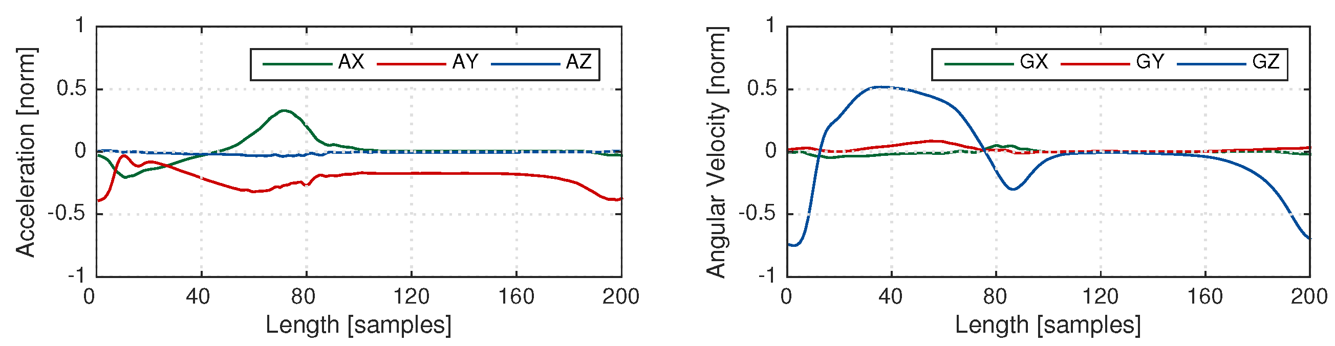
2.2. Multi-subsequence Dynamic Time Warping
- Distance matrix : The elements of represent the pairwise distance between the elements of the template X and the gait sequence Y. The size of the matrix is . In the case of including several axes, separate distance matrices are computed and they are all summed up to construct a single distance matrix [33].
- Accumulated cost matrix : represents the distance between the template and the gait sequence as well as the accumulated costs of warping the template to parts of the gait sequence. The bottom row of matrix is as follows:The first column is:The remaining elements are calculated in a recursive manner as
- Distance function : The top row of matrix represents the accumulated costs for warping the stride template X to the gait sequence Y and can be considered as a matching function .
- Warping path P: Warping path of length L with elements for presents a good match between X and Y. Local minimums of the matching function are considered as the end points of warping paths and starting points are obtained by backtracking on the accumulated cost matrix. A threshold should be chosen in order to select these local minimums in such a way to find the maximum number of relevant strides in the sequence.
- Boundary conditions for a complete stride:
- Start of warping path P is in the top row of the cost matrix .
- End of warping path P is in the bottom row of cost matrix .
- Condition to ensure warping path monotonically decreases:
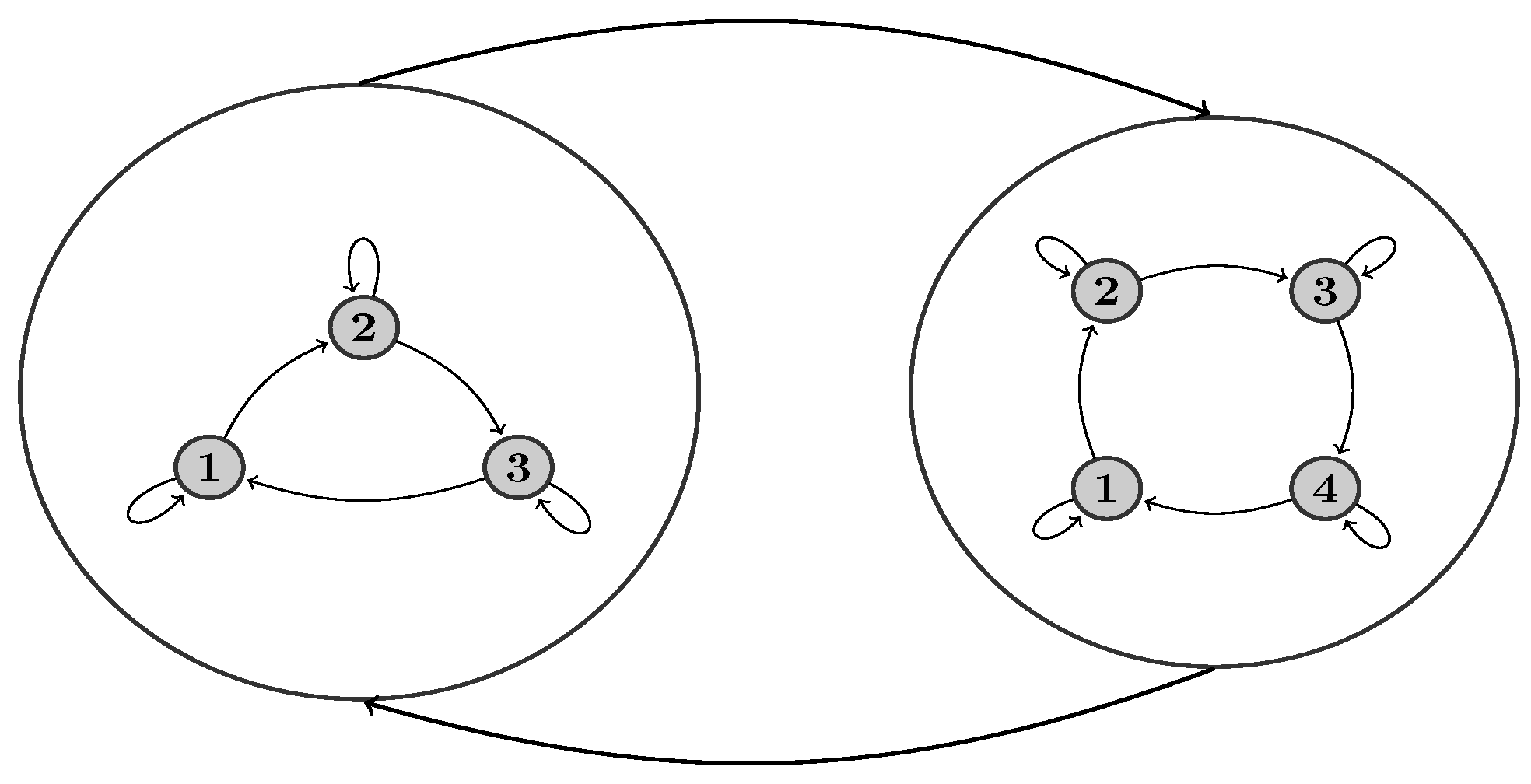
2.3. Hierarchical Hidden Markov Models
3. Evaluation Study
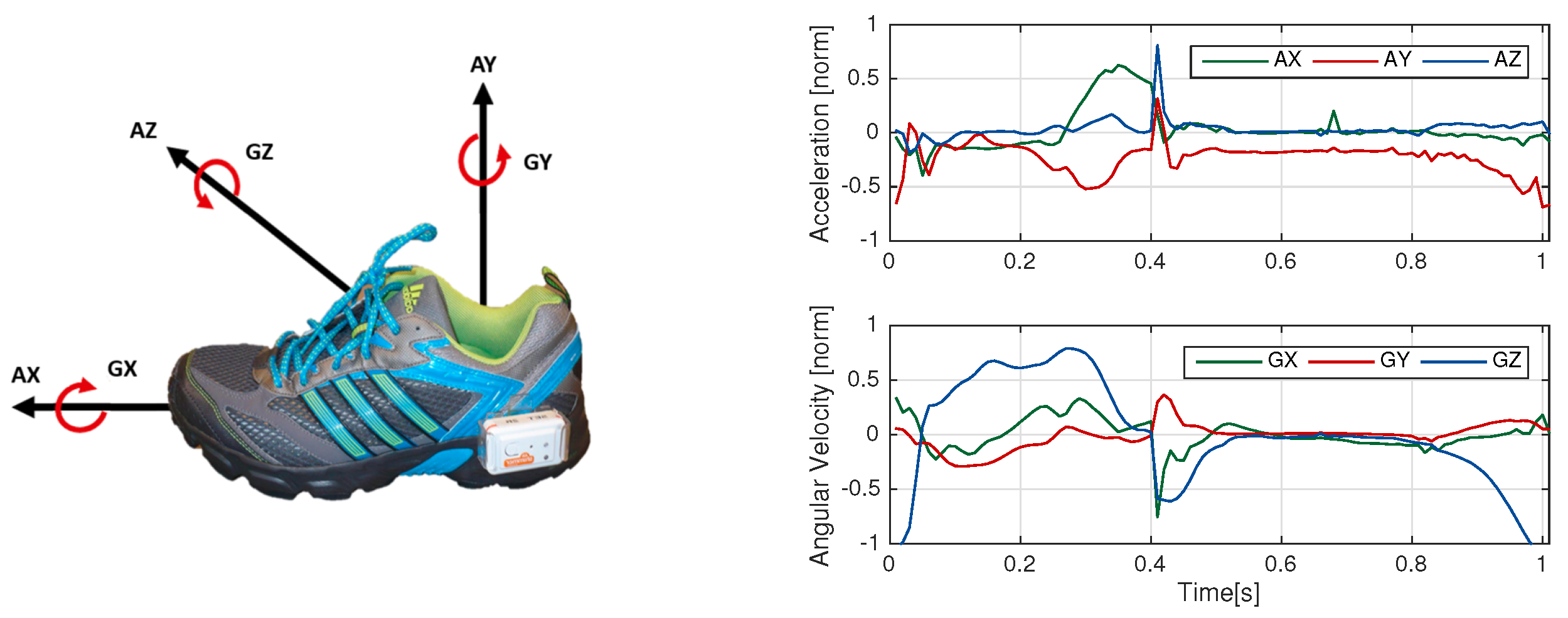
3.1. Data Collection and Setup
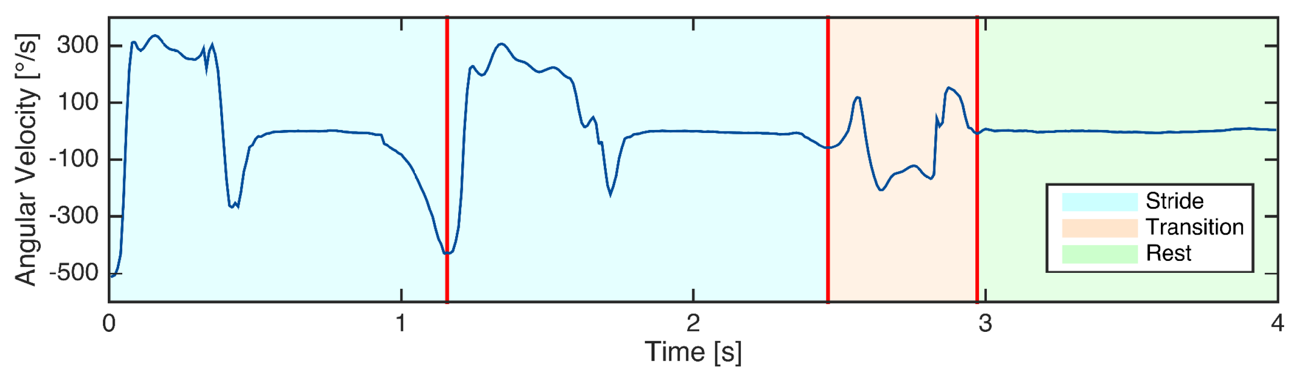
3.2. Manual Data Labeling
3.3. Implementation of Peak Detection
3.4. Implementation of Euclidean DTW
3.5. Implementation of Probabilistic DTW
3.6. Implementation of hHMM
3.7. Performance Assessment
4. Experimental Results
5. Discussion and Conclusion
Acknowledgments
Author Contributions
Conflicts of Interest
References
- Parkinson, J. An Essay on the Shaking Palsy; Neely & Jones: London, UK, 1817. [Google Scholar]
- Hoehn, M.M.; Yahr, M.D. Parkinsonism: Onset, progression and mortality. Neurology 1967, 17, 427–442. [Google Scholar] [CrossRef] [PubMed]
- Goetz, C.G.; Tilley, B.C.; Shaftman, S.R.; Stebbins, G.T.; Fahn, S.; Martinez-Martin, P.; Poewe, W.; Sampaio, C.; Stern, M.B.; Dodel, R.; et al. Movement Disorder Society-sponsored revision of the Unified Parkinson’s Disease Rating Scale (MDS-UPDRS): Scale presentation and clinimetric testing results. Movement Disord. 2008, 23, 2129–2170. [Google Scholar] [CrossRef] [PubMed]
- Podsiadlo, D.; Richardson, S. The timed “Up & Go”: A test of basic functional mobility for frail elderly persons. J. Am. Geriatr. Soc. 1991, 39, 142–148. [Google Scholar] [PubMed]
- Marchese, R.; Bove, M.; Abbruzzese, G. Effect of cognitive and motor tasks on postural stability in Parkinson’s disease: A posturographic study. Movement Disord. 2003, 18, 652–658. [Google Scholar] [CrossRef] [PubMed]
- Richards, M.; Marder, K.; Cote, L.; Mayeux, R. Interrater reliability of the unified Parkinson’s disease rating scale motor examination. Movement Disord. Jan 1994, 9, 89–91. [Google Scholar] [CrossRef] [PubMed]
- Maetzler, W.; Klucken, J.; Horne, M. A clinical view on the development of technology-based tools in managing Parkinson’s disease. Movement Disord. 2016, 31, 1263–1271. [Google Scholar] [CrossRef] [PubMed]
- Klucken, J.; Friedl, K.; Eskofier, B.M.; Hausdorf, J.M. Guest Editorial: Enabling Technologies for Parkinson’s Disease Management. IEEE J. Biomed. Health Inform. 2015, 19, 1775–1776. [Google Scholar] [CrossRef] [PubMed]
- Espay, A.J.; Bonato, P.; Nahab, F.B.; Maetzler, W.; Dean, J.M.; Klucken, J.; Eskofier, B.M.; Merola, A.; Horak, F.; Lang, A.E.; et al. Technology in Parkinson’s disease: Challenges and opportunities. Movement Disord. 2016, 31, 1272–1282. [Google Scholar] [CrossRef] [PubMed]
- Gray, P.; Hildebrand, K. Fall risk factors in Parkinson’s disease. J. Neurosci. Nurs. 2000, 32, 222–228. [Google Scholar] [CrossRef] [PubMed]
- Schrag, A.; Jahanshahi, M.; Quinn, N. How does Parkinson’s disease affect quality of life? A comparison with quality of life in the general population. Movement Disord. 2000, 15, 1112–1118. [Google Scholar] [CrossRef]
- Salarian, A.; Russmann, H.; Vingerhoets, F.J.; Dehollain, C.; Blanc, Y.; Burkhard, P.R.; Aminian, K. Gait assessment in Parkinson’s disease: Toward an ambulatory system for long-term monitoring. IEEE Trans. Biomed. Eng. 2004, 51, 1434–1443. [Google Scholar] [CrossRef] [PubMed]
- Chen, B.R.; Patel, S.; Buckley, T.; Rednic, R.; McClure, D.J.; Shih, L.; Tarsy, D.; Welsh, M.; Bonato, P. A web-based system for home monitoring of patients with Parkinson’s disease using wearable sensors. IEEE Trans. Biomed. Eng. 2011, 58, 831–836. [Google Scholar] [CrossRef] [PubMed]
- Kluge, F.; Gaßner, H.; Hannink, J.; Pasluosta, C.; Klucken, J.; Eskofier, B.M. Towards Mobile Gait Analysis: Concurrent Validity and Test-Retest Reliability of an Inertial Measurement System for the Assessment of Spatio-Temporal Gait Parameters. Sensors 2017, 17, 1522. [Google Scholar] [CrossRef] [PubMed]
- Mariani, B.; Jiménez, M.C.; Vingerhoets, F.J.; Aminian, K. On-shoe wearable sensors for gait and turning assessment of patients with Parkinson’s disease. IEEE Trans. Biomed. Eng. 2013, 60, 155–158. [Google Scholar] [CrossRef] [PubMed]
- Pasluosta, C.F.; Gassner, H.; Winkler, J.; Klucken, J.; Eskofier, B.M. An emerging era in the management of Parkinson’s disease: Wearable technologies and the internet of things. IEEE J. Biomed. Health Inf. 2015, 19, 1873–1881. [Google Scholar] [CrossRef] [PubMed]
- Rampp, A.; Barth, J.; Schülein, S.; Gaßmann, K.G.; Klucken, J.; Eskofier, B.M. Inertial Sensor-Based Stride Parameter Calculation From Gait Sequences in Geriatric Patients. IEEE Trans. Biomed. Eng. 2015, 62, 1089–1097. [Google Scholar] [CrossRef] [PubMed]
- Hannink, J.; Kautz, T.; Pasluosta, C.; Barth, J.; Schulein, S.; Gassmann, K.G.; Klucken, J.; Eskofier, B. Mobile Stride Length Estimation with Deep Convolutional Neural Networks. IEEE J. Biomed. Health Inf. 2017. [Google Scholar] [CrossRef] [PubMed]
- Trojaniello, D.; Cereatti, A.; Pelosin, E.; Avanzino, L.; Mirelman, A.; Hausdorff, J.M.; Della Croce, U. Estimation of step-by-step spatio-temporal parameters of normal and impaired gait using shank-mounted magneto-inertial sensors: Application to elderly, hemiparetic, parkinsonian and choreic gait. J. Neuroeng. Rehabil. 2014, 11, 152. [Google Scholar] [CrossRef] [PubMed]
- Kang, H.G.; Dingwell, J.B. Separating the effects of age and walking speed on gait variability. Gait Posture 2008, 27, 572–577. [Google Scholar] [CrossRef] [PubMed]
- Kluge, F.; Krinner, S.; Lochmann, M.; Eskofier, B.M. Speed dependent effects of laterally wedged insoles on gait biomechanics in healthy subjects. Gait Posture 2017, 55, 145–149. [Google Scholar] [CrossRef] [PubMed]
- Agostini, V.; Balestra, G.; Knaflitz, M. Segmentation and classification of gait cycles. IEEE Trans. Neur. Syst. Rehabil. Eng. 2014, 22, 946–952. [Google Scholar] [CrossRef] [PubMed]
- Agostini, V.; Gastaldi, L.; Rosso, V.; Knaflitz, M.; Tadano, S. A Wearable Magneto-Inertial System for Gait Analysis (H-Gait): Validation on Normal Weight and Overweight/Obese Young Healthy Adults. Sensors 2017, 17, 2406. [Google Scholar] [CrossRef] [PubMed]
- Selles, R.W.; Formanoy, M.A.G.; Bussmann, J.B.J.; Janssens, P.J.; Stam, H.J. Automated Estimation of Initial and Terminal Contact Timing Using Accelerometers; Development and Validation in Transtibial Amputees and Controls. IEEE Trans. Neur. Syst. Rehabil. Eng. 2005, 13, 81–88. [Google Scholar] [CrossRef] [PubMed]
- Derawi, M.O.; Bours, P.; Holien, K. Improved Cycle Detection for Accelerometer Based Gait Authentication. In Proceedings of the Sixth International Conference on Intelligent Information Hiding and Multimedia Signal Processing, Darmstadt, Germany, 15–17 October 2010. [Google Scholar]
- Libby, R. A Simple Method for Reliable Footstep Detection on Embedded Sensor Platforms. 2008. Available online: https://www.researchgate.net/publication/265189201_A_simple_method_for_reliable_footstep_detection_on_embedded_sensor_platforms (accessed on 6 January 2018).
- Hundza, S.R.; Hook, W.R.; Harris, C.R.; Mahajan, S.V.; Leslie, P.A.; Spani, C.A.; Spalteholz, L.G.; Birch, B.J.; Commandeur, D.T.; Livingston, N.J. Accurate and reliable gait cycle detection in Parkinson’s disease. IEEE Trans. Neur. Syst. Rehabil. Eng. 2014, 22, 127–137. [Google Scholar] [CrossRef] [PubMed]
- Aminian, K.; Najafi, B.; Büla, C.; Leyvraz, P.F.; Robert, P. Spatio-temporal parameters of gait measured by an ambulatory system using miniature gyroscopes. J. Biomech. 2002, 35, 689–699. [Google Scholar] [CrossRef]
- Khandelwal, S.; Wickstrom, N. Identification of Gait Events using Expert Knowledge and Continuous Wavelet Transform Analysis. In Proceedings of the International Conference on Bio-inspired Systems and Signal Processing, Angers, France, 3–6 March 2014; pp. 197–204. [Google Scholar]
- Gouwanda, D.; Senanayake, S.A. Application of hybrid multi-resolution wavelet decomposition method in detecting human walking gait events. In Proceedings of the International Conference of Soft Computing and Pattern Recognition, Malacca, Malaysia, 4–7 December 2009; pp. 580–585. [Google Scholar]
- Müller, M. Dynamic time warping. In Information Retrieval for Music and Motion; Springer: New York, NY, USA, 2007; pp. 69–84. [Google Scholar]
- ten Holt, G.A.; Reinders, M.J.; Hendriks, E.A. Multi-Dimensional Dynamic Time Warping for Gesture Recognition. In Proceedings of the Thirteenth annual conference of the Advanced School for Computing and Imaging, Heijen, The Netherlands, 13–15 June 2007. [Google Scholar]
- Barth, J.; Oberndorfer, C.; Pasluosta, C.; Schülein, S.; Gassner, H.; Reinfelder, S.; Kugler, P.; Schuldhaus, D.; Winkler, J.; Klucken, J.; et al. Stride segmentation during free walk movements using multi-dimensional subsequence dynamic time warping on inertial sensor data. Sensors 2015, 15, 6419–6440. [Google Scholar] [CrossRef] [PubMed]
- Mannini, A.; Sabatini, A.M. A hidden Markov model-based technique for gait segmentation using a foot-mounted gyroscope. In Proceedings of the 33th Annual International Conference of the IEEE Engineering in Medicine and Biology Society (EMBC), Boston, MA, USA, 30 Auguest–3 September 2011; pp. 4369–4373. [Google Scholar]
- Mannini, A.; Trojaniello, D.; Della Croce, U.; Sabatini, A.M. Hidden Markov model-based strategy for gait segmentation using inertial sensors: Application to elderly, hemiparetic patients and Huntington’s disease patients. In Proceedings of the 37th Annual International Conference of the IEEE Engineering in Medicine and Biology Society (EMBC), Milano, Italy, 25–29 August 2015; pp. 5179–5182. [Google Scholar]
- Panahandeh, G.; Mohammadiha, N.; Leijon, A.; Handel, P. Continuous Hidden Markov Model for Pedestrian Activity Classification and Gait Analysis. IEEE Trans. Instrum. Meas. 2013, 62, 1073–1083. [Google Scholar] [CrossRef]
- Pfau, T.; Ferrari, M.; Parsons, K.; Wilson, A. A hidden Markov model-based stride segmentation technique applied to equine inertial sensor trunk movement data. J. Biomech. 2008, 41, 216–220. [Google Scholar] [CrossRef] [PubMed]
- Martindale, C.F.; Strauss, M.; Gaßner, H.; List, J.; Müller, M.; Klucken, J.; Kohl, Z.; Eskofier, B.M. Segmentation of Gait Sequences using Inertial Sensor Data in Hereditary Spastic Paraplegia. In Proceedings of the International Conference of the IEEE Engineering in Medicine and Biology Society (EMBC), Jeju Island, Korea, 11–15 July 2017. [Google Scholar]
- El-Gohary, M.; Pearson, S.; McNames, J.; Mancini, M.; Horak, F.; Mellone, S.; Chiari, L. Continuous monitoring of turning in patients with movement disability. Sensors 2014, 14, 356–369. [Google Scholar] [CrossRef] [PubMed]
- Klucken, J.; Barth, J.; Kugler, P.; Schlachetzki, J.; Henze, T.; Marxreiter, F.; Kohl, Z.; Steidl, R.; Hornegger, J.; Eskofier, B.; Winkler, J. Unbiased and Mobile Gait Analysis Detects Motor Impairment in Parkinson’s Disease. PLoS ONE 2013, 8. [Google Scholar] [CrossRef] [PubMed]
- Bautista, M.; Hernandez-Vela, A.; Ponce, V.; Perez-Sala, X.; Bar, X.; Pujol, O.; Angulo, C.; Escalera, S. Probability-based Dynamic Time Warping for Gesture Recognition on RGB-D data. Adv. Depth Image Anal. Appl. 2013, 7854, 126–135. [Google Scholar]
- Rabiner, L.; Juang, B. An introduction to hidden Markov models. IEEE ASSP Mag. 1986, 3, 4–16. [Google Scholar] [CrossRef]
- Ghahramani, Z. An introduction to hidden Markov models and Bayesian networks. Int. J. Pattern Recogn. 2001, 15, 9–42. [Google Scholar] [CrossRef]
- Gales, M.; Young, S. The application of hidden Markov models in speech recognition. In Foundations and Trends in Signal Processing; Now Publishers Inc.: Hanover, MA, USA, 2008; Volume 1, pp. 195–304. [Google Scholar] [CrossRef]
- Lukashin, A.V.; Borodovsky, M. GeneMark.hmm: New solutions for gene finding. Nucleic Acids Res. 1998, 26, 1107–1115. [Google Scholar] [CrossRef] [PubMed]
- Fine, S.; Singer, Y.; Tishby, N. The hierarchical hidden Markov model: Analysis and applications. Mach. Learn. 1998, 32, 41–62. [Google Scholar] [CrossRef]
- Crenna, P.; Carpinella, I.; Rabuffetti, M.; Calabrese, E.; Mazzoleni, P.; Nemni, R.; Ferrarin, M. The association between impaired turning and normal straight walking in Parkinson’s disease. Gait posture 2007, 26, 172–178. [Google Scholar] [CrossRef] [PubMed]
- Bilmes, J.A. A Gentle Tutorial of the EM Algorithm and Its Application to Parameter Estimation for Gaussian Mixture and Hidden Markov Models; University of Berkeley: Berkeley, CA, USA, 1997. [Google Scholar]
- Dempster, A.P.; Laird, N.M.; Rubin, D.B. Maximum likelihood from incomplete data via the EM algorithm. J. R. Stat. Soc. Series B Methodol 1977, 1–38. [Google Scholar]
- Viterbi, A. Error bounds for convolutional codes and an asymptotically optimum decoding algorithm. IEEE Trans. Inf. Theory 1967, 13, 260–269. [Google Scholar] [CrossRef]
- Steidl, S.; Riedhammer, K.; Bocklet, T.; Florian, H.; Nöth, E. Java Visual Speech Components for Rapid Application Development of GUI based Speech Processing Applications. In Proceedings of the 12th Annual Conference of the International Speech Communication Association 2011 (INTERSPEECH 2011), Florence, Italy, 28–31 August 2011. [Google Scholar]
- Mannini, A.; Sabatini, A.M. Gait phase detection and discrimination between walking–jogging activities using hidden Markov models applied to foot motion data from a gyroscope. Gait posture 2012, 36, 657–661. [Google Scholar] [CrossRef] [PubMed]
- Schlachetzki, J.C.; Barth, J.; Marxreiter, F.; Gossler, J.; Kohl, Z.; Reinfelder, S.; Gassner, H.; Aminian, K.; Eskofier, B.M.; Winkler, J.; et al. Wearable sensors objectively measure gait parameters in Parkinson’s disease. PLoS ONE 2017, 12, e0183989. [Google Scholar] [CrossRef] [PubMed]
- Gaßner, H.; Marxreiter, F.; Kohl, Z.; Schlachetzki, J.; Eskofier, B.; Winkler, J.; Klucken, J. Impaired gait parameters are more sensitive for dual task performance than cognitive impairment in Parkinson’s disease. Basal Ganglia 2017, 8, 3. [Google Scholar] [CrossRef]
- Zampieri, C.; Salarian, A.; Carlson-Kuhta, P.; Nutt, J.G.; Horak, F.B. Assessing mobility at home in people with early Parkinson’s disease using an instrumented Timed Up and Go test. Parkinsonism Relat. Disord. 2011, 17, 277–280. [Google Scholar] [CrossRef] [PubMed]
- Saito, N.; Yamamoto, T.; Sugiura, Y.; Shimizu, S.; Shimizu, M. Lifecorder: A new device for the long-term monitoring of motor activities for Parkinson’s disease. Intern. Med. 2004, 43, 685–692. [Google Scholar] [CrossRef] [PubMed]
- LeCun, Y.; Bengio, Y.; Hinton, G. Deep learning. Nature 2015, 521, 436–444. [Google Scholar] [CrossRef] [PubMed]
- Leggetter, C.J.; Woodland, P.C. Maximum likelihood linear regression for speaker adaptation of continuous density hidden Markov models. Comput. Speech Lang. 1995, 9, 171–185. [Google Scholar] [CrossRef]


| Signal Combination | GZ | AXGZ | AYGZ | AXAYGZ |
|---|---|---|---|---|
| Threshold (steps of 5) | 10–25 | 20–30 | 20–30 | 25–40 |
| Signal Combination | GZ | AXGZ | AYGZ | AXAYGZ |
|---|---|---|---|---|
| Threshold (steps of 1) | 8–15 | 8–15 | 8–15 | 8–15 |
| Parameters | Values |
|---|---|
| Sliding window length (s) (steps of 0.20) | 0.10–0.70 |
| Number of sub-states for stride | transition | rest (steps of 2) | 4–12 | 2–4 | 1 |
| Number of Gaussian mixture model (GMM) components (steps of 2) | 8–12 |
| Number of principal components (steps of 2) | 1–15 |
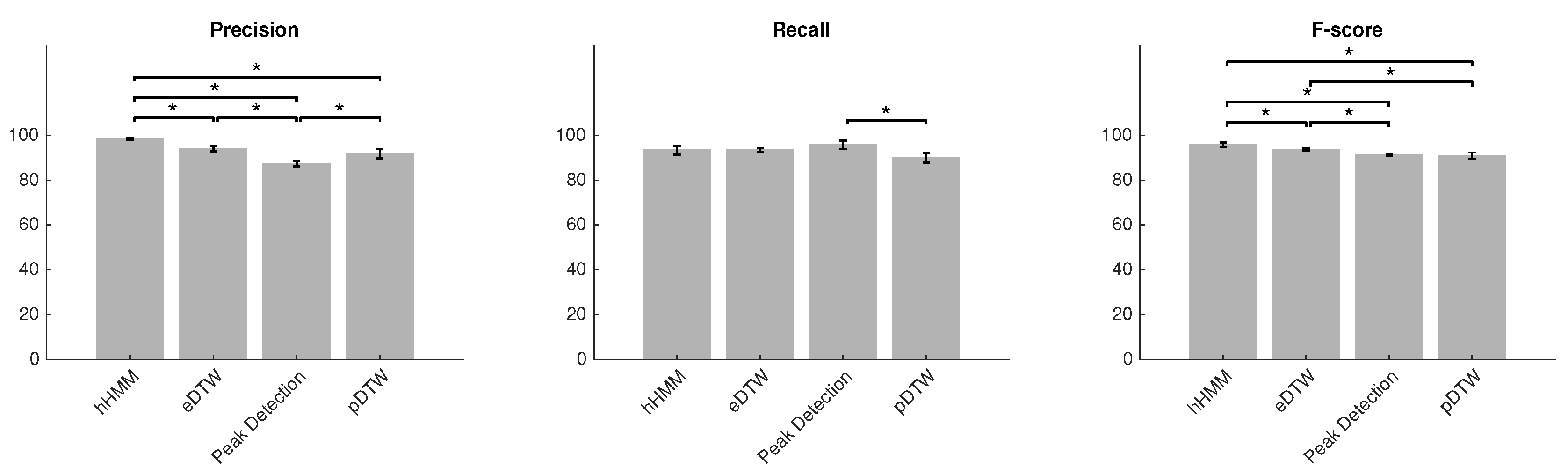
| Method | Precision (%) | Recall (%) | F-score (%) |
|---|---|---|---|
| hHMM | 98.5 ± 0.4 | 93.5 ± 1.9 | 95.9 ± 0.9 |
| eDTW | 94 ± 1.2 | 93.5 ± 0.8 | 93.8 ± 0.5 |
| Peak detection | 87.4 ± 1.2 | 95.9 ± 1.8 | 91.5 ± 0.4 |
| pDTW | 91.8 ± 2.1 | 90.1 ± 2.2 | 90.9 ± 1.4 |
© 2018 by the authors. Licensee MDPI, Basel, Switzerland. This article is an open access article distributed under the terms and conditions of the Creative Commons Attribution (CC BY) license (http://creativecommons.org/licenses/by/4.0/).
Share and Cite
Haji Ghassemi, N.; Hannink, J.; Martindale, C.F.; Gaßner, H.; Müller, M.; Klucken, J.; Eskofier, B.M. Segmentation of Gait Sequences in Sensor-Based Movement Analysis: A Comparison of Methods in Parkinson’s Disease. Sensors 2018, 18, 145. https://0-doi-org.brum.beds.ac.uk/10.3390/s18010145
Haji Ghassemi N, Hannink J, Martindale CF, Gaßner H, Müller M, Klucken J, Eskofier BM. Segmentation of Gait Sequences in Sensor-Based Movement Analysis: A Comparison of Methods in Parkinson’s Disease. Sensors. 2018; 18(1):145. https://0-doi-org.brum.beds.ac.uk/10.3390/s18010145
Chicago/Turabian StyleHaji Ghassemi, Nooshin, Julius Hannink, Christine F. Martindale, Heiko Gaßner, Meinard Müller, Jochen Klucken, and Björn M. Eskofier. 2018. "Segmentation of Gait Sequences in Sensor-Based Movement Analysis: A Comparison of Methods in Parkinson’s Disease" Sensors 18, no. 1: 145. https://0-doi-org.brum.beds.ac.uk/10.3390/s18010145