Accuracy of Trajectory Tracking Based on Nonlinear Guidance Logic for Hydrographic Unmanned Surface Vessels

 ,
,  ,
,
Abstract
:1. Introduction
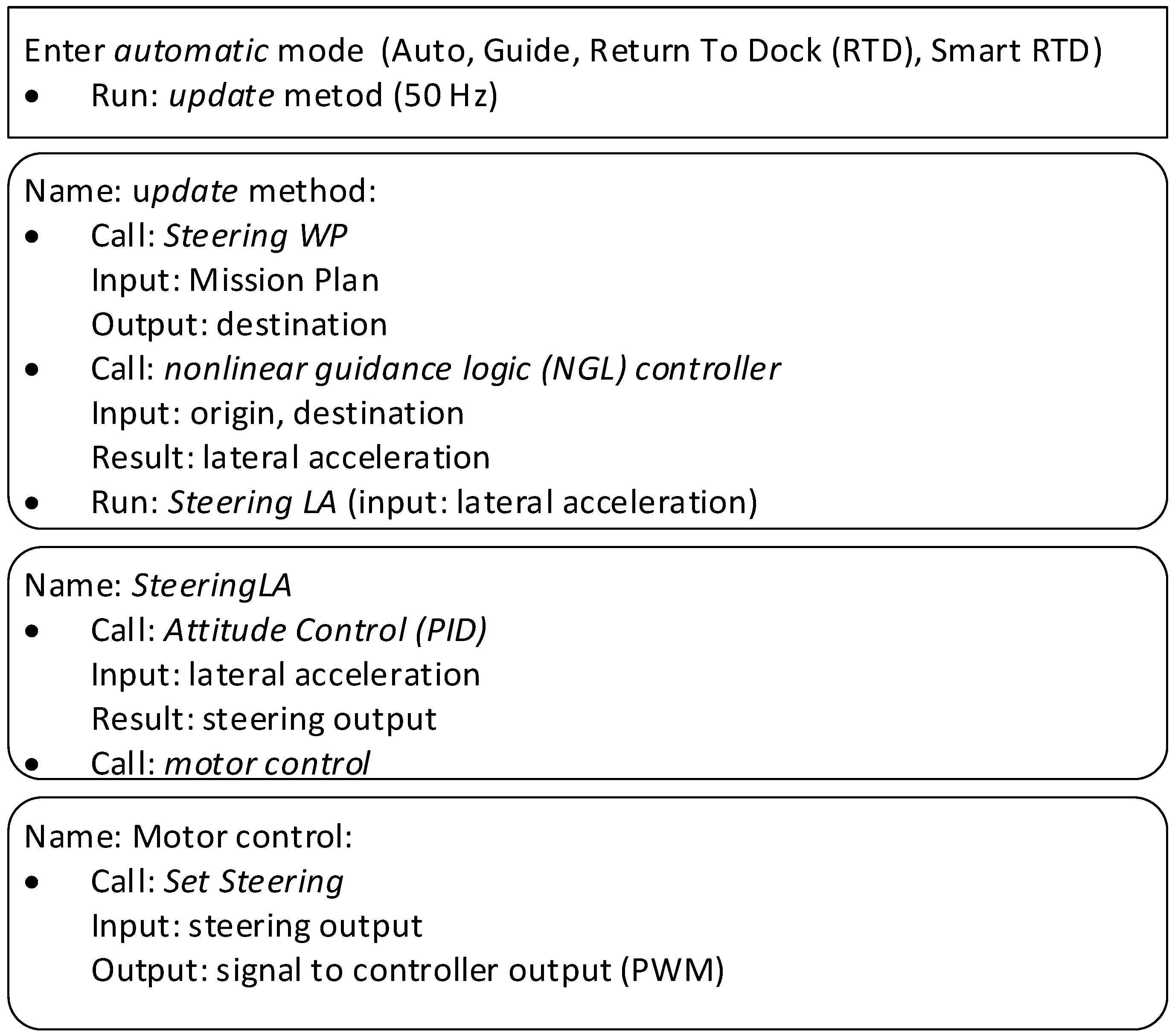
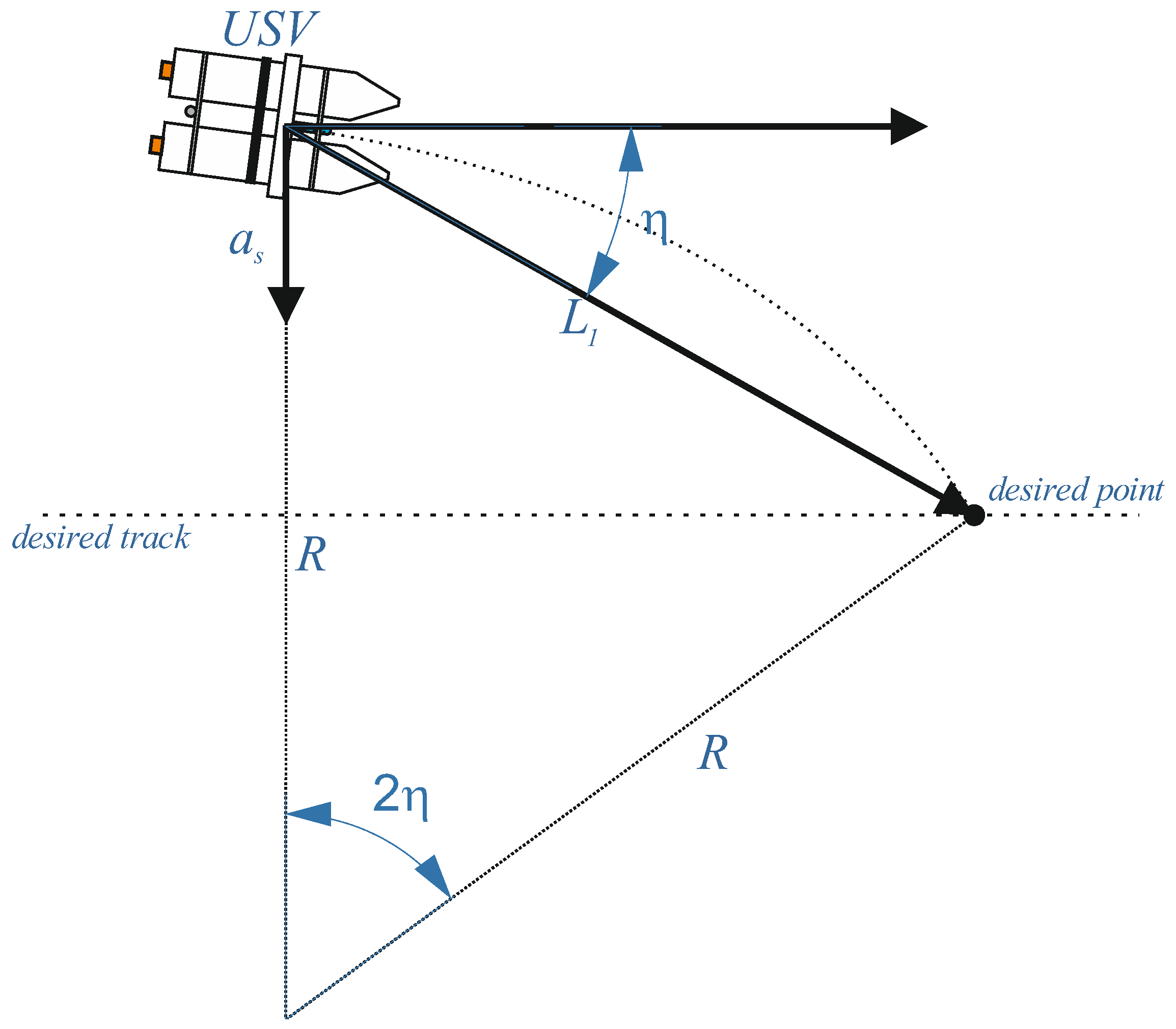
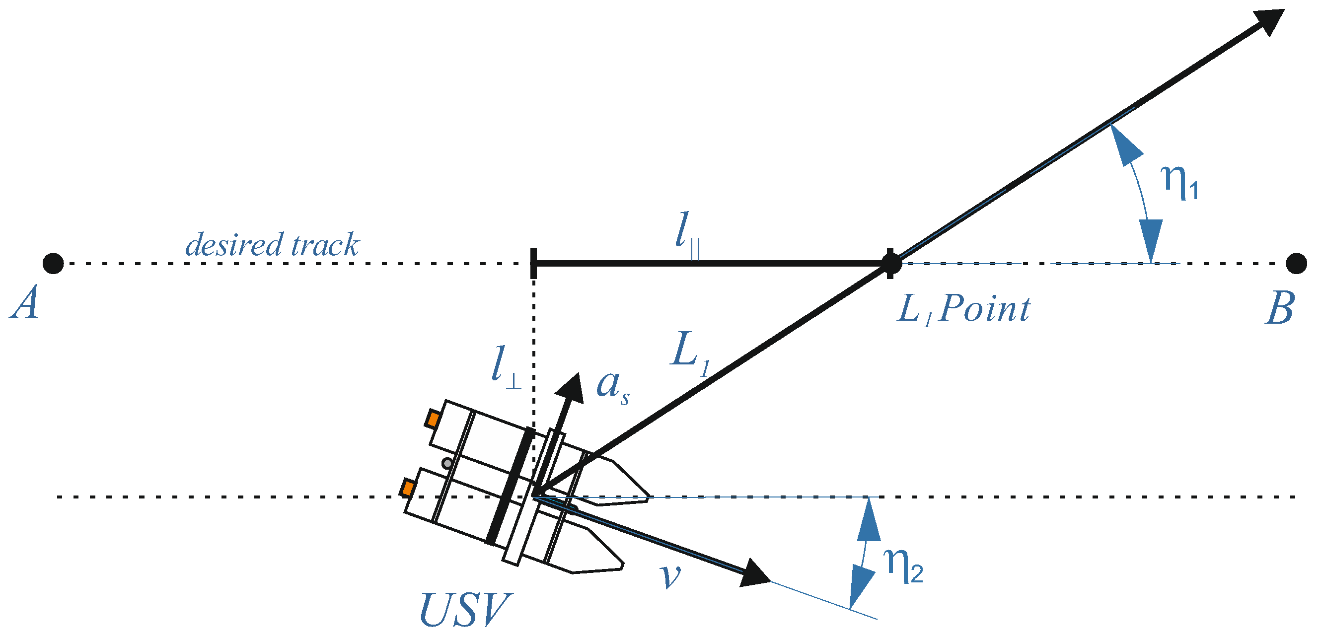
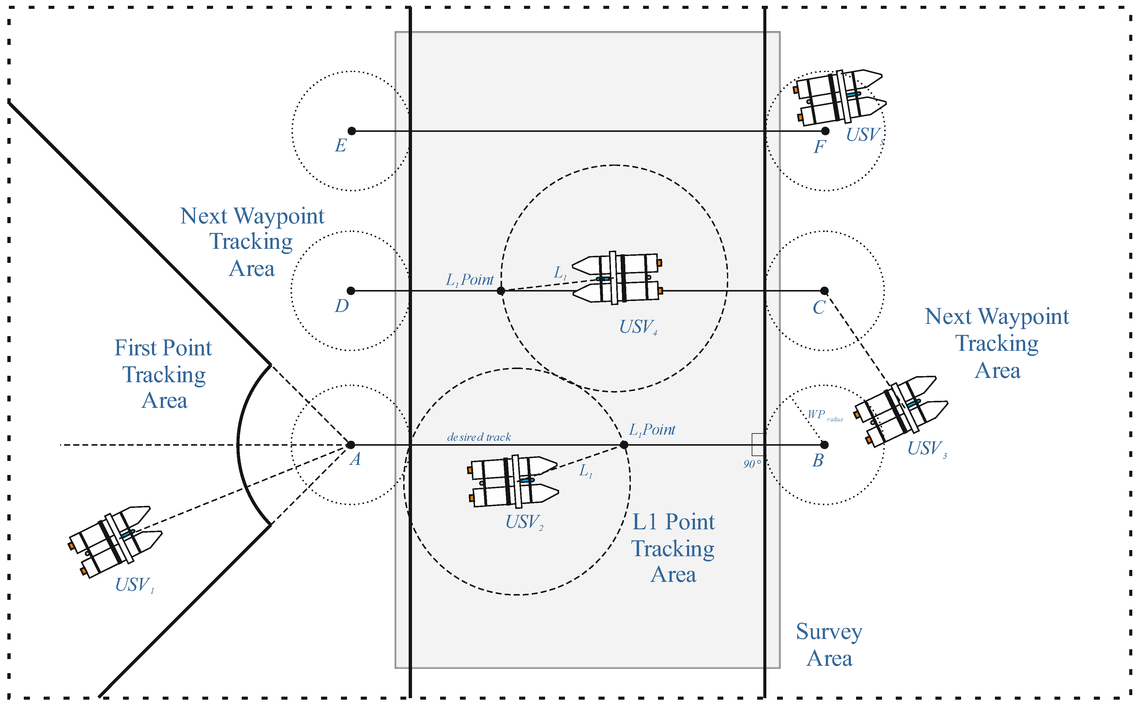
2. Trajectory Tracking
- Steering WP—the basic route plan and vehicle destination. The method provides the location that the vehicle should achieve (destination).
- NLG controller—the method where the navigation process is implemented. The method, based on destination and vehicle origin, calculates the lateral acceleration.
- Steering LA—the method, based on the PID (proportional–integral–derivative) controller, calculates the steering output.
- Set Steering—the method converts the steering output to the appropriate navigation controller output signal. The output signal (PWM: Pulse-Width Modulation) is the electrical signal interpreted by the electric motor’s controller and the rudder’s linear actuator controller.
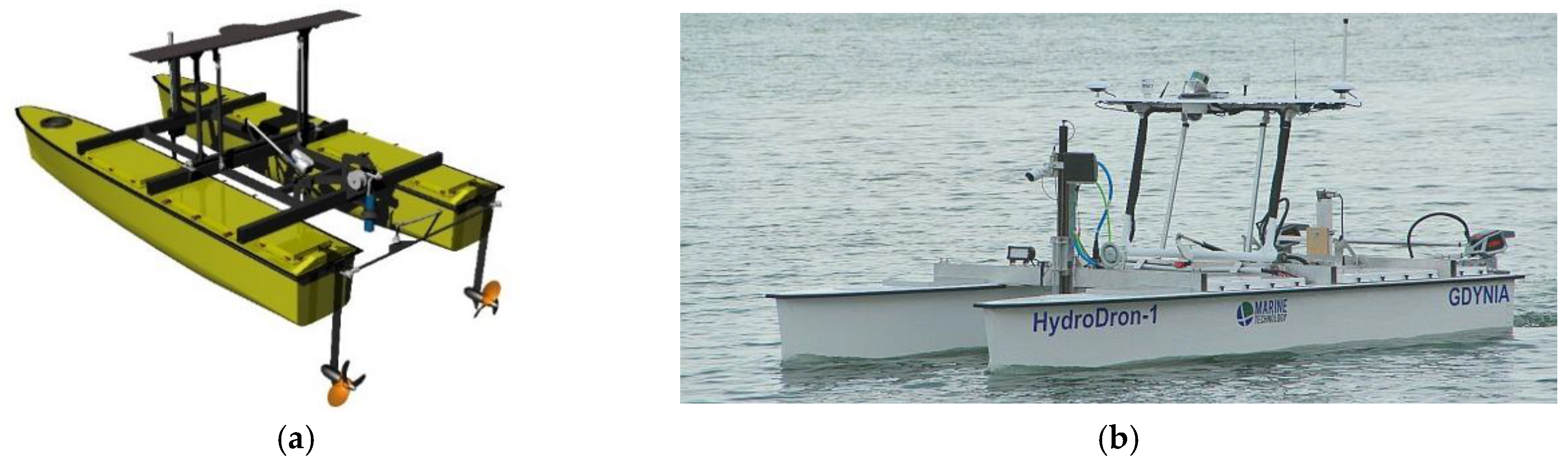
3. System Specification
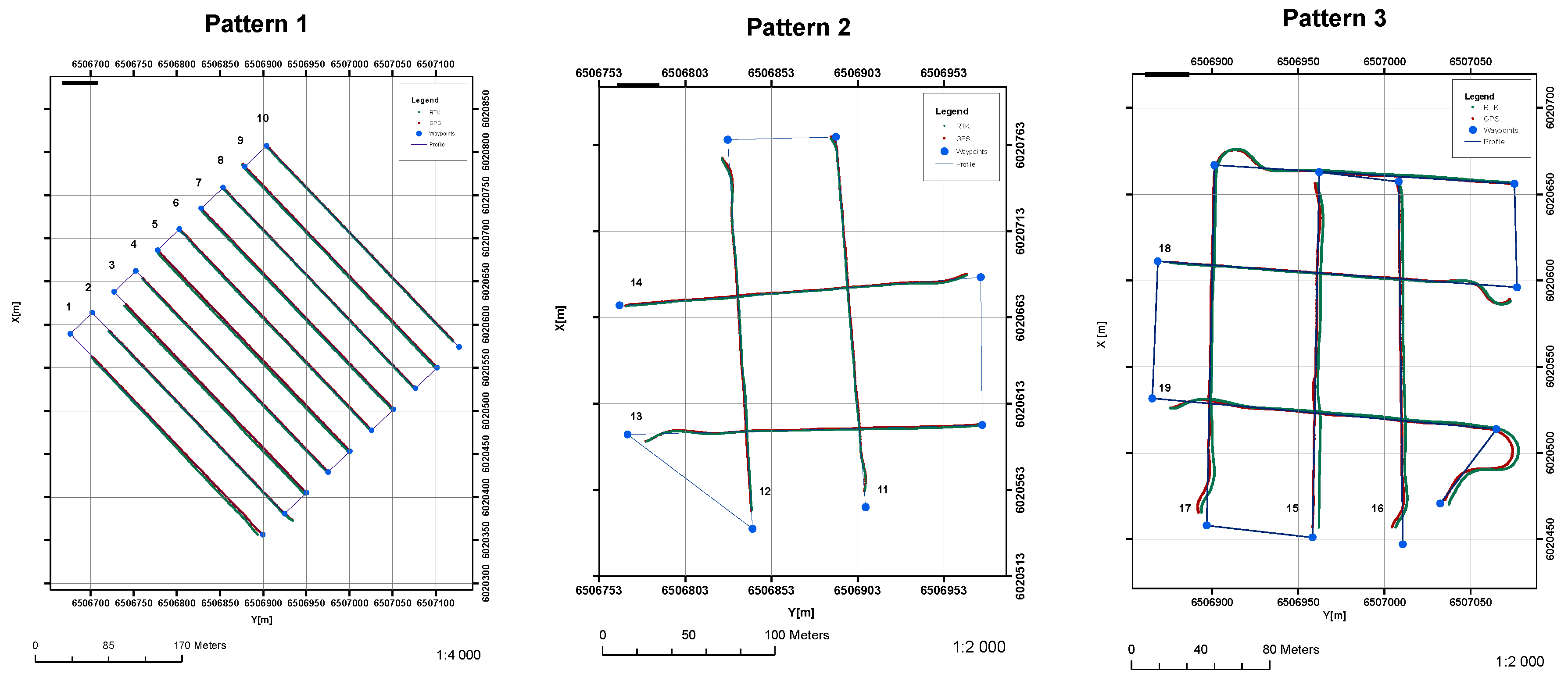
4. Experiments
4.1. Data Synchronization
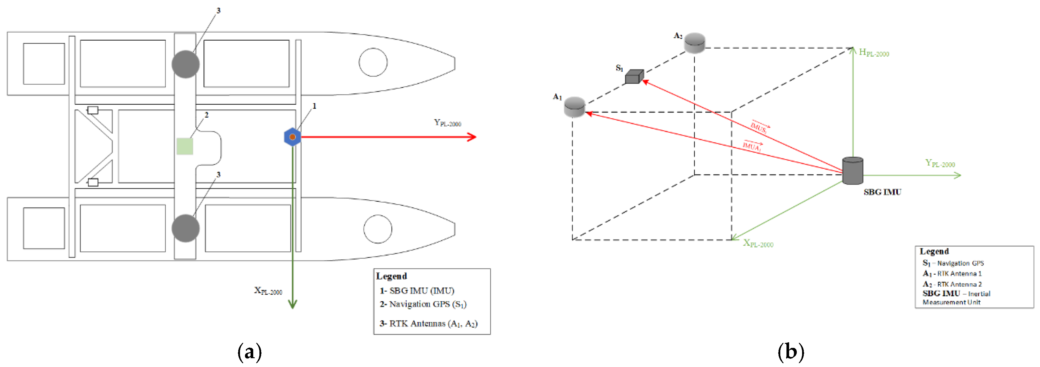
4.2. System Offsets
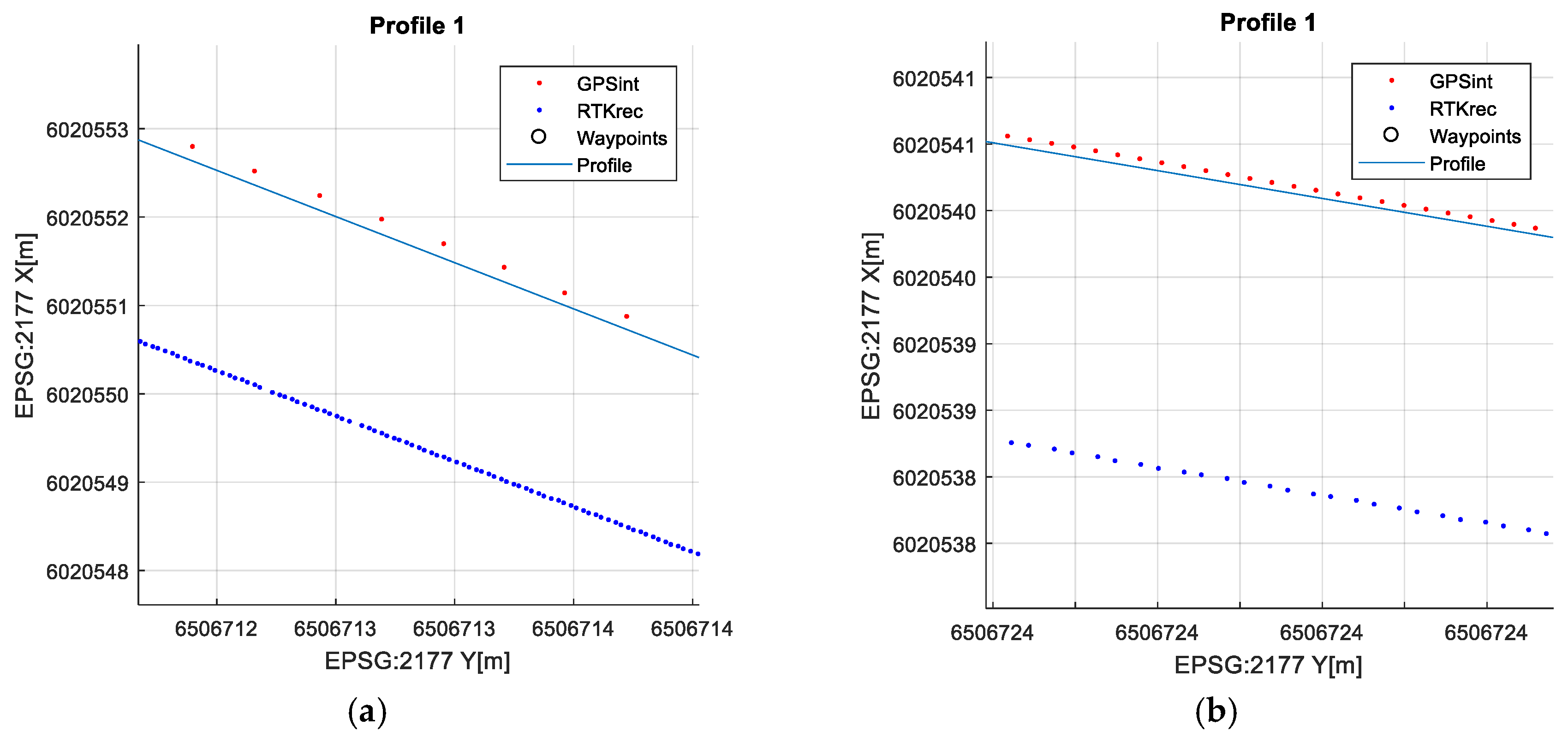
4.3. GPS Evaluation
4.4. Cross Track Error
5. Results
6. Discussion
7. Conclusions
Author Contributions
Funding
Conflicts of Interest
References
- Specht, M. Method of Evaluating the Positioning System Capability for Complying with the Minimum Accuracy Requirements for the International Hydrographic Organization Orders. Sensors 2019, 19, 3860. [Google Scholar] [CrossRef] [PubMed] [Green Version]
- Wang, N.; Er, M.J. Direct Adaptive Fuzzy Tracking Control of Marine Vehicles with Fully Unknown Parametric Dynamics and Uncertainties. IEEE Trans. Contr. Syst. Technol. 2016, 24, 1845–1852. [Google Scholar] [CrossRef]
- Wang, N.; Er, M.J.; Sun, J.; Liu, Y. Adaptive Robust Online Constructive Fuzzy Control of a Complex Surface Vehicle System. IEEE Trans. Cybern. 2016, 46, 1511–1523. [Google Scholar] [CrossRef] [PubMed]
- Liu, T.; Dong, Z.; Du, H.; Song, L.; Mao, Y. Path following control of the underactuated USV based on the improved line-of-sight guidance algorithm. Pol. Marit. Res. 2017, 24, 3–11. [Google Scholar] [CrossRef] [Green Version]
- Liao, Y.; Wan, L.; Zhuang, J. Back stepping dynamical sliding mode control method for the path following of the underactuated surface vessel. Procedia Eng. 2011, 15, 256–263. [Google Scholar] [CrossRef] [Green Version]
- Dong, Z.; Wan, L.; Li, Y.; Liu, T.; Zhang, G. Trajectory tracking control of underactuated USV based on modified backstepping approach. Int. J. Nav. Archit. Ocean Eng. 2015, 7, 817–832. [Google Scholar] [CrossRef] [Green Version]
- Fan, Y.; Mu, D.; Zhang, X.; Wang, G.; Guo, C. Course keeping control based on integrated nonlinear feedback for a USV with pod-like propulsion. J. Navig. 2018, 71, 878–898. [Google Scholar] [CrossRef]
- Huang, Q.; Li, T.; Li, Z.; Hang, Y.; Yang, S. Research on PID control technique for chaotic ship steering based on dynamic chaos particle swarm optimization algorithm. In Proceedings of the 10th World Congress on Intelligent Control and Automation, Beijing, China, 6–8 July 2012; pp. 1639–1643. [Google Scholar]
- Li, Y.; Yang, S.; Yu, Y.; Liu, M. Study on optimization and simulation of hydrofoil USV propulsion intelligent control based on chaos algorithm. In Proceedings of the 2017 2nd International Conference on Materials Science, Machinery and Energy Engineering (MSMEE 2017), Dalian, China, 13–14 May 2017. [Google Scholar] [CrossRef] [Green Version]
- Huang, Q.; Liu, X.; Li, T.; Wang, K.; Wang, S. On impulsive parametric perturbation control techniques for chaotic ship steering. In Proceedings of the Proceedings of 2014 IEEE Chinese Guidance, Navigation and Control Conference, Yantai, China, 8–10 August 2014; pp. 428–433. [Google Scholar]
- Wang, N.; Sun, J.; Er, M.J. Tracking-Error-Based Universal Adaptive Fuzzy Control for Output Tracking of Nonlinear Systems with Completely Unknown Dynamics. IEEE Trans. Fuzzy Syst. 2018, 26, 869–883. [Google Scholar] [CrossRef]
- Wang, N.; Su, S.; Yin, J.; Zheng, Z.; Er, M.J. Global Asymptotic Model-Free Trajectory-Independent Tracking Control of an Uncertain Marine Vehicle: An Adaptive Universe-Based Fuzzy Control Approach. IEEE Trans. Fuzzy Syst. 2018, 26, 1613–1625. [Google Scholar] [CrossRef]
- Patino, H.D.; Liu, D. Neural network-based model reference adaptive control system. IEEE Trans. Syst. Man Cybern. Part B (Cybern.) 2000, 30, 198–204. [Google Scholar] [CrossRef]
- Dai, S.-L.; Wang, C.; Luo, F. Identification and learning control of ocean surface ship using neural networks. IEEE Trans. Ind. Inform. 2012, 8, 801–810. [Google Scholar] [CrossRef]
- Zhang, Y.; Hearn, G.E.; Sen, P. A neural network approach to ship track-keeping control. IEEE J. Ocean. Eng. 1996, 21, 513–527. [Google Scholar] [CrossRef]
- Brown, M.; Harris, C.J. Neurofuzzy Adaptive Modelling and Control; Prentice Hall: Upper Saddle River, NJ, USA, 1994. [Google Scholar]
- Wang, N.; Joo Er, M. Self-Constructing Adaptive Robust Fuzzy Neural Tracking Control of Surface Vehicles with Uncertainties and Unknown Disturbances. IEEE Trans. Control Syst. Technol. 2015, 23, 991–1002. [Google Scholar] [CrossRef]
- Wang, N.; Sun, J.; Er, M.J.; Liu, Y. A Novel Extreme Learning Control Framework of Unmanned Surface Vehicles. IEEE Trans. Cybern. 2016, 46, 1106–1117. [Google Scholar] [CrossRef] [PubMed]
- Wang, N.; Karimi, H.R.; Li, H.; Su, S. Accurate Trajectory Tracking of Disturbed Surface Vehicles: A Finite-Time Control Approach. IEEE/ASME Trans. Mechatron. 2019, 24, 1064–1074. [Google Scholar] [CrossRef]
- Wang, N.; Qian, C.; Sun, J.; Liu, Y. Adaptive Robust Finite-Time Trajectory Tracking Control of Fully Actuated Marine Surface Vehicles. IEEE Trans. Control Syst. Technol. 2016, 24, 1454–1462. [Google Scholar] [CrossRef]
- Wang, N.; Pan, X. Path Following of Autonomous Underactuated Ships: A Translation–Rotation Cascade Control Approach. IEEE/ASME Trans. Mechatron. 2019, 24, 2583–2593. [Google Scholar] [CrossRef]
- Stateczny, A.; Burdziakowski, P. Universal autonomous control and management system for multipurpose unmanned surface vessel. Polish Marit. Res. 2019, 1, 30–39. [Google Scholar] [CrossRef] [Green Version]
- Stateczny, A.; Kazimierski, W.; Gronska-Sledz, D.; Motyl, W. The Empirical Application of Automotive 3D Radar Sensor for Target Detection for an Autonomous Surface Vehicle’s Navigation. Remote Sens. 2019, 11, 1156. [Google Scholar] [CrossRef] [Green Version]
- Park, S.; Deyst, J.; How, J. A new nonlinear guidance logic for trajectory tracking. AIAA Guid. Navig. Control Conf. Exhib. 2004. [Google Scholar] [CrossRef] [Green Version]
- Guo, W.; Wang, S.; Dun, W. The Design of a Control System for an Unmanned Surface Vehicle. Open Autom. Control Syst. J. 2015, 7, 50–156. [Google Scholar] [CrossRef] [Green Version]
- Moreno, D.; Chaos, D.; Aranda, J.; Muñoz, R.; Díaz, J.M.; Dormido-Canto, S. Application of an aeronautic control for ship path following. J. Marit. Res. 2009, 6, 71–82. [Google Scholar]
- Specht, C.; Specht, M.; Cywinski, P.; Skóra, M.; Marchel, Ł.; Szychowski, P. A New Method for Determining the Territorial Sea Baseline Using an Unmanned Hydrographic Surface Vessel. J. Coast. Res. 2019, 35, 925–936. [Google Scholar] [CrossRef]
- Specht, M.; Specht, C.; Lasota, H.; Cywinski, P. Assessment of the Steering Precision of a Hydrographic Unmanned Surface Vessel (USV) along Sounding Profiles Using a Low-Cost Multi-Global Navigation Satellite System (GNSS) Receiver Supported Autopilot. Sensors 2019, 19, 3939. [Google Scholar] [CrossRef] [Green Version]
- Seto, M.L.; Crawford, A. Autonomous shallow water bathymetric measurements for environmental assessment and safe navigation using USVs. In Proceedings of the OCEANS 2015-MTS/IEEE Washington, Washington, DC, USA, 19–22 October 2015. [Google Scholar]
- Alessandri, A.; Donnarumma, S.; Martelli, M.; Vignolo, S. Motion Control for Autonomous Navigation in Blue and Narrow Waters Using Switched Controllers. J. Mar. Sci. Eng. 2019, 7, 196. [Google Scholar] [CrossRef] [Green Version]
- Munoz-Banon, M.; del Pino, I.; Candelas, F.; Torres, F. Framework for Fast Experimental Testing of Autonomous Navigation Algorithms. Appl. Sci. Basel 2019, 9, 1997. [Google Scholar] [CrossRef] [Green Version]
- Kunicka, M.; Litwin, W. Energy Demand of Short-Range Inland Ferry with Series Hybrid Propulsion Depending on the Navigation Strategy. Energies 2019, 12, 3499. [Google Scholar] [CrossRef] [Green Version]
- Borkowski, P. Adaptive System for Steering a Ship along the Desired Route. Mathematics 2018, 6, 196. [Google Scholar] [CrossRef] [Green Version]
- Borkowski, P. Inference Engine in an Intelligent Ship Course-Keeping System. Comput. Intell. Neurosci. 2017. [Google Scholar] [CrossRef] [Green Version]
- Li, C.; Jiang, J.; Duan, F.; Liu, W.; Wang, X.; Bu, L.; Sun, Z.; Yang, G. Modeling and Experimental Testing of an Unmanned Surface Vehicle with Rudderless Double Thrusters. Sensors 2019, 19, 2051. [Google Scholar] [CrossRef] [Green Version]
- Zhan, W.; Xiao, C.; Wen, Y.; Zhou, C.; Yuan, H.; Xiu, S.; Zhang, Y.; Zou, X.; Liu, X.; Li, Q. Autonomous Visual Perception for Unmanned Surface Vehicle Navigation in an Unknown Environment. Sensors 2019, 19, 2216. [Google Scholar] [CrossRef] [PubMed] [Green Version]
- Lisowski, J. The sensitivity of state differential game vessel traffic model. Polish Marit. Res. 2016, 23, 14–18. [Google Scholar] [CrossRef] [Green Version]
- Dudojc, B.; Mindykowski, J. New Approach to Analysis of Selected Measurement and Monitoring Systems Solutions in Ship Technology. Sensors 2019, 19, 1775. [Google Scholar] [CrossRef] [PubMed] [Green Version]
- Li, J.; Du, J.; Sun, Y.; Lewis, F.L. Robust adaptive trajectory tracking control of underactuated autonomous underwater vehicles with prescribed performance. Int. J. Robust Nonlinear Control 2019, 29, 4629–4643. [Google Scholar] [CrossRef]
- Paliotta, C.; Lefeber, E.; Pettersen, K.; Pinto, J.; Costa, M.I.C.; de Sousa, J.T.D.B. Trajectory Tracking and Path Following for Underactuated Marine Vehicles. IEEE Trans. Control Syst. Technol. 2019, 27, 1423–1437. [Google Scholar] [CrossRef] [Green Version]
- GITHUB. Available online: https://github.com/ArduPilot/ardupilot/commit/a3c2851120f3572893bdf29ddc0ee24dac67cbe1 (accessed on 12 December 2019).
- Jang, T.; Han, S. Analysis for VTOL Flight Software of PX4. In Proceedings of the 2018 18th International Conference on Control, Automation and Systems (ICCAS), Daegwallyeong, South Korea, 17–20 October 2018; pp. 872–875. [Google Scholar]
- Siauw, T.; Bayen, A. An Introduction to MATLAB® Programming and Numerical Methods for Engineers; Academic Press: Cambridge, MA, USA, 2015. [Google Scholar] [CrossRef]
- Specht, C.; Dabrowski, P.S.; Pawelski, J.; Specht, M.; Szot, T. Comparative analysis of positioning accuracy of GNSS receivers of Samsung Galaxy smartphones in marine dynamic measurements. Adv. Space Res. 2019, 63, 3018–3028. [Google Scholar] [CrossRef]
- NovAtel Positioning Leadership. GPS Position Accuracy Measures. APN-029 Revision 1. 2003. Available online: https://www.novatel.com/assets/Documents/Bulletins/apn029.pdf (accessed on 12 December 2019).


| Specification | Data |
|---|---|
| Dimensions (L × W × H) | 4230 × 2080 × 1390 mm |
| Draft | 500 mm |
| Weight | 360 kg |
| Power supply | 48 V 200 Ah lithium iron phosphate battery (LiFePO4) (16 cells) for propulsion, 24 V lead-acid battery for electronics |
| Endurance | 12 h (cruise speed) |
| Motors | 2 × Torqeedo Cruise 4.0 |
| Remote control range | 40 km |
| Telemetry data range | 50 km |
| Payload data range | 6 km |
| Max speed | 14 knots |
| Parameter Name | Specification |
|---|---|
| Channels | 72 |
| Signal tracking: | GPS: L1C/A SBAS: L1C/A QZSS: L1C/A GLONASS: L1OF BeiDou: B1 Galileo: E1B/C2 |
| Horizontal position accuracy 1 | GPS and GLONAS: 2.5 m SBAS: 2.0 m |
| Velocity accuracy 2 | 0.05 m/s |
| True heading accuracy 2 | 0.3° |
| Operating limits | Altitude: 50,000 m Velocity: 500 m/s Acceleration: 4 g |
| Time to first fix | Cold start: <26 s Warm start: <1 s |
| Max output frequency | 5 Hz |
| Parameter Name | Specification |
|---|---|
| Channels | 220 |
| Signal tracking | GPS: L1 C/A, L2E, L2C, L5 GLONASS: L1 C/A, L2 C/A, L2 P, L3 CDMA Galileo: 1 BOC, E5A, E5B, E5AltBOC Beidou B1, B2 SBAS, QZSS L-Band OmniSTAR VBS, HP, XP |
| Horizontal position accuracy (1 sigma) | SBAS/DGPS: 0.5 m/0.25 m PPP: 10 cm RTK: 0.8 cm + 1 ppm |
| Velocity accuracy | 0.7 cm/s RMS |
| True heading accuracy | 0.09 ° at 2 m baseline 0.05 ° at 1 0m baseline |
| Operating limits | Altitude: 18,000 m Velocity: 515 m/s Acceleration: 11 g |
| Time to first fix | Cold start: <45 s Warm start: <30 s |
| Signal reacquisition | L1/L2/L5: <2.0 s |
| Max output frequency | 50 Hz |
| dy | dx | dH | |COGA1| | |COGS1| | Remarks | |
|---|---|---|---|---|---|---|
| GPS | −1.22 | 0.16 | 0.89 | 16.402 | For Equations (12) and (13) | |
| Origin | 0 | 0 | 0 | 15.186 | ||
| Antenna RTK 1 | −1.22 | −0.64 | 0.89 | In hydrographic system | ||
| Antenna RTK 2 | −1.22 | 0.96 | 0.89 | In hydrographic system |
| Coordinate Differences | Euclidean Distance | XTE |
|---|---|---|
 |  |  |
 |  |  |
 |  |  |
| Profile No. | σx | σy | DRMS | 2DRMS | CEP | R95 | Mean XTE |
|---|---|---|---|---|---|---|---|
| 1 | 0.4490 | 0.4788 | 0.6564 | 1.3129 | 0.5483 | 1.1405 | 0.1389 |
| 2 | 0.0599 | 0.0698 | 0.0920 | 0.1840 | 0.0768 | 0.1598 | 0.1080 |
| 3 | 0.1650 | 0.2108 | 0.2677 | 0.5354 | 0.2231 | 0.4640 | 0.0934 |
| 4 | 0.1029 | 0.0977 | 0.1419 | 0.2839 | 0.1182 | 0.2459 | 0.0578 |
| 5 | 0.1756 | 0.1975 | 0.2643 | 0.5286 | 0.2208 | 0.4592 | 0.0582 |
| 6 | 0.1698 | 0.1770 | 0.2453 | 0.4906 | 0.2048 | 0.4260 | 0.0881 |
| 7 | 0.1013 | 0.1447 | 0.1766 | 0.3533 | 0.1464 | 0.3046 | 0.0875 |
| 8 | 0.0857 | 0.0853 | 0.1209 | 0.2418 | 0.1009 | 0.2098 | 0.0911 |
| 9 | 0.0946 | 0.1044 | 0.1409 | 0.2817 | 0.1177 | 0.2448 | 0.0783 |
| 10 | 0.0783 | 0.0773 | 0.1101 | 0.2201 | 0.0918 | 0.1909 | 0.0750 |
| 11 | 0.2164 | 0.1547 | 0.2660 | 0.5320 | 0.2171 | 0.4516 | 0.2546 |
| 12 | 0.3149 | 0.0575 | 0.3201 | 0.6402 | 0.2120 | 0.4410 | 0.2433 |
| 13 | 0.1403 | 0.2244 | 0.2646 | 0.5293 | 0.2177 | 0.4528 | 0.3474 |
| 14 | 0.0591 | 0.1475 | 0.1589 | 0.3177 | 0.1245 | 0.2590 | 0.2315 |
| 15 | 0.2188 | 0.4595 | 0.5089 | 1.0179 | 0.4074 | 0.8475 | 0.3826 |
| 16 | 0.7284 | 0.2069 | 0.7572 | 1.5145 | 0.5362 | 1.1153 | 0.3218 |
| 17 | 0.5927 | 0.3553 | 0.6910 | 1.3821 | 0.5522 | 1.1486 | 1.5335 |
| 18 | 0.1795 | 0.3014 | 0.3508 | 0.7016 | 0.2874 | 0.5977 | 1.1249 |
| 19 | 0.1899 | 0.5650 | 0.5961 | 1.1922 | 0.4567 | 0.9499 | 0.4945 |
| σx | σy | DRMS | 2DRMS | CEP | R95 | Mean Unit XTE | |
|---|---|---|---|---|---|---|---|
| Mean | 0.2170 | 0.2166 | 0.3226 | 0.6452 | 0.2558 | 0.5321 | 0.3058 |
© 2020 by the authors. Licensee MDPI, Basel, Switzerland. This article is an open access article distributed under the terms and conditions of the Creative Commons Attribution (CC BY) license (http://creativecommons.org/licenses/by/4.0/).
Share and Cite
Stateczny, A.; Burdziakowski, P.; Najdecka, K.; Domagalska-Stateczna, B. Accuracy of Trajectory Tracking Based on Nonlinear Guidance Logic for Hydrographic Unmanned Surface Vessels. Sensors 2020, 20, 832. https://0-doi-org.brum.beds.ac.uk/10.3390/s20030832
Stateczny A, Burdziakowski P, Najdecka K, Domagalska-Stateczna B. Accuracy of Trajectory Tracking Based on Nonlinear Guidance Logic for Hydrographic Unmanned Surface Vessels. Sensors. 2020; 20(3):832. https://0-doi-org.brum.beds.ac.uk/10.3390/s20030832
Chicago/Turabian StyleStateczny, Andrzej, Pawel Burdziakowski, Klaudia Najdecka, and Beata Domagalska-Stateczna. 2020. "Accuracy of Trajectory Tracking Based on Nonlinear Guidance Logic for Hydrographic Unmanned Surface Vessels" Sensors 20, no. 3: 832. https://0-doi-org.brum.beds.ac.uk/10.3390/s20030832