Estimating Occupancy Levels in Enclosed Spaces Using Environmental Variables: A Fitness Gym and Living Room as Evaluation Scenarios

 , , , and
Abstract
:1. Introduction
- Two datasets built with real-world information: one dataset collected from a fitness gym and another gathered from the living room in a house inhabited by seven people.
- The evaluation of three Machine Learning algorithms: Support Vector Machine (SVM), k-Nearest Neighbor (kNN), and Decision Trees (DT), to estimate 3-4 occupancy levels with different temporal resolutions using the built datasets and only the temperature, humidity, and pressure values.
2. Related Work
3. Estimating Occupancy Levels in Enclosed Spaces Using Environmental Variables
3.1. Methodology
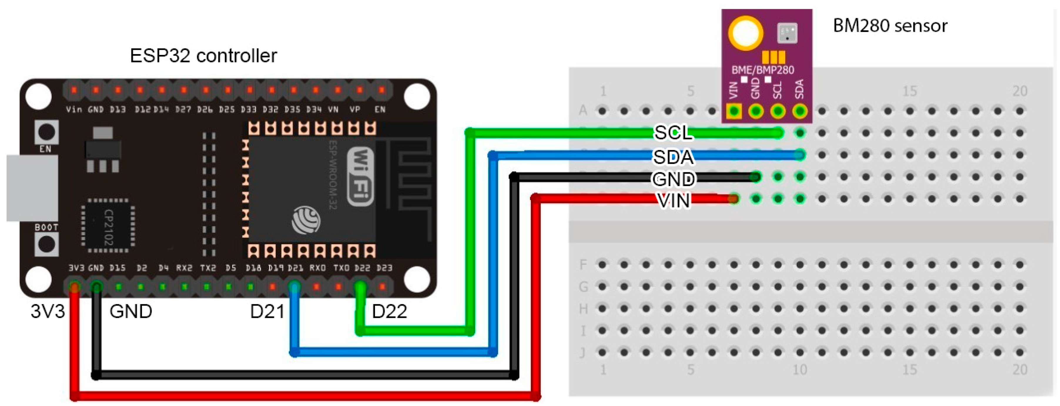
- Definition of the collection sensors. The sensors used to collect the data are of utmost importance since the quality of the data available for further analysis and experimentation will depend on them. For the specific case of this research, sensors capable of collecting temperature, humidity, and pressure values with a resolution of 1 s are required in order to obtain a high-resolution dataset. This feature is key as one objective of this research is to explore the effects of data resolution on the prediction of occupation.
- Data collection. Two different locations will be selected for the data collection. This will allow obtaining independent datasets to contrast and enrich the results obtained from the experimentation.
- Data preprocessing. A curation of the data will be performed to remove missing values, analyze and update/remove sensor reading errors, standardize collected data, and integrate the labels corresponding to the occupancy levels for each record. All this processing will improve the quality of the collected data for further experimentation and publication.
- Data exploration. A visual exploration of the data will be carried out to find patterns and characteristics that could help in the interpretation of the results produced by the predictive models.
- Selection of prediction models. Three Machine Learning models widely used in the detection and estimation of occupancy levels will be selected through a review of the literature.
- Design of experimentation and evaluation scenarios. Experimentation scenarios will be designed to find an optimal subset of attributes as well as the optimal resolution of the dataset. In the same way, assessment scenarios will be proposed using the selected evaluation metric, which will allow comparing the results to determine the best estimation algorithm.
3.2. Definition of the Collection Sensors
3.3. Data Collection
3.3.1. Fitness Gym
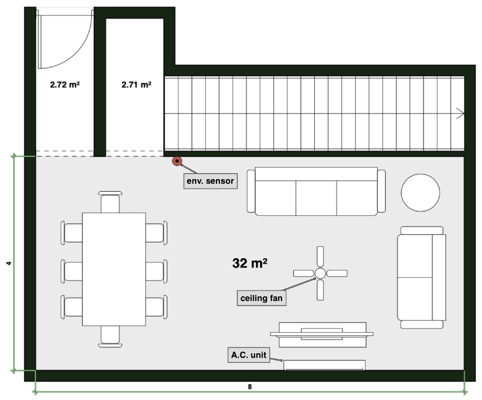
3.3.2. Living Room
3.4. Data Preprocessing
3.4.1. Establishing the Occupancy Levels
3.4.2. Generating of Datasets with Different Resolutions
3.4.3. Partitioning and Balancing
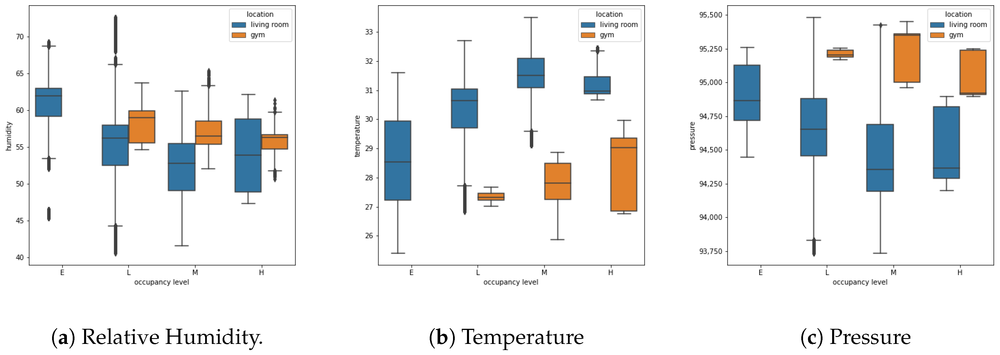
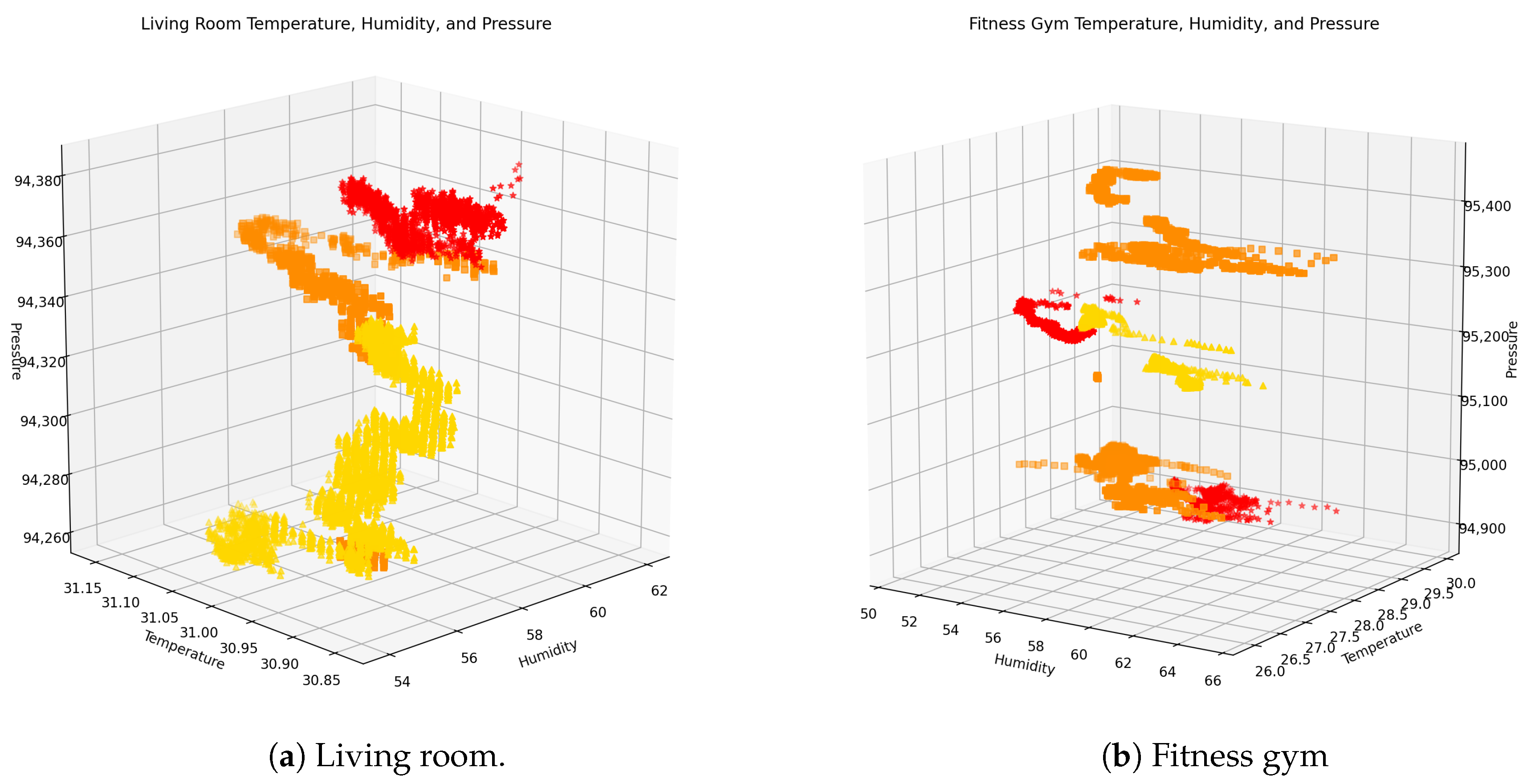
3.5. Data Exploration
3.6. Selection of Prediction Models
- k-Nearest Neighbor (kNN): This is a classifier based on the concept of similarity. It finds the k neighbors most “similar” to the instance to be classified, and assign the statistical mode as the class of the new instance. Although there are several similarity measures, such as Manhattan, Minkowski, and Chebyshev, Euclidean distance was selected for this work because of its ease of being generalized in domains of n features [28]. Another important parameter is k, the number of neighbors used to classify each point. It is important to choose the value of k carefully since a low value increases the model bias but a value too high produce overfitting and an increment in the computational cost.
- Support Vector Machine (SVM): This algorithm can be used for classification and regression. It works by performing a projection of the data points to a higher dimension, where they can be separated using a line or a hyperplane [29]. The points that lie exactly at the limit of the decision surface are called Support Vectors. For the systemic search of the optimal hyperplane, a kernel function is used. Examples of some kernels are (but are not limited to): linear, polynomial, and radial base function (RBF). Besides the kernel, other important parameters of the model are the regularization parameter C and Gamma, which control the tolerance to classification errors and how large the area of influence of the decision boundary is (for non-linear kernels), respectively.
- Decision Trees (DT): This classifier works by creating a tree based on the features. Each non-leaf node of the tree represents a partitioning rule of the dataset using some attribute. The tree is recursively created by calculating the importance of each feature after a split. An important benefit of DT is that the result can be easily interpreted, i.e., to understand why a specific point was assigned to a class, just read the rule at each node. Among the parameters to optimize the model are the maximum depth, the minimum number of instances to make a separation, and the criteria to determine the importance of each attribute [28].
3.7. Design of Experimentation and Evaluation Scenarios
- Feature Selection: To find the optimal subset of features, two feature selection techniques were implemented: (i) recursive feature elimination (RFE), and (ii) k-best with ANOVA F-value as score function. Chi-square was discarded as a score function due to the data contains negative values. This experiment was executed on the averaged 10-s datasets. This is because they are the highest resolution datasets that contain the extra attributes (kurtosis and standard deviation). For each scenario, the prediction was made using the following datasets:
- -
- FULL: 10 s averaged dataset with nine attributes (including kurtosis and standard deviation for humidity, pressure, and temperature).
- -
- RFE: 10 s averaged dataset with five best features selected by the RFE technique.
- -
- KBEST: 10 s averaged dataset with five best features selected by the k-best technique.
- -
- MIN: 10 s averaged dataset with three features (humidity, pressure, and temperature).
- Resolution Selection: Predictions using the distinct resolution datasets were performed: 10 s, 30 s, 1 min, and 5 min. Additionally, predictions were also made using the corresponding averaged datasets to contrast the performance of the models using a single sample against the averages.
Evaluation Metrics
4. Results and Discussion
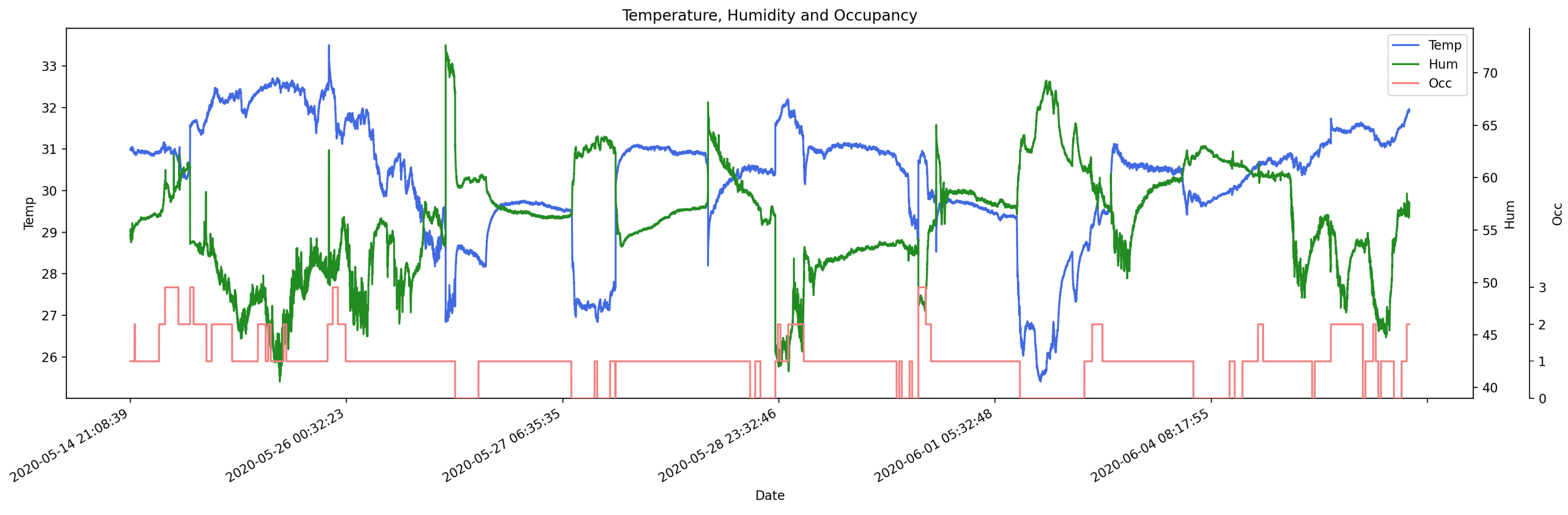
4.1. Visual Exploration
4.2. Experimentation Setup
4.3. Fitness Gym
4.4. Living Room
4.5. Comparison with Other Approaches
5. Conclusions and Further Work
Supplementary Materials
Author Contributions
Funding
Acknowledgments
Conflicts of Interest
Abbreviations
| AC | Air Conditioner |
| ADASYN | Adaptive Synthetic |
| BLE | Bluetooth Low Energy |
| CART | Classification and Regression Trees |
| DT | Decision Trees |
| EC | Edge Computing |
| ELM | Extreme Learning Machine |
| FNN | Feedforward Neural Network |
| GB | Gradient Boost |
| HMM | Hidden Markov Model |
| HVAC | Heating, Ventilation, and Air Conditioners |
| IEA | International Energy Agency |
| IoT | Internet of Things |
| kNN | K-Nearest Neighbor |
| LDA | Linear Discriminant Analysis |
| LR | Logistic Regression |
| LSTM | Long Short-Term Memory |
| MLP | Multilayer Perceptron |
| MM | Markov Model |
| PIR | Passive Infrared |
| RF | Random Forest |
| RFE | Recursive Feature Elimination |
| RFID | Radio Frequency Identification |
| SRAM | Static Random Access Memory |
| SVM | Support Vector Machine |
| UCI | University of California, Irvine |
| VOC | Volatile Organic Compound |
| WiFi | Wireless Fidelity |
References
- Yuan, Y.; Li, X.; Liu, Z.; Guan, X. Occupancy estimation in buildings based on infrared array sensors detection. IEEE Sens. J. 2019, 20, 1043–1053. [Google Scholar] [CrossRef]
- Oldewurtel, F.; Sturzenegger, D.; Morari, M. Importance of occupancy information for building climate control. Appl. Energy 2013, 101, 521–532. [Google Scholar] [CrossRef]
- Yan, D.; Hong, T.; Dong, B.; Mahdavi, A.; D’Oca, S.; Gaetani, I.; Feng, X. IEA EBC Annex 66: Definition and simulation of occupant behavior in buildings. Energy Build. 2017, 156, 258–270. [Google Scholar] [CrossRef] [Green Version]
- O’Brien, W.; Wagner, A.; Schweiker, M.; Mahdavi, A.; Day, J.; Kjærgaard, M.B.; Carlucci, S.; Dong, B.; Tahmasebi, F.; Yan, D.; et al. Introducing IEA EBC Annex 79: Key challenges and opportunities in the field of occupant-centric building design and operation. Build. Environ. 2020, 106738. [Google Scholar] [CrossRef]
- Kumar, S.; Singh, J.; Singh, O. Ensemble-based extreme learning machine model for occupancy detection with ambient attributes. Int. J. Syst. Assur. Eng. Manag. 2020, 11, 173–183. [Google Scholar] [CrossRef]
- Hong, T.; Yan, D.; D’Oca, S.; Chen, C.F. Ten questions concerning occupant behavior in buildings: The big picture. Build. Environ. 2017, 114, 518–530. [Google Scholar] [CrossRef] [Green Version]
- Huchuk, B.; Sanner, S.; O’Brien, W. Comparison of machine learning models for occupancy prediction in residential buildings using connected thermostat data. Build. Environ. 2019, 160, 106177. [Google Scholar] [CrossRef]
- Viani, F.; Polo, A.; Robol, F.; Oliveri, G.; Rocca, P.; Massa, A. Crowd detection and occupancy estimation through indirect environmental measurements. In Proceedings of the 8th European Conference on Antennas and Propagation (EuCAP 2014), Hague, The Netherlands, 6–11 April 2014. [Google Scholar] [CrossRef]
- Fiebig, F.; Kochanneck, S.; Mauser, I.; Schmeck, H. Detecting occupancy in smart buildings by data fusion from low-cost sensors. In Proceedings of the 8th International Conference on Future Energy Systems, Hong Kong, China, 16–19 May 2017; pp. 259–261. [Google Scholar] [CrossRef]
- Zemouri, S.; Gkoufas, Y.; Murphy, J. A Machine Learning Approach to Indoor Occupancy Detection Using Non-Intrusive Environmental Sensor Data. In Proceedings of the 3rd International Conference on Big Data and Internet of Things (BDIOT 2019), Melbourn, VIC, Australia, 22–24 August 2019; pp. 70–74. [Google Scholar] [CrossRef]
- Zhou, Y.; Chen, J.; Yu, Z.J.; Li, J.; Huang, G.; Haghighat, F.; Zhang, G. A novel model based on multi-grained cascade forests with wavelet denoising for indoor occupancy estimation. Build. Environ. 2020, 167, 106461. [Google Scholar] [CrossRef]
- Adeogun, R.; Rodriguez, I.; Razzaghpour, M.; Berardinelli, G.; Christensen, P.H.; Mogensen, P.E. Indoor occupancy detection and estimation using machine learning and measurements from an IoT LoRa-based monitoring system. In Proceedings of the Global IoT Summit (GIoTS 2019), Aarhus, Denmark, 17–21 June 2019; pp. 1–5. [Google Scholar] [CrossRef] [Green Version]
- Parise, A.; Manso-Callejo, M.A.; Cao, H.; Mendonca, M.; Kohli, H.; Wachowicz, M. Indoor Occupancy Prediction using an IoT Platform. In Proceedings of the 2019 6th International Conference on Internet of Things: Systems, Management and Security (IOTSMS 2019), Granada, Spain, 22–25 October 2019; pp. 26–31. [Google Scholar] [CrossRef]
- Makonin, S. ODDs: Occupancy Detection Dataset. 2015. Available online: https://dataverse.harvard.edu/dataset.xhtml?persistentId=doi:10.7910/DVN/2K9FFE (accessed on 25 May 2020).
- Willocx, M. Occupancy Detection in a Student Room. 2019. Available online: https://dataverse.harvard.edu/dataset.xhtml?persistentId=doi:10.7910/DVN/BIIFAJ (accessed on 25 May 2020).
- Hobson, B.W.; Lowcay, D.; Gunay, H.B.; Ashouri, A.; Newsham, G.R. Opportunistic occupancy-count estimation using sensor fusion: A case study. Build. Environ. 2019, 159, 106154. [Google Scholar] [CrossRef]
- Mashmn—Occupancy Dataset. Available online: https://github.com/mashmn/OccupancyDetection (accessed on 25 May 2020).
- Candanedo, L.M.; Feldheim, V. Accurate occupancy detection of an office room from light, temperature, humidity and CO2 measurements using statistical learning models. Energy Build. 2016, 112, 28–39. [Google Scholar] [CrossRef]
- Ecobee—Donate Your Data. Available online: https://www.ecobee.com/donate-your-data/ (accessed on 25 May 2020).
- Calì, D.; Matthes, P.; Huchtemann, K.; Streblow, R.; Müller, D. CO2 based occupancy detection algorithm: Experimental analysis and validation for office and residential buildings. Build. Environ. 2015, 86, 39–49. [Google Scholar] [CrossRef]
- Chitu, C.; Stamatescu, G.; Stamatescu, I.; Sgârciu, V. Assessment of Occupancy Estimators for Smart Buildings. In Proceedings of the 2019 10th IEEE International Conference on Intelligent Data Acquisition and Advanced Computing Systems: Technology and Applications (IDAACS), Metz, France, 18–21 September 2019; Volume 1, pp. 228–233. [Google Scholar]
- Jiang, C.; Chen, Z.; Su, R.; Masood, M.K.; Soh, Y.C. Bayesian filtering for building occupancy estimation from carbon dioxide concentration. Energy Build. 2020, 206, 109566. [Google Scholar] [CrossRef]
- Arendt, K.; Johansen, A.; Jørgensen, B.N.; Kjærgaard, M.B.; Mattera, C.G.; Sangogboye, F.C.; Schwee, J.H.; Veje, C.T. Room-Level Occupant Counts, Airflow and CO2 Data from an Office Building. In Proceedings of the First Workshop on Data Acquisition to Analysis (DATA ’18), Shenzhen, China, 4 November 2018; Association for Computing Machinery: New York, NY, USA, 2018; pp. 13–14. [Google Scholar] [CrossRef]
- BME280 Bosh Datasheet. Available online: https://www.bosch-sensortec.com/products/environmental-sensors/humidity-sensors-bme280/ (accessed on 25 May 2020).
- ESP32 Expressiff Datasheet. Available online: https://www.espressif.com/en/products/socs/esp32/overview (accessed on 25 May 2020).
- Mansour, E.; Vishinkin, R.; Rihet, S.; Saliba, W.; Fish, F.; Sarfati, P.; Haick, H. Measurement of temperature and relative humidity in exhaled breath. Sens. Actuators B 2020, 304, 127371. [Google Scholar] [CrossRef]
- He, H.; Bai, Y.; Garcia, E.A.; Li, S. ADASYN: Adaptive synthetic sampling approach for imbalanced learning. In Proceedings of the 2008 IEEE International Joint Conference on Neural Networks (IEEE World Congress on Computational Intelligence), Hong Kong, China, 1–8 June 2008; pp. 1322–1328. [Google Scholar]
- Kubat, M. An Introduction to Machine Learning; Springer: Berlin/Heidelberg, Germany, 2017. [Google Scholar]
- Cortes, C.; Vapnik, V. Support-vector networks. Mach. Learn. 1995, 20, 273–297. [Google Scholar] [CrossRef]
- Scikit-Learn. Available online: https://scikit-learn.org/stable/index.html (accessed on 25 May 2020).
- Szczurek, A.; Maciejewska, M.; Pietrucha, T. Occupancy Detection using Gas Sensors. In Proceedings of the 6th International Conference on Sensor Networks (SENSORNETS 2017), Porto, Portugal, 19–21 February 2017; pp. 99–107. [Google Scholar]
- Pedersen, T.H.; Nielsen, K.U.; Petersen, S. Method for room occupancy detection based on trajectory of indoor climate sensor data. Build. Environ. 2017, 115, 147–156. [Google Scholar] [CrossRef]
- Zemouri, S.; Magoni, D.; Zemouri, A.; Gkoufas, Y.; Katrinis, K.; Murphy, J. An edge computing approach to explore indoor environmental sensor data for occupancy measurement in office spaces. In Proceedings of the 2018 IEEE International Smart Cities Conference (ISC2). IEEE, Kansas City, MO, USA, 16–19 September 2018; pp. 1–8. [Google Scholar]
- CONAGUA Weather Information by Entity. Available online: https://smn.conagua.gob.mx/es/informacion-climatologica-por-estado?estado=nl (accessed on 25 May 2020).


| Author | Year | Variables | Algo. | OR | SR | TR | BR | GT | Demo Scale | Dataset |
|---|---|---|---|---|---|---|---|---|---|---|
| Viani et al. [8] | 2014 | temp., hum., CO | SVM | 2 | 3 | N/A | 0.82 acc. | N/A | 29 IoT nodes | own |
| Cali et al. [20] | 2015 | CO Prof., CO, windows, doors | Mass balance | 2 | 3 | N/A | 0.79 custom. | man. | 8 d., 5 rooms | own |
| Fiebig et al. [9] | 2017 | VOC, Network, Bt. K.F., calendar | MLP, kNN, DT, RF | 1 | 1 | N/A | 0.75 F1 | man. | 52 d., 2 bedroom apt. | own |
| Parise et al. [13] | 2019 | temp., hum., CO, PIR | SVM | 1 | 3 | 10 s | 0.96 F1 | N/A | 2 weeks, 1 room | own |
| Adeogun et al. [12] | 2019 | press, hum., CO, PIR, windows, doors | FNN | 2 | 3 | 5 min | 0.91 acc. | man. | 6 weeks, 2 off., 4 pers. | own |
| Zemouri et al. [10] | 2019 | temp., hum. | LR, LDA, kNN, CART, NB, SVM, GB | 1 | 3 | 5 min | 0.83 acc. | video | 37 d., 1 off., 3 pers. | own |
| Huchuck et al. [7] | 2019 | temp., hum., o. temp., PIR, others | LR, MM, HMM, RF, LSTM | 1 | 3 | 30 min | 0.75 acc. | No | 1 year, 100 tstat. | DYP [19] |
| Chitu et al. [21] | 2019 | CO, Air Flow | RF, ELM | 2 | 3 | 1 min | 69.17 acc. | algo. | 15 d., 4 rooms | USD-OD [23] |
| Jiang et al. [22] | 2020 | CO | Bayessian Filtering with ELM and IMM | 2 | 3 | 15 min | 0.77 acc. | video | 30 d., 1 off., 28 pers. | own |
| Kumar et al. [5] | 2020 | temp., hum., hum. ratio, CO, light | ELM | 1 | 3 | 1 min | 0.99 acc. | photos | building office | UCI [18] |
| Zhou et al. [11] | 2020 | CO | gcForest | 2 | 2 | 1 min | 0.82 acc. | video | 20 d., 1 lab., 4 pers. | own |
| Yuan et al. [1] | 2020 | IR array sensor, temp. | IHMM | 2 | 3 | N/A | 0.81 acc. | video | 6 IoT nodes, 1 lab. | own |
| Dataset | Before | After | ||||||
|---|---|---|---|---|---|---|---|---|
| Class | Empty | Low | Medium | High | Empty | Low | Medium | High |
| Living room 10 s | 4098 | 16,325 | 2830 | 547 | 16,353 | 16,325 | 16,330 | 16,329 |
| Living room 30 s | 1345 | 5450 | 956 | 188 | 5445 | 5450 | 5436 | 5452 |
| Living room 1 min | 673 | 2730 | 480 | 92 | 2720 | 2730 | 2720 | 2732 |
| Living room 5 min | 136 | 553 | 96 | 19 | 556 | 553 | 555 | 554 |
| Gym 10 s | N/A | 202 | 430 | 189 | N/A | 430 | 430 | 430 |
| Gym 30 s | N/A | 149 | 149 | 59 | N/A | 149 | 149 | 150 |
| Gym 1 min | N/A | 33 | 77 | 34 | N/A | 77 | 77 | 77 |
| Gym 5 min | N/A | 21 | 9 | 5 | N/A | 21 | 21 | 21 |
| Location | Dataset | DT | kNN | SVM | |||
|---|---|---|---|---|---|---|---|
| Criterion | Max Depth | Algorithm | Neighbors | c | Gamma | ||
| Feature Selection Fitness Gym | FULL | entropy | 10 | ball_tree | 1 | 10 | 1 |
| RFE | entropy | 6 | ball_tree | 1 | 1 | 1 | |
| KBEST | entropy | 10 | ball_tree | 1 | 1 | 1 | |
| MIN | entropy | 8 | ball_tree | 1 | 1 | 1 | |
| Feature Selection Living Room | FULL | gini | 12 | ball_tree | 1 | N/A | N/A |
| RFE | gini | 12 | ball_tree | 1 | N/A | N/A | |
| KBEST | gini | 12 | ball_tree | 1 | N/A | N/A | |
| MIN | gini | 12 | ball_tree | 1 | N/A | N/A | |
| Resolution Selection Fitness Gym | 10 s | entropy | 8 | ball_tree | 1 | 1 | 1 |
| 10 avg. | entropy | 10 | ball_tree | 1 | 1 | 1 | |
| 30 s | entropy | 16 | ball_tree | 1 | 1 | 1 | |
| 30 avg. | entropy | 14 | ball_tree | 1 | 1 | 1 | |
| 1 min | entropy | 14 | ball_tree | 1 | 1 | 1 | |
| 1 avg. | gini | 16 | ball_tree | 1 | 1 | 1 | |
| Resolution Selection Living Room | 10 s | entropy | 22 | ball_tree | 1 | 100 | 10 |
| 10 avg. | entropy | 24 | ball_tree | 1 | 100 | 10 | |
| 30 s | entropy | 22 | ball_tree | 1 | 100 | 10 | |
| 30 avg. | entropy | 22 | ball_tree | 1 | 100 | 10 | |
| 1 min | entropy | 20 | ball_tree | 1 | 100 | 10 | |
| 1 avg. | gini | 20 | ball_tree | 1 | 100 | 10 | |
| 5 min | entropy | 18 | ball_tree | 1 | 100 | 10 | |
| 5 avg. | entropy | 12 | ball_tree | 1 | 100 | 10 | |
| Humidity | Temperature | Pressure | |||||||
|---|---|---|---|---|---|---|---|---|---|
| Mean | Kurt | Std | Mean | Kurt | Std | Mean | Kurt | Std | |
| FULL | X | X | X | X | X | X | X | X | X |
| RFE | X | X | X | X | X | ||||
| KBEST | X | X | X | X | X | ||||
| MIN | X | X | X | ||||||
| Living Room | Fitness Gym | |||||||||
|---|---|---|---|---|---|---|---|---|---|---|
| FULL | RFE | KBEST | MIN | Mean | FULL | RFE | KBEST | MIN | Mean | |
| SVM | NA | NA | NA | NA | 0.9512 | 1.0 | 0.9951 | 1.0 | 0.9866 | |
| kNN | 0.7868 | 0.9231 | 0.9172 | 0.9848 | 0.9030 | 0.9512 | 1.0 | 0.9853 | 1.0 | 0.9841 |
| DT | 0.9441 | 0.9562 | 0.9586 | 0.9663 | 0.9563 | 0.9951 | 0.9951 | 0.9902 | 1.0 | 0.9951 |
| Mean | 0.8655 | 0.9397 | 0.9379 | 0.9756 | 0.9658 | 0.9984 | 0.9902 | 1.0 | ||
| 1 Sample | Averaged | |||||||
|---|---|---|---|---|---|---|---|---|
| 10 s | 30 s | 1 min | Mean | 10 s | 30 s | 1 min | Mean | |
| SVM | 0.9951 | 1.0 | 1.0 | 0.9984 | 1.0 | 0.9857 | 1.0 | 0.9952 |
| kNN | 0.9951 | 1.0 | 1.0 | 0.9984 | 1.0 | 1.0 | 1.0 | 1.0 |
| DT | 1.0 | 1.0 | 0.9722 | 0.9907 | 0.9902 | 1.0 | 1.0 | 0.9967 |
| Mean | 0.9967 | 1.0 | 0.9907 | 0.9967 | 0.9952 | 1.0 | ||
| Humidity | Temperature | Pressure | |||||||
|---|---|---|---|---|---|---|---|---|---|
| Mean | Kurt | Std | Mean | Kurt | Std | Mean | Kurt | Std | |
| FULL | X | X | X | X | X | X | X | X | X |
| RFE | X | X | X | X | X | ||||
| KBEST | X | X | X | X | X | ||||
| MIN | X | X | X | ||||||
| 1 Sample | Averaged | |||||||||
|---|---|---|---|---|---|---|---|---|---|---|
| 10 s | 30 s | 1 min | 5 min | Mean | 10 s | 30 s | 1 min | 5 min | Mean | |
| SVM | 0.9716 | 0.9652 | 0.9517 | 0.9054 | 0.9485 | 0.9756 | 0.9657 | 0.9657 | 0.8955 | 0.9506 |
| kNN | 0.9848 | 0.9753 | 0.9577 | 0.9104 | 0.9571 | 0.9882 | 0.9768 | 0.9607 | 0.9452 | 0.9677 |
| DT | 0.9825 | 0.9712 | 0.9436 | 0.8358 | 0.9333 | 0.9831 | 0.9743 | 0.9476 | 0.9054 | 0.9526 |
| Mean | 0.9796 | 0.9706 | 0.9510 | 0.8839 | 0.9823 | 0.9723 | 0.9580 | 0.9154 | ||
| Viani et al. [8] | Adeogun et al. [12] | Chitu et al. [21] | Jiang et al. [22] | Zhou et al. [11] | Fitness Gym | Living Room | |
|---|---|---|---|---|---|---|---|
| Accuracy | 0.82 | 0.91 | 0.69 | 0.77 | 0.82 | 1.0 | 0.98 |
| Variables | temp. hum. CO | temp. pre. hum. 7 more | CO air flow | CO | CO | temp. hum. pre. | temp. hum pre. |
Publisher’s Note: MDPI stays neutral with regard to jurisdictional claims in published maps and institutional affiliations. |
© 2020 by the authors. Licensee MDPI, Basel, Switzerland. This article is an open access article distributed under the terms and conditions of the Creative Commons Attribution (CC BY) license (http://creativecommons.org/licenses/by/4.0/).
Share and Cite
Vela, A.; Alvarado-Uribe, J.; Davila, M.; Hernandez-Gress, N.; Ceballos, H.G. Estimating Occupancy Levels in Enclosed Spaces Using Environmental Variables: A Fitness Gym and Living Room as Evaluation Scenarios. Sensors 2020, 20, 6579. https://0-doi-org.brum.beds.ac.uk/10.3390/s20226579
Vela A, Alvarado-Uribe J, Davila M, Hernandez-Gress N, Ceballos HG. Estimating Occupancy Levels in Enclosed Spaces Using Environmental Variables: A Fitness Gym and Living Room as Evaluation Scenarios. Sensors. 2020; 20(22):6579. https://0-doi-org.brum.beds.ac.uk/10.3390/s20226579
Chicago/Turabian StyleVela, Andree, Joanna Alvarado-Uribe, Manuel Davila, Neil Hernandez-Gress, and Hector G. Ceballos. 2020. "Estimating Occupancy Levels in Enclosed Spaces Using Environmental Variables: A Fitness Gym and Living Room as Evaluation Scenarios" Sensors 20, no. 22: 6579. https://0-doi-org.brum.beds.ac.uk/10.3390/s20226579