Article

Sensitivity of the Enhanced Vegetation Index (EVI) and Normalized Difference Vegetation Index (NDVI) to Topographic Effects: A Case Study in High-density Cypress Forest

1
Graduate School of Life and Environmental Sciences, University of Tsukuba, 1-1-1 Tennoudai, Tsukuba, Ibaraki, 305-8572, Japan
2
Key Laboratory of Environment Change and Natural Disaster, Ministry of Education of China, College of Resource Science and Technology, Beijing Normal University, Beijing 100875, China
*
Author to whom correspondence should be addressed.
Sensors 2007, 7(11), 2636-2651; https://0-doi-org.brum.beds.ac.uk/10.3390/s7112636
Submission received: 2 August 2007 / Accepted: 30 October 2007 / Published: 5 November 2007
(This article belongs to the Special Issue Remote Sensing of Natural Resources and the Environment)

Abstract

:
Vegetation indices play an important role in monitoring variations in vegetation. The Enhanced Vegetation Index (EVI) proposed by the MODIS Land Discipline Group and the Normalized Difference Vegetation Index (NDVI) are both global-based vegetation indices aimed at providing consistent spatial and temporal information regarding global vegetation. However, many environmental factors such as atmospheric conditions and soil background may produce errors in these indices. The topographic effect is another very important factor, especially when the indices are used in areas of rough terrain. In this paper, we theoretically analyzed differences in the topographic effect on the EVI and the NDVI based on a non-Lambertian model and two airborne-based images acquired from a mountainous area covered by high-density Japanese cypress plantation were used as a case study. The results indicate that the soil adjustment factor “L” in the EVI makes it more sensitive to topographic conditions than is the NDVI. Based on these results, we strongly recommend that the topographic effect should be removed in the reflectance data before the EVI was calculated—as well as from other vegetation indices that similarly include a term without a band ratio format (e.g., the PVI and SAVI)—when these indices are used in the area of rough terrain, where the topographic effect on the vegetation indices having only a band ratio format (e.g., the NDVI) can usually be ignored.

1. Introduction

The vegetation index (VI), defined as the arithmetic combination of two or more bands related to the spectral characteristics of vegetation, has been widely used for the phonologic monitoring, vegetation classification, and biophysical derivation of radiometric and structural vegetation parameters [1]. Among existing VIs, the Normalized Difference Vegetation Index (NDVI) is the most often used and is an operational, global-based vegetation index, partly due to its “ratio” properties, which enable the NDVI to cancel out a large proportion of the noise caused by changing sun angles, topography, clouds or shadow, and atmospheric conditions [1]. However, the open loop structure (no feedback) of the NDVI equation renders it still susceptible to large sources of error and uncertainty over variable atmospheric and canopy background conditions [2-3]. Owing to these defects of the NDVI, the Enhanced Vegetation Index (EVI) was proposed based on a feedback-based approach that incorporates both background adjustment and atmospheric resistance concepts into the NDVI [2]. The EVI has thus been considered a modified NDVI with improved sensitivity to high biomass regions and improved vegetation monitoring capability through a de-coupling of the canopy background signal and a reduction in atmospheric influences [1]. Thanks to its improved performance over the NDVI, the EVI was adopted by the MODIS (Moderate Resolution Imaging Spectroradiometer) Land Discipline Group as the second global-based vegetation index for monitoring the Earth's terrestrial photosynthetic vegetation activity [1], and has since gained the attention of many researchers [4-8].
Although the EVI reduces the adverse effects of environmental factors such as atmospheric conditions and soil background, it does not take into consideration the topographic effect, which is defined as the variation in radiance that accompanies a change in orientation from a horizontal to an inclined surface, in response to a change in light source and sensor position [9]. In fact, the topographic effect is probably another important environmental factor contributing to the noise in VI calibration, especially in hilly areas [10-13]. As is well known, the topographic effects in the visible and near infrared parts of a surface's solar spectrum are comparable. Therefore, the topographic effect could be eliminated or weakened when VIs are expressed as band ratios, such as in the NDVI, RVI, etc [14]. Unlike the NDVI, the EVI includes a constant term, the soil adjustment factor L, in its denominator (see Equation 2 in section 3.1). This constant allows the EVI to include a term without a band ratio format (see Equation 3 in section 3.1). Therefore, the topographic effect on the EVI cannot be ignored as simply as that on the NDVI.
The objective of this paper was to analyze how vegetation indices with different definitions can effectively eliminate, or weaken the topographic effect, taking EVI and NDVI as two typical examples. In light of the probability that the EVI is more sensitive to topographic effects, in the present study we present a theoretical analysis to evaluate different topographic effects on the EVI and NDVI based on a non-Lambertian model [15-16]. Two airborne-based datasets obtained in a mountainous area covered by a high-density Japanese cypress plantation (Chamaecyparis Obtusa Sieb.) were used as a study case to support the conclusions.

2. Methodology

2.1. Definition of EVI and NDVI

According to the work of Liu and Huete (1995), the EVI is defined as [2]:
EVI = G × ρ nir ρ red ρ nir + ( C 1 × ρ red C 2 × ρ blue ) + L
and can be rewritten as:
EVI = G × ρ nir / ρ red 1 ρ nir / ρ red + ( C 1 C 2 × ρ blue / ρ red ) + L / ρ red
where L is a soil adjustment factor, and C1 and C2 are coefficients used to correct aerosol scattering in the red band by the use of the blue band. The ρblue, ρred, and ρnir represent reflectance at the blue (0.45-0.52μm), red (0.6-0.7μm), and Near-Infrared (NIR) wavelengths (0.7-1.1μm), respectively. In general, G=2.5, C1=6.0, C2=7.5, and L=1 [17].
On the other hand, NDVI is defined by Rouse et al. (1974) as follows [18]:
NDVI = ρ nir ρ red ρ nir + ρ red
and can be rewritten as
NDVI = ρ nir / ρ red 1 ρ nir / ρ red + 1

2.2. Non-Lambertian model for topographic effect

Topographic effect is defined as the variation in radiance that accompanies a change in orientation from a horizontal to an inclined surface, in response to a change in light source and sensor position [9]. Generally, topographic effect includes two aspects: direct and indirect effect. The direct effect is the brightness changes due to changes of target area (per pixel) observed by a senor by the factor of 1/cos (view-surface normal angle). It also induced by the changes of target area perpendicular to the solar direction which determines the effective area irradiated by solar radiation, also, by the factor of 1/cos (solar-surface normal angle). The indirect one is induced by the directional dependencies of scattered radiance from the target pixel often described mainly (or in some extent) by bi-directional reflectance distribution function (BRDF). This ‘directional’ effect is inherent to optical characteristics of objects (vegetation, soil, and other materials) within the pixel.
A non-Lambertian model using a function developed by Minnaert (1941, 1961), which was one of the earliest surface statistical BRDF models that had been used in planetary astronomy, was employed in the present study to evaluate topographic effects resulting from both direct and indirect effects [15-16]. As determined by Smith et al. (1980), it can be expressed as follows [10]:
L T = L o cos e ( cos i cos e ) k
where LO and LT are the radiance from an inclined surface and normalized radiance, respectively; and k is the Minnaert constant, which gives a measure of the deviation from a Lambertian surface, k equal to 1 indicating a Lambertian surface with most natural surfaces having values between 0 and 1. i and e are the incidence and exitance angles measured from the surface normal, respectively; and are defined by
cos i = cos θ s cos θ n + sin θ s sin θ n cos ( ϕ s ϕ n )
and
cos e = cos θ n
where θn is the normal surface zenith angle or slope of the terrain surface, θs is the solar zenith angle, φn is the surface azimuth or aspect angle, and φs is the solar azimuth angle. The slope θn and aspectφn are defined as:
θ n = arctan ( ( z x ) 2 + ( z y ) 2 )
ϕ n = arctan ( z / y z / x )
where ∂z/∂x and ∂z/∂y at each point (i, j) are calculated by finite differences:
z x = Z i + 1 , j Z i 1 , j 2 Δ h
z y = Z i , j + 1 Z i , j 1 2 Δ h
where Δh is the horizontal distance of the DEM data.

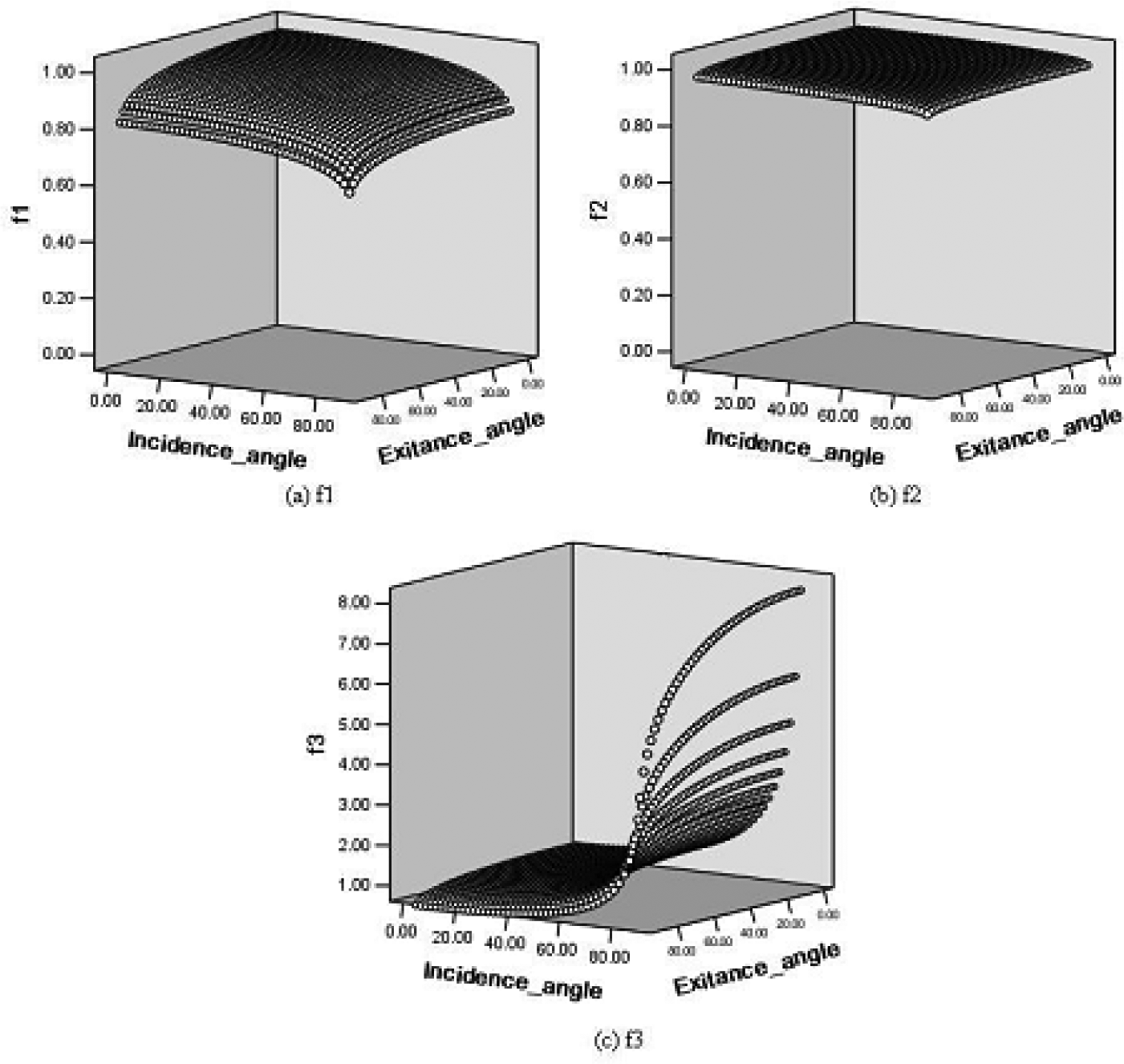
3. Theoretical analysis of topographic effects on EVI and NDVI

To explain theoretically how topography affects the vegetation index, we assume that there exists a pixel Ω, whose slope and aspect are S and A, respectively. Thus, for two given bands 1 and 2 of a sensor, the following equations can be obtained from equation 5:
L T 1 = L O 1 cos e ( cos i cos e ) k 1
L T 2 = L O 2 cos e ( cos i cos e ) k 2
where LO1 and LO2 are the radiance from an inclined surface in bands 1 and 2, respectively; LT1 and LT2 are the normalized radiance in bands 1 and 2; and k1 and k2 are the Minnaert constants for bands 1 and 2. By dividing the two sides of equations 12 and 13 by the incident radiances in the corresponding bands (E1, E2), we can obtain
ρ T 1 = ρ O 1 cos e ( cos i cos e ) k 1
ρ T 2 = ρ O 2 cos e ( cos i cos e ) k 2
By taking the ratio of equations 14 and 15, we can obtain
ρ T 1 ρ T 2 = ρ O 1 ρ O 2 × ( cos i cos e ) k 2 ( cos i cos e ) k 1
which can be rewritten as:
R V I T = R V I O × ( cos i cos e ) k 2 ( cos i cos e ) k 1
where RVI=ρ1/ρ2, and the subscript terms T and O indicate normalized and original vegetation indices.
If the values of the Minnaert constants k for bands blue, red and near-infrared (nir) were derived, we substituted them into the equation 17 and 14, and obtained
ρ nir T ρ red T = R V I T nir red = R V I O nir red ( cos i cos e ) k red k nir
ρ blue T ρ red T R V I T blue red = R V I O blue red ( cos i cos e ) k red k blue
1 ρ red T = R V I T red + R V I O red ( cos i cos e ) k red cos e
where kblue, kred and knir are Minnaert constants of bands blue, red and near-infrared respectively.
Here, we used the following definitions:
f 1 = ( cos i cos e ) k red k blue
f 2 = ( cos i cos e ) k red k nir
f 3 = ( cos i cos e ) k red cos e
Substituting equations 21-23 into equations 2 and 4, we obtained
EVI T = 2.5 ( RVI O nir red × f 2 1 ) RVI O nir red × f 2 + 6 7.5 RVI O blue red × f 1 + RVI O red × f 3
E V I O = 2.5 ( R V I O nir red 1 ) R V I O nir red + 6 7.5 R V I O blue red + R V I O red
NDVI T = RVI O nir red × f 2 1 RVI O nir red × f 2 + 1
NDV I o R V I O nir red 1 R V I O nir red + 1
Equations 24-27 clearly show that f1, f2, and f3 play important roles in determining the relationship between EVIT and EVIO as well as NDVIT and NDVIO. The values of f1, f2 and f3 are determined by the Minnaert constants of bands blue, red and nir. For a Lambertian surface, we have kblue=kred=knir=1, and f1=f2=1, f3=cosi, therefore NDVI0=NDVIT, but EVI0EVIT. That is, there is no topographic effect on the NDVI, which only includes a band ratio format in a Lambertian surface, while the EVI is sensitive topographic effect. For a non-Lambertian surface, if the condition of kred= kblue can be satisfied, we also can consider that the NDVI which only includes the band ratio format is not affected by topography. However, it is much more complicate to consider with EVI, and the Minnaert constants of bands blue, red and nir are needed to analysis the topographic effects on the EVI.

4. A case study for testing topographic effects on EVI and NDVI

4.1. Study area and data processing
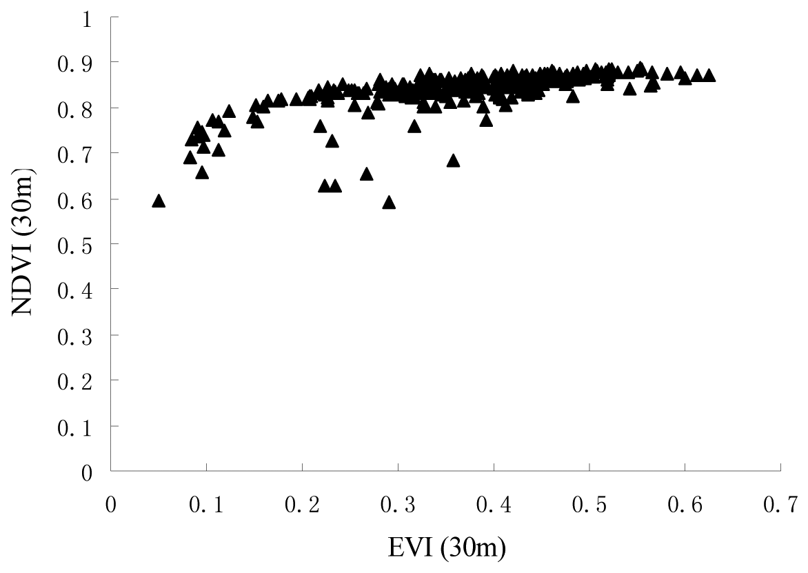
In the 1960s in Japan, Japanese cypress was extensively planted as a major commercial tree species after clear cutting of the pre-existing forest [19-20]. More recently, due to the lack of labor force and the sluggish timber prices, there has been no timely thinning of the high density stands. This has resulted in complete canopy closure, which in turn has prevented the development of understory vegetation strata, leaving the forest floor vulnerable to soil erosion [21]. From the viewpoint of topographic correction and other remote sensing techniques, such areas provide an ideally homogeneous test site, since they consist of trees of the same age and species and have an almost completely closed canopy. The chosen study area (156-watershed), which is located in the Kochi Prefecture in western Japan (Figure 1), is a typical example of such a region. It consists of an area of about 35 ha, and is a typical mountain area, with its highest altitude being 554 m and its lowest altitude 0 m, and its valleys generally run from west to east. Japanese cypress trees were planted here in the 1960s after clear cutting of the pre-existing forest. The stand density is about 2000 stands ha-1 and the canopy is closed. In addition, the values of relative illuminance measured by an illuminometer are almost less than 5% for randomly selected field survey points [22]. Therefore, the study area can be assumed to be uniform.
As pointed out by Trotter (1998), studies of the topographic effect have to date been hindered by a lack of definitive datasets regarding the radiance from hill-country vegetation [12]. The existing datasets contain many sources of variance such as vegetation composition, biomass, and diffuse illumination which are likely to vary with changes in slope, aspect, and altitude, other than those due directly to topography. The complexity of this data makes it difficult to distinguish radiance variations due to topographic effects from those due to other factors. Thus, the spectral data observed in the homogeneous land surface of the study area provides an ideal opportunity to distinguish radiance variations due to topography from those due to other factors, and thus to evaluate topographic effects on the EVI and the NDVI.
Two types of datasets were used in this study. One dataset was derived from a hyperspectral sensor, named AISA (Airborne Imaging Spectrometer for Applications), with 258 narrow contiguous bands ranging from 400 to 2400 nm [23-24]. The bandwidth is approximately 4.08 nm and 11.40 nm over the VNIR and SWIR spectral wavelength ranges, respectively. The AISA data was acquired on September 30, 2004 with a nominal pixel resolution of 1.5×1.5 m (the flight altitude was 1460 m). It was radiometrically corrected to reflectance using the MODTRAN3.7 radiative transfer code, in which the atmospheric water vapor bands of AISA were used to fit the model. The surface reflectance was determined by [25]:
ρ λ = π ( L t , λ L path , λ ) F o , λ T d , λ T o , λ
where ρλ is the reflectance at wavelength λ Lt, λ is the upwelling radiance at the sensor; Lpath,λ is the path radiance; Fo,λ is the exoatmospheric solar irradiance; Td, λ is the downwelling atmospheric transmittance; and To, λ is the upwelling atmospheric transmittance. The NDVI and EVI images were produced from spectral reflectance of bands 17 (central wavelength 466.5 nm), 66 (central wavelength 681.32 nm), and 106 (central wavelength 862.73 nm) of the AISA data using NDVI and EVI definition equations. The other dataset was derived from small-footprint airborne light detection and ranging (LiDAR) data and was used to obtain DEM (Digital Elevation Model) data. The LiDAR data was acquired in March 2004 using an airborne laser scanner operated by the PASCO Corporation. The LiDAR data was then processed to create DEM data with the same spatial resolution and projection as the AISA data
The coefficient of variation (CV) was employed to evaluate the difference between the topographic effects on the EVI and the NDVI. The CV is the standard deviation divided by the mean value, and it has often been used to compare variations within data sets [26]. Since our study area consists of an approximately homogeneous vegetation surface in a mountainous region, it can be considered that the variations of the EVI and the NDVI were due mainly to the topographic differences in this area. That is, the larger CV values were associated with a larger topographic effect and vice versa.

4.2. Results

Figure 2 shows the distribution maps of the aspect, slope, single channel reflectances (i.e., blue, red and near-infrared), EVI, and NDVI in the single flight line of the study area. In the study area, because the understory vegetation strata has disappeared due to the light-blocking forest canopy, the forest canopy in the study area can be considered deep enough to assume a uniform vegetation surface. Therefore, the reflectances of the single channels, especially the blue and red channels, should be saturated and unchanged if in the case of a level surface. However, it can be clearly seen that the reflectance images of the single channels and the EVI image all show a greater variation than does the NDVI image in regard to spatial distribution. The reflectances of the single channels and EVI values are all very different between the north and south aspect, and even within the same aspect area these values also vary among different slopes. In contrast, the NDVI image shows little spatial variation. The results show that the spatial variations of the reflectance in single channels and EVI are all due mainly to the topographic effects, while the NDVI can eliminate or weaken the topographic effects because of its band ratio format. In addition, the CVs of the EVI, NDVI and the slope of this area seen in Figure 2 are 0.28, 0.04 and 0.26, respectively, which also indicates that the EVI is more sensitive to topographic conditions than is the NDVI.
Because the images are too large to be illustrated in 3-D scatter plots, we randomly selected 1000 samples from the images to demonstrate the variations of EVI and NDVI in terms of the different aspects and slopes (Figure 3). It is noted that the NDVI values are approximately 0.8 in any aspect or slope; however, the EVI values vary from 0.1 to 0.5 with the changes of aspects and slopes. The CVs of the EVI and the NDVI shown in Figure 3 are 0.29 and 0.05, respectively, indicating that the topographic effect on the EVI is more significant than that on the NDVI.
In order to find out whether the high spatial resolution of the image (1.5 m) dominated the variations of EVI and NDVI, the original reflectance image was degraded to 30 m, and the EVI and NDVI images were recalculated. There are only 292 pixels obtained because of the small study area. The scatter plot of EVI and NDVI with the resolution of 30 m was shown in Figure 4. It can be seen that the NDVI values are approximately 0.8 in any topography; however, the EVI values vary from 0.1 to 0.6. The CVs of the EVI and the NDVI are 0.3 and 0.05 respectively, indicating that the EVI is more sensitive to topographic effect than NDVI. The characteristics of EVI and NDVI image with middle resolution (30m) were identical with that with high resolution (1.5), which demonstrated that the topographic effect other than high spatial resolution is the major cause of variations in EVI.
To discuss the topographic effect on VIs in the case of a non-Lambertian surface, we need to firstly know the Minnaert constant k. Taking the log of both sides of equation 5 produces a linear from which can be used to estimate k in a linear regression model. That is,
y = k x + b
where, y = log(L0 cos e), b = log(LT), and x = log(cos i cos e). The coefficient k equals the slope of the regression line. Values for k vary as a function of wavelength and surface properties, so that this method is more effective when different k values are applies for different land cover types [10]. However, the present application seeks to develop and test efficient, automated mapping methods, which do not rely on a priori knowledge of land cover types and thus one k value for each spectral band is used for corrections across the entire image [27]. Although the land cover type of the study area is only Japanese cypress plantation, values of k derived form the entire image resulted in low R2 regression values, ranging between 0.03 and 0.11. These low R2 values indicate that the k values would be ineffective for removing the topographic effect [26]. Thus we randomly selected 300 groups of samples, and each group contained 200 pixels. Pixels of each group were used in the linear regression model (equation 29). For every band of AISA data, the k value corresponding with the largest R2 value in the regression procedure among the 300 groups was regarded as the Minnaert constant. As a result, the optimum k values were calculated as 0.15, 0.22, and 0.21, and R2 values are 0.72, 0.59 and 0.67 for the bands 17, 66, and 106 of the AISA data, respectively.
After deriving the values of the Minnaert constant k, we substituted them into the equation 21-23, and obtained
f 1 = ( cos i cos e ) 0.07
f 2 = ( cos i cos e ) 0.01
f 3 = ( cos i cos e ) 0.22 cos e
and,
E V I T = 2.5 ( R V I O nir red × f 2 1 ) R V I O nir red × f 2 + 6 7.5 R V I O blue red × f 1 + R V I O red × f 3
E V I O = 2.5 ( R V I O nir red 1 ) R V I O nir red + 6 7.5 R V I O blue red + R V I O red
NDVI T = RVI O nir red × f 2 1 RVI O nir red × f 2 + 1
NDV I O = R V I O nir red 1 R V I O nir red + 1
Here, we calculated f1, f2, and f3 by using equations 30-32, in which the incidence angle i and exitance angle e changed from 0 to 90 degrees in 2 degree increments, respectively. The results are shown in Figure 5. It is seen that f1 and f2 were always close to 1.0 (Figure 5a and 5b), whereas f3 were far from 1.0 in most cases (Figure 5c). Therefore, the following can be obtained:
NDV I T NDV I O
Whereas
E V I T E V I O
Equation 37 indicates that the NDVI, which only includes a band ratio format, is still not affected by topographic effects even on a non-Lambertian surface. On the other hand, Equation 38 indicates that the topographic effect cannot be neglected in the EVI because of the presence of the soil adjustment factor in the EVI's denominator. Equations 37 and 38 also provide a quasi-quantitative interpretation of Figure 2 and Figure 3. Based on these results, we strongly recommend that the topographic effect be removed from the EVI—as well as from other vegetation indices that similarly include a term without a band ratio format (e.g., PVI: Perpendicular Vegetation Index, [28]; SAVI: Soil Adjusted Vegetation Index, [29]) —when these indices are used in conjunction with a high spatial resolution image of an area of rough terrain, where the topographic effect on the vegetarian indices having only a band ratio format (e.g., the NDVI) can usually be ignored.
Because the Minnaert constants for band Red, Blue and NIR are 0.15, 0.22, and 0.21 respectively, which are quite different from 1.0, the study area should not be regarded as Lambertian surface. Therefore, the indirect effect of topography, which is determined by the BRDF of the surface, cannot be neglected in this study area. As discussed in part 2.2, the direct effect of topography is determined by factor of view-surface normal angle and solar-surface normal angle respectively. For a specific pixel, the view-surface normal angle and solar-surface normal angle are constants for all the bands, thus the ratio vegetation index (RVI) can eliminate the direct effect of topography absolutely. Because the NDVI can be expressed as a function of the RVI, it also can eliminate the direct effect. However, the EVI cannot be written as a function of the RVI because of the soil adjustment factor “L”, so it is much more sensitive to the direct effect than the NDVI. It can be noted that there are still some variations for the NDVI in Figure 2 with CV equals to 0.04, which is mainly induced by the indirect effect. However, the CV of NDVI is much smaller than that of EV (CV equals to 0.28), which demonstrated that the direct effect is larger than the indirect one in the used dataset of this study.

5. Conclusions

The Enhanced Vegetation Index (EVI) was proposed to reduce both atmospheric and soil background noise simultaneously. Although the EVI performs better than does the NDVI in many applications, we have shown in the present paper that it is more sensitive to topographic conditions than is the NDVI. Based on a non-Lambertian model [15,16], we quasi-quantitatively interpreted the reason for the difference of the topographic effect between the EVI and NDVI, and two airborne-based images obtained from a high-density mountain area in Japan were used as a study case to evaluate the conclusion. This study shows that the NDVI can be expressed as a function of the ratio vegetation index (RVI), which can reduce the direct effect of topography absolutely. However, the EVI cannot be written as a function of the RVI because of the soil adjustment factor “L”. Thus, we may conclude that it is the soil adjustment factor in the EVI that makes it much more sensitive to the direct effect than is the NDVI. And both the EVI and NDVI may be influenced by the indirect effect of topography, which is determined by the BRDF of the surface.
Furthermore, we need to be aware that the topographic effect is relative to spatial scale: as the size of the pixel increases, the effect of topography may decrease or even disappear. The quantitative relationship between spatial scale and topographic effect needs further study. Lastly, we strongly recommend that the topographic effect be removed from the EVI—as well as from other vegetation indices that similarly include a term without a band ratio format (e.g., the PVI and SAVI)—when these indices are used in conjunction with a high spatial resolution image of an area of rough terrain, where the topographic effect on the vegetarian indices having only a band ratio format (e.g., the NDVI) can usually be ignored.

Acknowledgments

This study was supported in part by Grants-in-Aid for Scientific Research of MEXT from Japan (No. 17710003) and the CREST project of the JST (No. 2754).

References and Notes

  1. Huete, A.R.; Justice, C. MODIS vegetation index (MOD13) algorithm theoretical basis document. Ver. 3 1999. [Google Scholar]
  2. Liu, H.Q.; Huete, A.R. A feedback based modification of the NDV I to minimize canopy background and atmospheric noise. IEEE Transactions on Geoscience and Remote Sensing 1995, 33, 457–465. [Google Scholar]
  3. Gao, B.C. NDWI - A normalized difference water index for remote sensing of vegetation liquid water from space. Remote Sensing of Environment 1996, 58, 257–266. [Google Scholar]
  4. Soudani, K.; Francois, C.; le Maire, G.; Le Dantec, V.; Dufrene, E. Comparative analysis of IKONOS, SPOT, and ETM+ data for leaf area index estimation in temperate coniferous and deciduous forest stands. Remote Sensing of Environment 2006, 102, 161–175. [Google Scholar]
  5. Nagler, P.L.; Scott, R.L.; Westenburg, C.; Cleverly, J.R.; Glenn, E.P.; Huete, A.R. Evapotranspiration on western US rivers estimated using the Enhanced Vegetation Index from MODIS and data from eddy covariance and Bowen ratio flux towers. Remote Sensing of Environment 2005, 97, 337–351. [Google Scholar]
  6. Boles, S.H.; Xiao, X.M.; Liu, J.Y.; Zhang, Q.Y.; Munkhtuya, S.; Chen, S.Q.; Ojima, D. Land cover characterization of Temperate East Asia using multi-temporal VEGETATION sensor data. Remote Sensing of Environment 2004, 90, 477–489. [Google Scholar]
  7. Xiao, X.; Zhang, Q.; Braswell, B.; Urbanski, S.; Boles, S.; Wofsy, S.; Moore, B.; Ojima, D. Modeling gross primary production of temperate deciduous broadleaf forest using satellite images and climate data. Remote Sensing of Environment 2004, 91, 256–270. [Google Scholar]
  8. Waring, R.H.; Coops, N.C.; Fan, W.; Nightingale, J.M. MODIS enhanced vegetation index predicts tree species richness across forested ecoregions in the contiguous USA. Remote Sensing of Environment 2006, 103, 218–226. [Google Scholar]
  9. Holben, B.N.; Justice, C.O. An examination of spectral band ratioing to reduce the topographic effect on remotely sensed data. International Journal of Remote Sensing 1981, 2, 115–133. [Google Scholar]
  10. Smith, J.A.; Tzeu, L.L.; Ranson, K.J. The Lambertian Assumption and Landsat Data. Photogrammetric Engineering and Remote Sensing 1980, 46, 1183–1189. [Google Scholar]
  11. Meyer, P.; Itten, K.I.; Kellenberger, T.; Sandmeier, S.; Sandmeier, R. Radiometric corrections of topographically induced effects on Landsat TM data in an alpine environment. ISPRS Journal of Photogrammetry and Remote Sensing 1993, 48, 17–28. [Google Scholar]
  12. Trotter, C.M. Characterising the topographic effect at red wavelengths using juvenile conifer canopies. International Journal of Remote Sensing 1998, 19, 2215–2221. [Google Scholar]
  13. Dymond, J.R.; Shepherd, J.D. Correction of the topographic effect in remote sensing. IEEE Transactions on Geoscience and Remote Sensing 1999, 37(2), 2618–2620. [Google Scholar]
  14. Lee, T.Y.; Kaufman, Y.J. Non-lambertian effects on remote sensing of surface reflectance and vegetation index. IEEE Transactions on Geoscience and Remote Sensing 1986, 24, 699–707. [Google Scholar]
  15. Minnaert, M. The Reciprocity Principle in Lunar Photometry. Astrophys Journal 1941, 93, 403–410. [Google Scholar]
  16. Minnaert, M. The Solar System; Kuiper, G.P., Ed.; University of Chicago Press: Chicago, IL, 1961; Volume 3, pp. 213–249. [Google Scholar]
  17. Huete, A.R.; Liu, H.Q.; Batchily, K.; YanLeeuwen, W. A comparison of vegetation indices global set of TM images for EOS-MODIS. Remote Sensing of Environment 1997, 59, 440–451. [Google Scholar]
  18. Rouse, J.W.; Haas, R.H.; Schell, J.A.; Deering, D.W. Monitoring vegetation system in the great plains with ERTS. In Proceedings of the Third Earth Resources Technology Satellite-1 Symposium; Greenbelt, USA; NASASP-351, 1974; pp. 3010–3017. [Google Scholar]
  19. Fukuyama, T.; Takenaka, C. Upward mobilization of 137Cs in surface soils of Chamaecyparis obtusa Sieb. Et Zucc. (hinoki) plantation in Japan. The Science of the Total Environment 2004, 318, 187–195. [Google Scholar]
  20. Onda, Y.; Tsujimura, M.; Nonoda, T.; Takenaka, C. Methods for measuring infiltration rate in forest floor in Hinoki plantations. J. Japan Soc. Hydrol. & Water Resour 2005, 18. [Google Scholar]
  21. Hattori, S.; Abe, T.; Kobayashi, C.; Tamai, K. Effect of forest floor coverage on reduction of soil erosion in hinoki plantations. Bull. For. Prod. Res. Inst 1992, 362, 1–34, (in Japanese, with English summary).. [Google Scholar]
  22. Matsushita, B.; Onda, Y.; Xu, M.; Toyota, M. Detecting forest degradation in Kochi, Japan: Combining in situ field measurements with remote sensing techniques. In IEEE International Geoscience and Remote Sensing Symposium; 2005; 3WE095A_29; pp. 1–4. [Google Scholar]
  23. Mäkisara, K.; Meinander, M.; Rantasuo, M.; Okkonen, J.; Aikio, M.; Sipola, K.; Pylkkö, P.; Braam, B. Airborne imaging spectrometer for applications (AISA). In IGARSS Digest; Tokyo; IGARSS, 1993; pp. 479–481. [Google Scholar]
  24. Mäkisara, K.; AISA Data User's Guide. Technical Research Centre of Finland. Research Note 1894 1998, 1–54. [Google Scholar]
  25. Roberts, D.A.; Green, R.O.; Adams, J.B. Temporal and spatial patterns in vegetation and atmospheric properties from AVIRIS. Remote Sensing of Environment 1997, 62, 223–240. [Google Scholar]
  26. Justice, C.O.; Wharton, S.W.; Holben, B.N. Application of digital terrain data to quantify and reduce the topographic effect on Landsat Data. International Journal of Remote Sensing 1981, 2, 213–230. [Google Scholar]
  27. Carpenter, G.A.; Gopal, S.; Macomber, S.; Martens, S.; Woodcock, C.E. A Neural Network Method for Mixture Estimation for Vegetation Mapping. Remote Sensing of Environment 1999, 70, 139–152. [Google Scholar]
  28. Baret, F.; Guyot, G. Potentials and limits of vegetation indices for LAI and APAR assessment. Remote Sensing of Environment 1991, 35, 161–173. [Google Scholar]
  29. Huete, A.R. A soil adjusted vegetation index (SAVI). Remote sensing of Environment 1988, 25, 295–309. [Google Scholar]
Figure 1. The study area and its landscape.
Sensors 07 02636f1
Figure 2. The spatial distribution of aspect, slope, single channel reflectances (blue, red and near-infrared), EVI and NDVI in the study area.
Sensors 07 02636f2
Figure 3. 3-D Scatter plots of NDVI and EVI of randomly selected 1000 samples from the image.
Sensors 07 02636f3
Figure 4. Scatter plot of EVI and NDVI after the image was resampled to 30m.
Sensors 07 02636f4
Figure 5. The distributions of values of f1, f2, and f3.
Sensors 07 02636f5

