Modeling Volatility Characteristics of Epileptic EEGs using GARCH Models

1
Department of Mathematics and Computer Science, University of St. Thomas, 3800 Montrose Boulevard, Houston, TX 77006, USA
2
Division of Biostatistics and Data Science, The University of Texas Health Science Center at Houston, School of Public Health, 1200 Herman Pressler Drive, W-1006, Houston, TX 77030, USA
*
Author to whom correspondence should be addressed.
Signals 2020, 1(1), 26-46; https://0-doi-org.brum.beds.ac.uk/10.3390/signals1010003
Submission received: 18 February 2020
/
Revised: 21 May 2020
/
Accepted: 27 May 2020
/
Published: 2 June 2020
Abstract
:Objective: To determine if there was a difference in the volatility characteristics of seizure and non-seizure onset channels in the intracranial electroencephalogram (EEG) in a patient with temporal lobe epilepsy. Methods: The half-life of volatility for the different EEG channels was determined using Autoregressive Moving Average–Generalized Autoregressive Conditional Heteroscedasticity (ARMA–GARCH) models; confidence intervals were constructed using the delta method and an asymptotic method for comparing the half-lives. Results: Clinically determined seizure onsets occurred over strip electrodes named RAST (Right Anterior Subtemporal) and RMST (Right Mid Subtemporal), at locations 2, 3 and 4, on the strip electrodes. The half-lives of volatility for two of the three seizure channels, RAST3 and RAST4, were found to be significantly lower the rest of the channels for six one-minute EEG segments prior to seizure onset and nine one-minute EEG segments of an awake state. The half-lives of volatility for RAST3 and RAST4 were not significantly different to the non-seizure channels for ten one-minute segments of sleep and ten one-minute segments of sleep-to-awake states. The estimates for the half-lives were consistent for randomly selected one-minute EEG segments. Conclusions: The use of GARCH models may be a useful tool in determining hidden properties in epileptiform EEGs that may lead to better understanding of the seizure generating process.
1. Introduction
The visual examination of electroencephalograms (EEGs) is limited by potential subjectivity due to limited protocols and the inability to identify hidden patterns, characteristics or relationships in large amounts of data [1,2]. The introduction of quantitative methods in the analysis of EEGs attempt to overcome these limitations by introducing objective measures of EEG characteristics [1]. These methods give both the clinician and/or researcher access to the valuable information within the EEG concerning the dynamics of brain activity. Much of the quantitative research in epilepsy is based on the detection of changes (spikes, spike-waves, sharp waves, etc.,) in the properties of an EEG; the changes in the waveforms are associated with changes in behavioral and mental states. During an epileptic seizure, the EEG exhibits robust changes [3,4]. The amplitude of the EEG increases during an epileptic seizure due to episodic brief neuronal synchronous discharges; the seizure at onset may be seen in only a few EEG channels (local or partial seizure) or in all EEG channels (generalized seizure) [2]. The information obtained from EEGs using quantitative methods has been used in such areas as attempting to predict/anticipate the occurrence of seizures, attempting to detect the onset/occurrence of seizures, and in modeling seizure propagation/dynamics.
The EEG, like many physiological time series, is widely believed to be non-stationary due to its time-varying properties; the non-stationarity may arise from the fact that the observation time is shorter than the characteristic time scale of the EEG [3]. The non-stationarity of the EEG limits the use of classical time series analysis methods. However, early attempts at analyzing EEG signals in the time domain were based on a linear approach using autoregressive moving average (ARMA) modeling [5]. Even though the use of ARMA models in the analysis of EEG signals is limited because of the EEG’s time-varying properties, their usage contributed to the understanding of EEG signals [6]. Mormann et al. [7], citing studies by Rogowski et al., Salant et al., and Siegal et al., found changes in the autoregressive parameters seconds prior to the onset of a seizure as well as differences in characteristics between one-minute epochs prior to a seizure and control subjects. There are also studies on characterization of EEG time series using spectral and wavelet analysis [8,9,10,11,12,13,14].
Some EEG analyses have moved away from linear time series analysis methods and toward the use of non-linear time series analysis. Measures such as Lyapunov exponents, correlation dimension, correlation density, entropy, and dynamic similarity have been employed [15,16,17,18,19,20,21,22,23,24,25,26,27,28]. Additional techniques that have been used in quantitative EEG analysis either alone or combined with other methods include, but are not limited to, spatial-temporal modeling, wavelets, genetic algorithms, data mining, morphological filters, discriminant analysis, neural networks and support vector machines [29,30,31,32,33,34,35,36,37,38,39,40,41,42,43,44]. Convolutional Neural Networks have also been used for feature classification and seizure detection [45,46,47,48]. Recent research has also focused on high-frequency oscillations (HFOs) in epileptic EEGs [45,48,49,50,51,52,53]
While the above listed methods have been used in EEG analysis, the use of GARCH models in characterizing volatility has not been explored. Conditional volatility models originated in finance with the ARCH (autoregressive conditional heteroscedastistic) model of Engle and the GARCH (generalized autoregressive conditional heteroscedastistic) model of Bollerslev [54,55]. These models and their extensions have been used to characterize the temporal behavior and clustering of volatility in financial markets. The use of these models to characterize the volatility of epileptiform EEG signals may be able to provide more insight into the seizure generating processes, may be used in identifying epileptogenic zones, and may have use in the prediction of seizures as well as aid in a diagnosis of epilepsy. In this study, volatility characteristics of epileptiform EEGs were examined for possible differences between seizure and non-seizure onset channels using GARCH models.
2. Methods
Data
The data used in this study were provided by the Department of Neurology at the University of Texas McGovern Medical School. Four epochs of intracranial EEG (awake, sleep, sleep to awake, and seizure) sampled at 200 Hz over various parts of the right hemisphere of a single individual’s brain were used in the analysis. The recordings were obtained from subdural grid and strip electrodes, placed directly over the brain surface through an operative procedure for the clinical investigation of temporal lobe epilepsy. The grids and strip electrodes were recorded from a total of sixty-six discrete channels over different brain regions. In the days following electrode placement, seizures were identified over contacts 2 and 3 on the strip electrode labeled RAST (Right Anterior Subtemporal) and over contact 4 on the strip electrode labeled RMST (Right Mid Subtemporal). The awake, sleep, and sleep to awake segments were approximately 10 min in length, with waking occurring in the sleep to wake signal at approximately 8 min; the segment with the seizure was approximately 15.5 min in length, with six minutes of pre-seizure data, 2.5 min of seizure data and seven minutes of post-seizure data. The onset of seizure was determined by conventional visual analysis by a clinical neurologist. All four segments were referenced to an external zero voltage reference. The data used in the analyses were de-identified.
3. Conditional Volatility Models
3.1. Autoregressive Moving Average Models
One of the traditional models used in modeling the dynamics of a time series is the Autoregressive Moving Average (ARMA) process. ARMA(p,q) processes are stationary. For stationary processes, the characteristics of the distribution for a sequence of observations are not dependent on the time origin [56]. A less restrictive requirement is that of a weakly stationary process, where, for a time series , for all , for all , and for , where is the autocorrelation function of a time series; thus, for a weakly stationary time series, the mean and variance are constant and the correlation between observations is only dependent on the time between the observations [56]. The property of weak stationarity is often employed in the analysis of time series [56]. Processes of the form under commonly used conditions
where is a white noise sequence with variance for all (for time series with non-zero mean, a mean term can be added to the model) [56,57].
If or , then the processes are described as a moving average process of order q (MA(q)) or an autoregressive process of order (AR(p)) respectively. If a time series is non-stationary, Autoregressive Integrated Moving Average (ARIMA(p,d,q)) models may be used, where the dth difference of the time series is an ARMA(p,q) process [56]. The parameters of an ARMA model are useful in summarizing a time series, while the modeling may not reveal much information concerning the data generating process; however, ARMA processes are useful in forecasting [57].
3.2. Generalized Autoregressive Conditional Heteroscedasticity Models
One limitation of an ARMA model is the assumption of constant conditional variance ( where is the set of information available at time , mathematically, a σ-field generated from {Yt-1, Yt-2,…}), and, thus, is not satisfactory for use in modeling time series with time varying variance [56]. Variance that changes of over time may affect the inferential validity and efficiency of the parameters of an ARMA model [58]. Models that account conditionally for non-constant volatility (non-constant conditional variance) allow for better predictions of (local) variability and better prediction intervals [59]. Time series with non-constant volatility are common in finance, and the most common family of volatility models were developed to model financial time series; their use in biomedical research has been rarely utilized [60,61,62].
The Autoregressive Conditional Heteroscedasticity (ARCH) model was developed by Engle and generalized (GARCH) by Bollerslev [54,55]. The GARCH(p,q) model for a time series is
where is the expectation conditional on information available at time , are i.i.d. zero mean random variables with unit variance, , and
[63].
These constraints ensure positive and finite unconditional variance for , with a necessary and sufficient condition for weak stationarity. A less restrictive necessary and sufficient condition for strict stationarity is that , with certain conditions on the . This allows the sum to equal or exceed one [55,64,65,66]. The , often referred to as ‘shocks,’ are serially uncorrelated, but dependent. The and in the conditional variance equation are the ARCH and GARCH parameters respectively, with and the unconditional variance of is
which will be positive due to the constraints. A GARCH model with is an ARCH(p) model and in order to identify the parameters, and are co-primes [67].
If the conditional variance equation follows an ARCH(1) process, , large values of result in a larger deviation from , and the conditional variance of is larger as a result. This volatility will propagate since a large deviation of makes and large (similarly for small values of ). Thus, the volatility will persist, but will eventually revert to the unconditional variance since . For ARCH(p) processes, large past shocks lead to a large conditional variance for and a large value of . Thus, the probability of a large shock following a large shock is greater than the probability of small shock. This leads to the volatility clustering often seen in financial time series [56,68].
The development of GARCH(p,q) models were motivated by the shortcomings in the ARCH(p) models and provide more flexibility than ARCH(p) models. Some weaknesses of an ARCH(p) model are that the order p may be high (leading to the need for estimating many parameters), that it is likely to overpredict the volatility, that it does not capture the excess kurtosis seen in financial time series, and that it assumes that positive and negative shocks produce the same effect on volatility [68]. ARCH(p) models also have high volatility in short bursts, or short volatility persistence, while GARCH() models allow for more persistent volatility [56]. GARCH processes also tend to have heavy tails and GARCH models also tend to be more parsimonious, and the simplest form, GARCH(), has been successful in predicting conditional volatility [56,69]. GARCH models may be used to model the innovations of ARMA models (ARMA–GARCH) as well.
For a GARCH() model, values of closer to 1 produce a high correlation between and which allows for longer persistence of volatility than an ARCH(1) model [68]. The speed with which the process reverts to the unconditional variance (persistence) is governed by the magnitude of [63]. The half-life (HL) of a volatility shock, a measure of the length of time it takes for a shock to decrease by one-half, is given by , and as approaches 1, the larger the half-life [63]. Models for which also imply longer volatility persistence [56]. These results can be extended to higher order GARCH() models [63].
4. Confidence Intervals for Half-Life (HL)
To construct conventional two-sided confidence intervals, the standard errors for the half-life can be approximated using the delta method and using the large sample asymptotic properties of the estimated parameters. Using the delta method, the variance of a differentiable function of random variables, , where , can be approximated as
where
and
Using the equation for half-life, , for a GARCH (1,1) model, taking partial derivatives and substituting into the variance equation above yields the following equation for the standard error:
Based on large sample asymptotics, the confidence interval for the half-life can be constructed as:
Additionally, using the fact that the variance of the sum of random variables is the sum of the variances plus the sums of twice the respective covariances, confidence intervals can also be constructed for the sum of the coefficients. The 95% confidence intervals for large sample sizes can be constructed as:
where Z is the sum of n random variables. The estimates for the upper and lower confidence limits can then be transformed using the half-life formula since it is a monotonic function in order to obtain a confidence interval for the half-life.
5. Analysis
All four datasets were divided into one-minute (12,000 values) segments for analysis. This resulted in 15 segments for the seizure data, 10 segments for the sleep and sleep to awake data, and 9 segments for the awake data. Of the 15 segments for the seizure data, there were six complete segments preceding seizure onset, one segment containing seizure onset, one segment of seizure, one segment containing the transition from ictal to post-seizure, and six post-seizure segments. The sleep-to-awake data had seven segments of sleep data, one segment containing the transition from sleep to awake and two segments of awake data. For each segment, ARMA–GARCH models were estimated for all 66 channels using MATLAB. The estimated parameters from the models were used to estimate unconditional volatility and half-lives. Confidence intervals for half-lives based on the GARCH coefficients were constructed. Additionally, models were estimated for one-minute segments with randomly selected starting points to see if the models were dependent on the particular segments.
6. Results
The onset of the seizure was identified at the three channels RAST3, RAST4 and RMST4. Based on these three channels, the ARMA(2,2)–GARCH(1,1) models were estimated for all channels. Using Equations (1) and (2), these models take the following form where is the value of EEG signal i at time t:
where and
Models were estimated for all segments of the seizure data. The models based on the seizure and post-seizure resulted in integrated models; thus, results only for the pre-seizure data are included. For the other three datasets, models were estimated for all segments.
The models used to estimate and examine volatility were ARMA(2,2)-GARCH(1,1) models. Since the EEG is believed to be non-stationary, one-minute (12,000 points) segments were selected and assumed to be (weakly) stationary. This particular model was selected for this analysis based on fitting an ARMA(2,2) model to the data, and checking the innovations (errors) for heteroscedasticity using an Ljung–Box Q test, and examining the autocorrelation and partial autocorrelation plots for GARCH characteristics, namely serial correlation in the squared innovations. These models were initially fit to the three seizure channels (RAST3, RAST4 and RMST4) and the standardized residuals were tested using the Ljung–Box Q test.
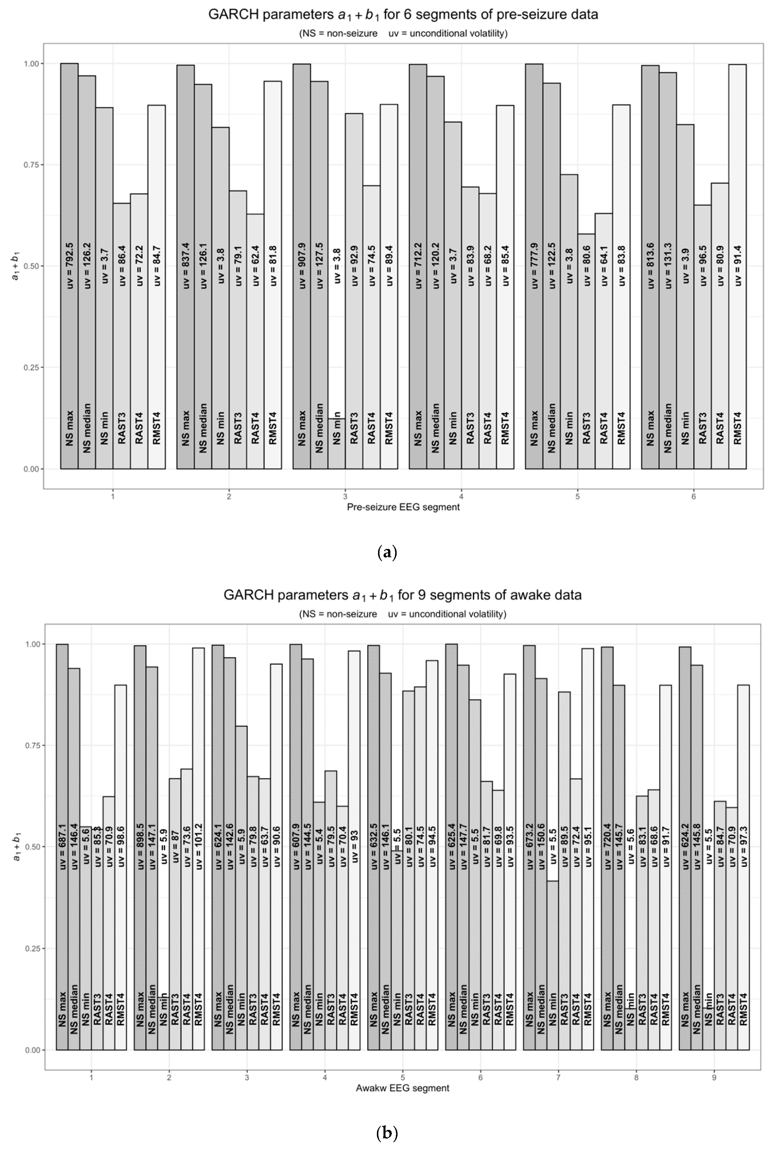
In addition to testing the standardized residuals, the fit of the GARCH(1,1) model to innovations of the ARMA(2,2) model, the estimated unconditional volatility from the GARCH coefficients and the variance of the innovations are listed in Figure 1a–d (all coefficients for models are included in supplementary Table S1a–d). For the three seizure channels, unconditional volatility estimates were within two percent of the innovation variance, with the exception of segment 3 of RAST3, which showed an approximate seven percent difference; this particular channel also had the highest estimated GARCH coefficient (0.7485) and coefficient sum (0.8763). The data for the other signals showed similar results with RAST3 awake segment 7, sleep to awake segment 3, sleep segments 1 and 3, RAST4 awake segment 5 and RMST4 sleep segments 1, 3, and 5 showing greater than five percent difference. For the other channels, three from the seizure data, fifteen from the awake data, twenty-two from the sleep to awake data and ninety from the sleep data had a greater than five percent difference between unconditional volatility and innovation variance.
6.1. GARCH Models
The estimated GARCH coefficients and unconditional volatilities for RAST3, RAST4 and RMST4 are listed in Table 1a–d, along with the minimum, median and maximum of the coefficients from the non-seizure channels. Table 1a shows the results for six one-minute segments preceding the onset of seizure. RAST3 and RAST4 show higher ARCH and lower GARCH parameters across all segments than the majority of the other signals; the sum of the ARCH and GARCH parameters are also lower than the majority of the other channels. Estimates for RMST4 do not appear to be different than the non-seizure channels. The unconditional volatility for all three channels do not show as marked a difference; however, each are less than the median of the unconditional volatility of all other signals for each segment. Similar results can be seen for the awake data (Table 1b). As with the seizure data, RAST3 and RAST4 show higher ARCH and lower GARCH coefficients than RMST4 and all of the other channels. The unconditional volatility for each of the three channels is also lower than the median for the other channels. The sleep to awake and sleep data (Table 1c,d) do not show as large of differences as the seizure and awake data. The estimated ARCH and GARCH coefficients of the sleep to awake and sleep data for RAST3 and RAST4 are higher (lower) than the median for the non-seizure channels. The unconditional volatility for the three channels are also lower than the median for the non-seizure channels and are similar to the those found in the seizure and awake data.
For the seizure data, the estimates across the six segments for the seizure channels for RAST3 show the most variation. RAST3 ranges from 0.4449 to 0.7485 for the GARCH coefficient, while the estimates for the ARCH coefficient only range from 0.1145 to 0.1516; the sum of the coefficients has a maximum of 0.8763 in the third segment, while the other sums are relatively similar. The unconditional volatility has a range of 79.1 to 96.5. The variation of the estimates for RAST4 and RMST4 do not show as large of differences as RAST3. The coefficients for RAST4 are similar across all segments; however, the unconditional volatility ranges from 62.4 to 80.9. RMST4 shows similar estimates across the first five segments, with noticeable differences in the sixth segment for the GARCH estimate. All three channels show jumps in unconditional volatility from the fifth to the sixth segment.
The estimates across the nine segments of the awake data do not show as much variation. Segments 5 and 7 for RAST3 and segment 5 for RAST4 have higher GARCH coefficients and higher coefficient sums than the estimates for the other segments. The unconditional variation is similar across all segments for all three channels. For the sleep to awake data, the estimates are similar across the segments with the exception of the unconditional volatility for segment 9 (first awake only segment) of RAST3 and RAST4. All three channels have their minimum unconditional volatility in the last segment. The sleep data estimates are similar across all segments.
6.2. Half-life and Confidence Intervals
To examine the volatility across all channels for the different segments of each dataset, the volatility half-life was calculated for each model along with 95% confidence intervals using the delta and asymptotic methods outlined above (Equations (6) and (7)). Only models with both significant ARCH and GARCH coefficients were used, and confidence intervals with negative confidence limits were used.
There were noticeable differences between the seizure and non-seizure channels in the pre-seizure and awake datasets (Table 1a,b and Table 2a,b). The half-life estimates for RAST3 and RAST4 were between one and two for all but three segments of the both datasets, indicating a volatility persisting half as long as most other channels, and at least four times shorter than at least half of all other channels. In examining the CIs for these two channels, they overlap with at most five of the CIs of the non-seizure channels using the delta method (Table 2a,b) and at most one using the asymptotic method (except for the segments where the half-life was greater than 2). For RMST4, the half-life for the segments varied, ranging from 6.33 to 268.82, with more than half below 6.50; the CIs for these overlapped more than half of the CIs for the non-seizure channels for all of the awake segments and approximately half for the pre-seizure data (for both methods). The CIs for RMST4 only overlapped the CIs of RAST3 and RAST4 in segment 6 of the pre-seizure data using the delta method.
For the sleep and sleep to awake data, the half-life estimates are higher than the pre-seizure and awake data for all channels (Table 2c,d). The half-life CIs for RAST3 and RAST4 overlap a greater number of non-seizure CIs in both datasets; however, in the sleep to awake data, both channels overlap approximately half of the non-seizure CIs. The half-life values appear to be highest in the sleep data relative to the other three datasets. For the non-seizure channels, the median half-life is higher for all segments in both datasets, with the exception of the last segment of the sleep to awake data (Table 2d). This particular segment is the second segment of awake data in the sleep to awake segment and has a median half-life of 14.58, which is similar to the values for the segments of the awake data. Similar behavior is seen for RMST4, which has similar half-life values to the awake data, but not in RAST3 and RAST4, which both have half-life values greater than the median.
7. Random Starting Points
To assess whether the estimated models were dependent on the particular segment, 100 models based on randomly selected starting points within each dataset were estimated for all 66 channels and sample statistics calculated (Table 3). The average half-life for RAST3 (2.25 vs. 2.11) and RAST4 (1.75 vs. 1.86) were similar to the average of the half-life from the six pre-seizure segments. The third quartile score for each signal was also less than two; all half-life estimates for both channels were lower than 75% of the estimates for the non-seizure channels. RMST4 had higher estimates than the other two channels and at least 75% of the scores fell below the median for non-seizure channels. Similar results can be seen for the awake data. For the sleep to awake and sleep data, the estimates are lower on average, but without as large or noticeable differences as seen in the pre-seizure and awake data.
8. Discussion
In examining the volatility of EEG signals, two of the three channels where seizures originated (RAST3 and RAST4) had shorter volatility half-life relative to all other channels in the time leading up to the seizure (6 min) and during an awake state. During a sleep state and a sleep-to-awake state, the volatility half-life for the seizure channels were lower for most segments examined, but the respective confidence intervals (constructed from both methods) overlapped a larger proportion of non-seizure confidence intervals. The volatility also tended to persist longer in the sleep state than in the pre-seizure and awake states, but the half-life varied more than in the pre-seizure and awake data. The volatility half-life was similar to the non-seizure channels, especially in the awake data; however, for the sleep data, the half-lives were lower for half the segments.
For all of the models, the GARCH coefficient was larger than the ARCH coefficient, indicating larger volatility persistence. However, for some of models, the magnitudes of the coefficients could be an issue. While the coefficients were significant at the 5% level, some of the models had GARCH coefficients greater than 0.95 and ARCH coefficients smaller 0.01. The small ARCH coefficients make the effect of the past innovations negligible, which is an issue since GARCH models must have at least one non-zero ARCH parameter for the GARCH parameters to be identified. Additionally, the sum of the coefficients was greater than 0.99 (but less than 1.00), which is very close to being an integrated model. These extreme cases may indicate structural changes occurring in the signals during the one-minute interval, and a more dynamic model may be more appropriate.
The estimated confidence intervals for RAST3 and RAST4 constructed by both methods were similar for all datasets; however, the confidence limits were more in agreement when the half-life estimates were smaller (<10). The CIs for RMST4 were wider for similar half-life estimates, indicating higher variability in the RMST4 estimates. The non-seizure channels also had higher variability, leading to exclusion of some CIs because of negative confidence limits. It appears larger half-life estimates yield much wider CIs. This may be due to a higher covariance between the ARCH and GARCH parameters as their difference grows and/or their sum approaches unity.
The models estimated were based on one-minute segments of data, assuming that they were stationary, which may not be the case. However, in the cases of RAST3 and RAST4, it appears that the models were consistent across different segments for the pre-seizure and awake data, both in the segments used in the analyses and when randomly selecting starting points. This may indicate that these signals are ARMA–GARCH processes for these particular states. The differences in the estimates for the sleep and sleep to awake data may also be indicative of an underlying ARMA–GARCH structure, but they may have different lag structures. The non-seizure signals may also be ARMA–GARCH processes with different lag structures, especially the cases where the ARCH parameter was less than 0.01. All of the signals may also show different volatility properties with shorter segments, indicating possible regime changes.
The volatility half-life as a characteristic of epileptic EEG channels may be related to high frequency oscillations (HFOs), which may be possible characteristics in epileptic EEG channels ([48]. HFOs and their relationship to seizure onset zones have been studied using machine learning and deep learning methods [48,49,50,52,70]. These studies have found various accuracy, sensitivity and specificity in identifying under different conditions, but do pose another potential tool in studying EEGs.
9. Conclusions
To conclude, the use of ARMA–GARCH models to explore the volatility in the human EEG shows promise as a method of identifying otherwise unobservable properties in the signals. In particular, we suggest that identification of volatility properties may help in qualifying seizure dynamics.
This study modeled the innovations as GARCH(1,1) processes, which may be too simplistic—other types of GARCH models may be appropriate, possibly an Integrated GARCH (IGARCH) model, or one that takes leverage effects into account. Multivariate ARMA–GARCH models may also be considered since the signals may be correlated. Other models for estimating volatility may also be used, such as stochastic volatility models.
Supplementary Materials
The following are available online at https://0-www-mdpi-com.brum.beds.ac.uk/2624-6120/1/1/3/s1, Table S1a: GARCH parameters for 6 segments of pre-seizure data; Table S1b: GARCH parameters for 9 segments of awake data; Table S1c: GARCH parameters for 10 segments sleep-to-awake data; Table S1d: GARCH parameters for 10 segments of sleep data.
Author Contributions
J.L.F. conducted statistical analyses, created tables and graphs, and contributed to writing and editing of the manuscript. D.L. contributed to the writing and editing of the manuscript and provided project oversight. All authors have read and agreed to the published version of the manuscript.
Funding
This research received no external funding.
Acknowledgments
The authors would like to thank Giridhar Kalamangalam, Department of Neurology, College of Medicine, University of Florida Health, for providing the data used in this study.
Conflicts of Interest
The authors declare no conflict of interest.
References
- Rosso, O.A.; Martin, M.; Plastino, A. Brain electrical activity analysis using wavelet-based informational tools. Phys. A Stat. Mech. Appl. 2002, 313, 587–608. [Google Scholar] [CrossRef]
- Adeli, H.; Zhou, Z.; Dadmehr, N. Analysis of EEG records in an epileptic patient using wavelet transform. J. Neurosci. Methods 2003, 123, 69–87. [Google Scholar] [CrossRef]
- Dikanev, T.; Smirnov, D.; Wennberg, R.; Velazquez, J.P.; Bezruchko, B. EEG nonstationarity during intracranially recorded seizures: Statistical and dynamical analysis. Clin. Neurophysiol. 2005, 116, 1796–1807. [Google Scholar] [CrossRef] [PubMed]
- Senhadji, L.; Wendling, F. Epileptic transient detection: Wavelets and time-frequency approaches. Neurophysiol. Clin. Neurophysiol. 2002, 32, 175–192. [Google Scholar] [CrossRef] [Green Version]
- Lehnertz, K.; Mormann, F.; Osterhage, H.; Müller, A.; Prusseit, J.; Chernihovskyi, A.; Staniek, M.; Krug, D.; Bialonski, S.; Elger, C.E. State-of-the-Art of Seizure Prediction. J. Clin. Neurophysiol. 2007, 24, 147–153. [Google Scholar] [CrossRef] [PubMed]
- Osterhage, H.; Lehnertz, K. NONLINEAR TIME SERIES ANALYSIS IN EPILEPSY. Int. J. Bifurc. Chaos 2007, 17, 3305–3323. [Google Scholar] [CrossRef]
- Mormann, F.; Andrzejak, R.G.; Elger, C.E.; Lehnertz, K. Seizure prediction: The long and winding road. Brain 2007, 130, 314–333. [Google Scholar] [CrossRef] [Green Version]
- Acharya, U.R.; Sree, S.V.; Ang, P.C.A.; Yanti, R.; Suri, J.S. Application of Non-Linear and Wavelet Based Features for the Automated Identification of Epileptic Eeg Signals. Int. J. Neural Syst. 2012, 22, 1250002. [Google Scholar] [CrossRef]
- Ahammad, N.; Fathima, T.; Joseph, P. Detection of Epileptic Seizure Event and Onset Using EEG. BioMed Res. Int. 2014, 2014, 1–7. [Google Scholar] [CrossRef]
- Faust, O.; Acharya, U.R.; Adeli, H.; Adeli, A. Wavelet-based EEG processing for computer-aided seizure detection and epilepsy diagnosis. Seizure 2015, 26, 56–64. [Google Scholar] [CrossRef] [Green Version]
- Urigüen, J.A.; Garcia-Zapirain, B.; Artieda, J.; Iriarte, J.; Valencia, M. Comparison of background EEG activity of different groups of patients with idiopathic epilepsy using Shannon spectral entropy and cluster-based permutation statistical testing. PLoS ONE 2017, 12, e0184044. [Google Scholar] [CrossRef] [PubMed] [Green Version]
- Jun, Y.-H.; Eom, T.-H.; Kim, Y.-H.; Chung, S.-Y.; Lee, I.G.; Kim, J.-M. Changes in background electroencephalographic activity in benign childhood epilepsy with centrotemporal spikes after oxcarbazepine treatment: A standardized low-resolution brain electromagnetic tomography (sLORETA) study. BMC Neurol. 2019, 19, 3. [Google Scholar] [CrossRef] [PubMed]
- Hu, D.; Cao, J.; Lai, X.; Liu, J. Epileptic State Classification based on Intrinsic Mode Function and Wavelet Packet Decomposition. In Proceedings of the 2019 41st Annual International Conference of the IEEE Engineering in Medicine and Biology Society (EMBC), Berlin, Germany, 23–27 July 2019; pp. 2382–2385. [Google Scholar]
- Swami, P.; Bhatia, M.; Tripathi, M.; Chandra, P.S.; Panigrahi, B.K.; Gandhi, T.K. Selection of optimum frequency bands for detection of epileptiform patterns. Healthc. Technol. Lett. 2019, 6, 126–131. [Google Scholar] [CrossRef] [PubMed]
- Mormann, F.; Lehnertz, K.; David, P.; Elger, C.E. Mean phase coherence as a measure for phase synchronization and its application to the EEG of epilepsy patients. Phys. D Nonlinear Phenom. 2000, 144, 358–369. [Google Scholar] [CrossRef]
- Le Van Quyen, M.; Martinerie, J.; Navarro, V.; Baulac, M.; Varela, F.J. Characterizing Neurodynamic Changes Before Seizures. J. Clin. Neurophysiol. 2001, 18, 191–208. [Google Scholar] [CrossRef]
- Aschenbrenner-Scheibe, R.; Maiwald, T.; Winterhalder, M.; Voss, H.U.; Timmer, J.; Schulze-Bonhage, A. How well can epileptic seizures be predicted? An evaluation of a nonlinear method. Brain 2003, 126, 2616–2626. [Google Scholar] [CrossRef] [Green Version]
- Li, D.; Zhou, W.; Drury, I.; Savit, R. Non-linear, non-invasive method for seizure anticipation in focal epilepsy. Math. Biosci. 2003, 186, 63–77. [Google Scholar] [CrossRef]
- Mormann, F.; Kreuz, T.; Andrzejak, R.G.; David, P.; Lehnertz, K.; Elger, C.E. Epileptic seizures are preceded by a decrease in synchronization. Epilepsy Res. 2003, 53, 173–185. [Google Scholar] [CrossRef]
- Pardalos, P.M.; Chaovalitwongse, W.; Iasemidis, L.D.; Sackellares, J.C.; Shiau, D.-S.; Carney, P.R.; Prokopyev, O.A.; Yatsenko, V.A. Seizure warning algorithm based on optimization and nonlinear dynamics. Math. Program. 2004, 101, 365–385. [Google Scholar] [CrossRef]
- Bartolomei, F.; Wendling, F.; Regis, J.; Gavaret, M.; Guye, M.; Chauvel, P. Pre-ictal synchronicity in limbic networks of mesial temporal lobe epilepsy. Epilepsy Res. 2004, 61, 89–104. [Google Scholar] [CrossRef]
- Escalona-Morán, M.; Cosenza, M.G.; Guillén, P.; Coutin, P. Synchronization and clustering in electroencephalographic signals. Chaos Solitons Fractals 2007, 31, 820–825. [Google Scholar] [CrossRef] [Green Version]
- Iasemidis, L.; Shiau, D.-S.; Pardalos, P.; Chaovalitwongse, W.; Narayanan, K.; Prasad, A.; Tsakalis, K.; Carney, P.; Sackellares, J. Long-term prospective on-line real-time seizure prediction. Clin. Neurophysiol. 2005, 116, 532–544. [Google Scholar] [CrossRef] [PubMed]
- Kannathal, N.; Choo, M.L.; Acharya, U.R.; Sadasivan, P. Entropies for detection of epilepsy in EEG. Comput. Methods Programs Biomed. 2005, 80, 187–194. [Google Scholar] [CrossRef] [PubMed]
- Kaplan, A.Y.; Fingelkurts, A.A.; Borisov, S.V.; Darkhovsky, B.S. Nonstationary nature of the brain activity as revealed by EEG/MED: Methodological, practical and conceptual challenges. Signal Process. 2005, 85, 2190–2212. [Google Scholar] [CrossRef]
- Le Van Quyen, M.; Soss, J.; Navarro, V.; Robertson, R.; Chávez, M.; Baulac, M.; Martinerie, J. Preictal state identification by synchronization changes in long-term intracranial EEG recordings. Clin. Neurophysiol. 2005, 116, 559–568. [Google Scholar] [CrossRef] [PubMed]
- Li, X.; Ouyang, G. Nonlinear similarity analysis for epileptic seizures prediction. Nonlinear Anal. Theory Methods Appl. 2006, 64, 1666–1678. [Google Scholar] [CrossRef]
- Winterhalder, M.; Schelter, B.; Maiwald, T.; Brandt, A.; Schad, A.; Schulze-Bonhage, A.; Timmer, J. Spatio-temporal patient–individual assessment of synchronization changes for epileptic seizure prediction. Clin. Neurophysiol. 2006, 117, 2399–2413. [Google Scholar] [CrossRef]
- Wendling, F.; Bartolomei, F.; Bellanger, J.; Chauvel, P. Interpretation of interdependencies in epileptic signals using a macroscopic physiological model of the EEG. Clin. Neurophysiol. 2001, 112, 1201–1218. [Google Scholar] [CrossRef]
- Jouny, C.; Franaszczuk, P.J.; Bergey, G.K. Characterization of epileptic seizure dynamics using Gabor atom density. Clin. Neurophysiol. 2003, 114, 426–437. [Google Scholar] [CrossRef]
- Kiymik, M.K.; Subasi, A.; Ozcalık, H.R. Neural Networks with Periodogram and Autoregressive Spectral Analysis Methods in Detection of Epileptic Seizure. J. Med. Syst. 2004, 28, 511–522. [Google Scholar] [CrossRef]
- Shoeb, A.; Edwards, H.; Connolly, J.; Bourgeois, B.; Treves, S.T.; Guttag, J. Patient-specific seizure onset detection. Epilepsy Behav. 2004, 5, 483–498. [Google Scholar] [CrossRef] [PubMed] [Green Version]
- Alkan, A.; Koklukaya, E.; Subasi, A. Automatic seizure detection in EEG using logistic regression and artificial neural network. J. Neurosci. Methods 2005, 148, 167–176. [Google Scholar] [CrossRef] [PubMed]
- Güler, I.; Übeyli, E.D. Adaptive neuro-fuzzy inference system for classification of EEG signals using wavelet coefficients. J. Neurosci. Methods 2005, 148, 113–121. [Google Scholar] [CrossRef] [PubMed]
- Päivinen, N.; Lammi, S.; Pitkänen, A.; Nissinen, J.; Penttonen, M.; Grönfors, T. Epileptic seizure detection: A nonlinear viewpoint. Comput. Methods Programs Biomed. 2005, 79, 151–159. [Google Scholar] [CrossRef]
- Subasi, A. Automatic detection of epileptic seizure using dynamic fuzzy neural networks. Expert Syst. Appl. 2006, 31, 320–328. [Google Scholar] [CrossRef]
- Valenti, P.; Cazamajou, E.; Scarpettini, M.; Aizemberg, A.; Silva, W.; Kochen, S. Automatic detection of interictal spikes using data mining models. J. Neurosci. Methods 2006, 150, 105–110. [Google Scholar] [CrossRef]
- Smart, O.; Firpi, H.; Vachtsevanos, G.J. Genetic programming of conventional features to detect seizure precursors. Eng. Appl. Artif. Intell. 2007, 20, 1070–1085. [Google Scholar] [CrossRef] [Green Version]
- Xu, G.; Wang, J.; Zhang, Q.; Zhang, S.; Zhu, J. A spike detection method in EEG based on improved morphological filter. Comput. Boil. Med. 2007, 37, 1647–1652. [Google Scholar] [CrossRef] [PubMed]
- Chan, A.M.; Sun, F.T.; Boto, E.H.; Wingeier, B.M. Automated seizure onset detection for accurate onset time determination in intracranial EEG. Clin. Neurophysiol. 2008, 119, 2687–2696. [Google Scholar] [CrossRef]
- Patnaik, L.; Manyam, O.K. Epileptic EEG detection using neural networks and post-classification. Comput. Methods Programs Biomed. 2008, 91, 100–109. [Google Scholar] [CrossRef]
- Ocak, H. Optimal classification of epileptic seizures in EEG using wavelet analysis and genetic algorithm. Signal Process. 2008, 88, 1858–1867. [Google Scholar] [CrossRef]
- Ocak, H. Automatic detection of epileptic seizures in EEG using discrete wavelet transform and approximate entropy. Expert Syst. Appl. 2009, 36, 2027–2036. [Google Scholar] [CrossRef]
- Kang, X.; Boly, M.; Findlay, G.; Jones, B.; Gjini, K.; Maganti, R.; Struck, A.F. Quantitative spatio-temporal characterization of epileptic spikes using high density EEG: Differences between NREM sleep and REM sleep. Sci. Rep. 2020, 10, 1–9. [Google Scholar] [CrossRef] [PubMed]
- Navarrete, M.; Alvarado-Rojas, C.; Le Van Quyen, M.; Valderrama, M. RIPPLELAB: A Comprehensive Application for the Detection, Analysis and Classification fo High Frequency Oscillations in Electroencephalographic Signlas. PLoS ONE 2016, 11, e0158276. [Google Scholar] [CrossRef]
- Zhou, M.; Tian, C.; Cao, R.; Wang, B.; Niu, Y.; Hu, T.; Guo, H.; Xiang, J. Epileptic Seizure Detection Based on EEG Signals and CNN. Front. Aging Neurosci. 2018, 12. [Google Scholar] [CrossRef] [Green Version]
- Wang, Y.; Cao, J.; Wang, J.; Hu, D.; Deng, M. Epileptic Signal Classification with Deep Transfer Learning Feature on Mean Amplitude Spectrum. In Proceedings of the 2019 41st Annual International Conference of the IEEE Engineering in Medicine and Biology Society (EMBC), Berlin, Germany, 23–27 July 2019; pp. 2392–2395. [Google Scholar]
- Zuo, R.; Wei, J.; Li, X.; Li, C.; Zhao, C.; Ren, Z.; Liang, Y.; Geng, X.; Jiang, C.; Yang, X.; et al. Automated Detection of High-Frequency Oscillations in Epilepsy Based on a Convolutional Neural Network. Front. Comput. Neurosci. 2019, 13, 6. [Google Scholar] [CrossRef] [Green Version]
- Jrad, N.; Kachenoura, A.; Merlet, I.; Bartolomei, F.; Nica, A.; Biraben, A.; Wendling, F. Automatic Detection and Classification of High-Frequency Oscillations in Depth-EEG Signals. IEEE Trans. Biomed. Eng. 2017, 64, 2230–2240. [Google Scholar] [CrossRef]
- Guo, J.; Yang, K.; Liu, H.; Yin, C.; Xiang, J.; Li, H.; Ji, R.; Gao, Y. A Stacked Sparse Autoencoder-Based Detector for Automatic Identification of Neuromagnetic High Frequency Oscillations in Epilepsy. IEEE Trans. Med. Imaging 2018, 37, 2474–2482. [Google Scholar] [CrossRef]
- Jiang, C.; Li, X.; Yan, J.; Yu, T.; Wang, X.; Ren, Z.; Li, D.; Liu, C.; Du, W.; Zhou, X.; et al. Determining the Quantitative Threshold of High-Frequency Oscillation Distribution to Delineate the Epileptogenic Zone by Automated Detection. Front. Neurol. 2018, 9, 889. [Google Scholar] [CrossRef] [Green Version]
- Liu, S.; Gürses, C.; Sha, Z.; Quach, M.M.; Sencer, A.; Bebek, N.; Curry, D.J.; Prabhu, S.; Tummala, S.; Henry, T.R.; et al. Stereotyped high-frequency oscillations discriminate seizure onset zones and critical functional cortex in focal epilepsy. Brain 2018, 141, 713–730. [Google Scholar] [CrossRef] [Green Version]
- Medvedev, A.V.; Agoureeva, G.I.; Murro, A.M. A Long Short-Term Memory neural network for the detection of epileptiform spikes and high frequency oscillations. Sci. Rep. 2019, 9, 1–10. [Google Scholar] [CrossRef] [PubMed] [Green Version]
- Engle, R.F. Autoregressive Conditional Heteroscedasticity with Estimates of the Variance of United Kingdom Inflation. Economic 1982, 50, 987. [Google Scholar] [CrossRef]
- Bollerslev, T. Generalized autoregressive conditional heteroskedasticity. J. Econ. 1986, 31, 307–327. [Google Scholar] [CrossRef] [Green Version]
- Ruppert, D. Statistics and Finance; Springer Science and Business Media LLC: Berlin, Germany, 2004. [Google Scholar]
- Diggle, P.J. Time Series: A Biostatistical Introduction; Oxford University Press: Oxford, UK, 1990. [Google Scholar]
- Hamilton, M.S. The Sacred and the Secular University. By Jon H. Roberts and James Turner. Princeton: Princeton University Press, 2000. xiv + 184 pp. $24.95 cloth. Church Hist. 2001, 70, 593–594. [Google Scholar] [CrossRef]
- Chatfield, C. The Analysis of Time Series, An Introduction, 6th ed.; Chapman & Hall/CRC: New York, NY, USA, 2004. [Google Scholar]
- Hu, M.Y.; Tsoukalas, C. Conditional volatility properties of sleep-disordered breathing. Comput. Biol. Med. 2006, 36, 303–312. [Google Scholar] [CrossRef] [PubMed]
- Wong, K.F.K.; Galka, A.; Yamashita, O.; Ozaki, T. Modelling non-stationary variance in EEG time series by state space GARCH model. Comput. Boil. Med. 2006, 36, 1327–1335. [Google Scholar] [CrossRef]
- Galka, A.; Yamashita, O.; Ozaki, T.; Biscay, R.; Valdés-Sosa, P. A solution to the dynamical inverse problem of EEG generation using spatiotemporal Kalman filtering. NeuroImage 2004, 23, 435–453. [Google Scholar] [CrossRef]
- Zivot, E. Practical Issues in the Analysis of Univariate GARCH Models; Springer Science and Business Media LLC: Berlin/Heidelburg, Germany, 2009; pp. 113–155. [Google Scholar]
- A Nelson, D.B. Stationarity and Persistence in the GARCH(1,1) Model. Econ. Theory 1990, 6, 318–334. [Google Scholar] [CrossRef]
- Xie, Y. Maximum Likelihood Estimation and Forecasting for GARCH, Markov Switching, and Locally Stationary Wavelet Processes; Department of Forest Economics, Swedish University of Agricultural Sciences: Umeå, Sweden, 2007. [Google Scholar]
- Terasvirta, T. An Introduction to Univariate GARCH Models Handbook of Financial Time Series; Springer: Berlin/Heildelburg, Germany, 2009; pp. 17–42. [Google Scholar]
- Muler, N.; Yohai, V.J. Robust estimates for GARCH models. J. Stat. Plan. Inference 2008, 138, 2918–2940. [Google Scholar] [CrossRef]
- Tsay, R.S. Analysis of Financial Time Series; Wiley: Hoboken, NJ, USA, 2005. [Google Scholar]
- Engle, R. GARCH 101: The Use of ARCH/GARCH Models in Applied Econometrics. J. Econ. Perspect. 2001, 15, 157–168. [Google Scholar] [CrossRef] [Green Version]
- Akter, M.S.; Islam, R.; Iimura, Y.; Sugano, H.; Fukumori, K.; Wang, D.; Tanaka, T.; Cichocki, A. Multiband entropy-based feature-extraction method for automatic identification of epileptic focus based on high-frequency components in interictal iEEG. Sci. Rep. 2020, 10, 1–17. [Google Scholar] [CrossRef] [PubMed]
Figure 1.
GARCH parameters and unconditional volatility for three seizure channels (RAST3, RAST4, RMST4) compared to summarized values for non-seizure channels.
Figure 1.
GARCH parameters and unconditional volatility for three seizure channels (RAST3, RAST4, RMST4) compared to summarized values for non-seizure channels.


Table 1.
Half-Life and 95% (Delta Method) CIs Pre-seizure data.

(A) CIs Pre-seizure data.
| Seizure Channels | Non-seizure Channels | |||
|---|---|---|---|---|
| RAST3 | RAST4 | RMST4 | Half Life | |
| Segment | HL 95% CI Overlapping Interval Count | HL 95% CI Overlapping Interval Count | HL 95% CI Overlapping Interval Count | Median Min Max |
| 1 | 1.64 (1.29,1.98) 5 | 1.78 (1.55,2.01) 5 | 6.36 (3.24,9.47) 32 | 12.37 6.00 69.59 |
| 2 | 1.83 (1.37,2.29) 5 | 1.49 (1.26,1.72) 5 | N/A | 12.24 4.03 141.25 |
| 3 | 5.24 (4.27,6.22) 22 | 1.93 (1.68,2.18) 3 | 6.49 (3.11,9.88) 26 | 14.09 3.24 452.16 |
| 4 | 1.90 (1.58,2.23) 5 | 1.79 (1.55,2.03) 5 | 6.33 (1.52,11.14) 33 | 18.61 4.44 106.59 |
| 5 | 1.27 (0.98,1.55) 4 | 1.50 (1.30,1.70) 5 | 6.42 (0.10,12.74) 37 | 8.27 2.16 208.17 |
| 6 | 1.61 (1.30,1.91) 2 | 1.98 (1.73,2.23) 2 | 268.82 (0.14,537.50) 53 | 28.11 4.82 83.82 |
(B) Awake data.
| Seizure Channels | Non-seizure Channels | |||
|---|---|---|---|---|
| RAST3 | RAST4 | RMST4 | Half Life | |
| Segment | HL 95% CI Overlapping Interval Count | HL 95% CI Overlapping Interval Count | HL 95% CI Overlapping Interval Count | Median Min Max |
| 1 | 1.13 (0.86,1.41) 2 | 1.47 (1.18,1.75) 2 | 6.49 (2.73,10.24) 42 | 7.64 1.16 186.05 |
| 2 | 1.72 (1.20,2.23) 2 | 1.88 (1.47,2.29) 2 | 70.74 (5.59,135.88) 52 | 10.94 4.89 67.61 |
| 3 | 1.75 (1.06,2.44) 7 | 1.71 (1.31,2.11) 5 | 13.65 (3.83,23.47) 53 | 15.25 3.06 115.7 |
| 4 | 1.84 (1.35,2.34) 4 | 1.35 (1.14,1.58) 1 | 39.8 (6.99,72.6) 50 | 12.83 6.13 74.15 |
| 5 | 5.61 (4.30,6.95) 31 | 6.18 (4.94,7.43) 31 | 16.56 (7.42,25.69) 48 | 6.61 2.58 54.82 |
| 6 | 1.67 (1.26,2.09) 3 | 1.55 (1.29,1.80) 3 | 8.98 (3.1,14.86) 45 | 10.68 4.67 49.25 |
| 7 | 5.50 (4.66,6.33) 30 | 1.71 (1.47,1.95) 4 | N/A | 6.84 2.65 187.9 |
| 8 | 1.47 (1.17,1.78) 3 | 1.55 (1.32,1.79) 3 | 6.46 (3.07,9.85) 44 | 6.45 5.68 73.61 |
| 9 | 1.41 (1.12,1.70) 2 | 1.34 (1.15,1.54) 2 | 6.49 (3.28,9.7) 32 | 13.08 4.59 92.17 |
(C) Sleep data.
| Seizure Channels | Non-seizure Channels | |||
|---|---|---|---|---|
| RAST3 | RAST4 | RMST4 | Half Life | |
| Segment | HL 95% CI Overlapping Interval Count | HL 95% CI Overlapping Interval Count | HL 95% CI Overlapping Interval Count | Median Min Max |
| 1 | 8.43 (6.39,10.47) 3 | 14.86 (9.97,19.75) 23 | 6.26 (4.89,7.64) 0 | 36.04 12.69 96 |
| 2 | 7.93 (5.61,10.25) 2 | 13.28 (7.10,19.47) 18 | 14.38 (7.94,20.82) 21 | 41.09 12.95 85.08 |
| 3 | 7.38 (5.82,8.93) 2 | 15.51 (10.79,20.24) 16 | 7.84 (6.35,9.32) 3 | 39.87 7.64 90.62 |
| 4 | 10.13 (7.92,12.33) 7 | 6.44 (4.98,7.91) 0 | 13.05 (9.92,16.17) 9 | 34.97 13.22 65.6 |
| 5 | 18.57 (14.58,22.55) 23 | 16.33 (10.77,21.88) 22 | 22.54 (16.63,28.45) 37 | 41.25 8.21 151.69 |
| 6 | 10.31 (7.99,12.62) 6 | 13.41 (8.53,18.20) 14 | 13.39 (9.93,16.85) 11 | 37.05 8.69 127.36 |
| 7 | 13.70 (11.47,15.93) 6 | 29.42 (18.56,40.29) 55 | 41.87 (26.61,57.13) 56 | 40.41 16.16 91.14 |
| 8 | 28.15 (19.96,36.34) 56 | 25.51 (14.18,36.84) 56 | 32.90 (20.28,45.51) 60 | 38.86 1.26 94.01 |
| 9 | 12.05 (9.23,14.97) 7 | 12.26 (8.59,15.93) 13 | 22.84 (16.49,29.19) 43 | 32.98 12.27 93.52 |
| 10 | 12.13 (9.97,14.29) 10 | 10.73 (8.26,13.20) 7 | 20.78 (15.07,26.49) 41 | 34.07 9.67 98.84 |
(D) Sleep to Awake data.
| Seizure Channels | Non-seizure Channels | |||
|---|---|---|---|---|
| RAST3 | RAST4 | RMST4 | Half Life | |
| Segment | HL 95% CI Overlapping Interval Count | HL 95% CI Overlapping Interval Count | HL 95% CI Overlapping Interval Count | Median Min Max |
| 1 | 8.47 (5.74,11.21) 22 | 10.00 (7.10,12.90) 23 | 37.68 (12.44,62.93) 49 | 29.9 2.82 308.76 |
| 2 | 17.07 (12.91,21.22) 29 | 29.08 (12.12,46.04) 43 | 23.14 (8.68,37.61) 49 | 30.64 6.32 134 |
| 3 | 6.32 (5.11,7.54) 24 | 8.27 (5.20,11.35) 25 | 6.23 (3.87,8.59) 27 | 21.72 0.77 126.04 |
| 4 | 12.14 (8.40,15.88) 38 | 181.4 (80.7,282.1) 12 | 36.23 (13.53,58.92) 27 | 9.26 5.42 342.14 |
| 5 | 8.41 (6.59,10.24) 36 | 8.68 (4.51,12.85) 41 | 6.33 (3.94,8.72) 33 | 18.84 6.18 178.51 |
| 6 | 18.86 (13.29,24.44) 41 | 22.62 (5.77,39.47) 59 | 10.51 (6.7,14.33) 40 | 20.32 4.56 136.41 |
| 7 | 15.83 (10.98,20.68) 28 | 72.72 (24.29,121.2) 27 | 6.43 (2.43,10.44) 39 | 11.35 3.63 188.24 |
| 8 | 20.30 (14.19,26.40) 36 | 380.8 (134.7,626.9) 3 | 7.92 (1.45,14.39) 41 | 24.55 4.94 98.15 |
| 9 | 10.76 (7.27,14.24) 37 | 5.94 (4.40,7.49) 23 | 6.42 (2.5,10.34) 32 | 25.01 6.29 106.96 |
| 10 | 25.37 (12.71,38.03) 32 | 44.89 (20.83,68.94) 29 | 6.39 (1.64,11.14) 40 | 14.58 3.16 164.74 |
Table 2.
Half-Life and 95% CIs (Asymptotic Method) Pre-seizure data.
(A) ) Pre-seizure data.
| Seizure Channels | Non-seizure Channels | |||
|---|---|---|---|---|
| RAST3 | RAST4 | RMST4 | Half Life | |
| Segment | HL 95% CI Overlapping Interval Count | HL 95% CI Overlapping Interval Count | HL 95% CI Overlapping Interval Count | Median Min Max |
| 1 | 1.64 (1.34,2.05) 0 | 1.78 (1.57,2.04) 0 | 6.36 (4.23,12.16) 29 | 14.24 6 312.3 |
| 2 | 1.83 (1.45,2.41) 1 | 1.49 (1.29,1.75) 0 | N/A | 12.27 4.03 165.01 |
| 3 | 5.25 (4.41,6.44) 21 | 1.93 (1.7,2.21) 0 | 6.49 (4.23,13.17) 27 | 18.42 3.24 452.16 |
| 4 | 1.9 (1.62,2.28) 0 | 1.79 (1.57,2.06) 0 | 6.33 (3.53,23.46) 38 | 19.56 4.44 152.9 |
| 5 | 1.27 (1.02,1.61) 0 | 1.5 (1.32,1.72) 0 | 6.42 (3.15,99.28) 50 | 8.27 2.16 413.78 |
| 6 | 1.61 (1.35,1.97) 0 | 1.98 (1.75,2.26) 1 | 268.82 (134.36,148185.87) 14 | 29.05 4.24 139.58 |
(B) Awake data.
| Seizure Channels | Non-seizure Channels | |||
|---|---|---|---|---|
| RAST3 | RAST4 | RMST4 | Half Life | |
| Segment | HL 95% CI Overlapping Interval Count | HL 95% CI Overlapping Interval Count | HL 95% CI Overlapping Interval Count | Median Min Max |
| 1 | 1.13 (0.90,1.47) 1 | 1.47 (1.22,1.80) 1 | 6.49 (4.06,14.82) 42 | 9.33 1.16 283.79 |
| 2 | 1.72 (1.30,2.39) 0 | 1.88 (1.53,2.37) 0 | 70.74 (36.74,850.50) 23 | 11.43 4.89 166.48 |
| 3 | 1.75 (1.22,2.76) 1 | 1.71 (1.38,2.21) 1 | 13.65 (7.88,46.53) 55 | 18.72 3.06 237.25 |
| 4 | 1.84 (1.44,2.48) 0 | 1.36 (1.16,1.61) 0 | 39.8 (21.74,219.32) 39 | 13.06 6.13 153.46 |
| 5 | 5.62 (4.54,7.31) 30 | 6.18 (5.14,7.72) 30 | 16.56 (10.63,36.42) 38 | 6.61 2.58 54.82 |
| 6 | 1.67 (1.33,2.19) 0 | 1.55 (1.32,1.84) 0 | 8.98 (5.37,24.85) 50 | 10.64 4.67 49.25 |
| 7 | 5.5 (4.76,6.48) 28 | 1.71 (1.50,1.98) 0 | N/A | 7.42 2.65 187.9 |
| 8 | 1.47 (1.21,1.84) 0 | 1.55 (1.34,1.82) 0 | 6.46 (4.19,13.20) 45 | 6.45 5.68 92.53 |
| 9 | 1.41 (1.16,1.75) 0 | 1.34 (1.16,1.56) 0 | 6.49 (4.3,12.53) 36 | 13.26 4.59 94.41 |
(C) Sleep data.
| Seizure Channels | Non-seizure Channels | |||
|---|---|---|---|---|
| RAST3 | RAST4 | RMST4 | Half Life | |
| Segment | HL 95% CI Overlapping Interval Count | HL 95% CI Overlapping Interval Count | HL 95% CI Overlapping Interval Count | Median Min Max |
| 1 | 8.43 (6.78,11.08) 0 | 14.86 (11.16,22.06) 16 | 6.26 (5.12,8) 0 | 26.15 9.94 64.51 |
| 2 | 7.93 (6.12,11.16) 0 | 13.28 (9.03,24.61) 17 | 14.38 (9.9,25.82) 18 | 29.67 1.19 57.56 |
| 3 | 7.38 (6.08,9.32) 0 | 15.51 (11.87,22.25) 11 | 7.84 (6.58,9.65) 0 | 29.51 6.36 55.36 |
| 4 | 10.13 (8.31,12.92) 3 | 6.44 (5.24,8.31) 0 | 13.05 (10.51,17.12) 4 | 26.31 10.65 47.97 |
| 5 | 18.57 (15.27,23.62) 14 | 16.33 (12.16,24.66) 16 | 22.54 (17.85,30.51) 24 | 30.11 7.08 82.57 |
| 6 | 10.31 (8.40,13.27) 0 | 13.41 (9.80,20.97) 5 | 13.39 (10.63,18.01) 1 | 28 7.14 79.1 |
| 7 | 13.7 (11.77,16.35) 1 | 29.43 (21.47,46.53) 50 | 41.87 (30.66,65.77) 53 | 29.67 11 63.35 |
| 8 | 28.15 (21.79,39.64) 48 | 25.51 (17.63,45.67) 50 | 32.9 (23.75,53.22) 53 | 28.22 1.21 64.22 |
| 9 | 12.05 (9.69,15.87) 2 | 12.26 (9.41,17.43) 6 | 22.84 (17.85,31.58) 36 | 25.75 8.99 729.5 |
| 10 | 12.13 (10.29,14.74) 2 | 10.73 (8.71,13.9) 2 | 20.78 (16.28,28.6) 35 | 26.01 7.98 67.47 |
(D) Sleep to Awake data.
| Seizure Channels | Non-seizure Channels | |||
|---|---|---|---|---|
| RAST3 | RAST4 | RMST4 | Half Life | |
| Segment | HL 95% CI Overlapping Interval Count | HL 95% CI Overlapping Interval Count | HL 95% CI Overlapping Interval Count | Median Min Max |
| 1 | 8.48 (6.39,12.43) 12 | 10.00 (7.73,14.02) 14 | 37.68 (22.51,112.78) 47 | 20.12 2.20 181.18 |
| 2 | 17.07 (13.71,22.52) 24 | 29.08 (18.32,69.11) 44 | 23.14 (14.19,60.8) 46 | 18.25 3.08 85.24 |
| 3 | 6.32 (5.29,7.81) 16 | 8.27 (6.01,13.05) 23 | 6.23 (4.50,9.91) 19 | 15.7 0.49 77.54 |
| 4 | 12.14 (9.26,17.48) 34 | 181.38 (116.58,407.3) 15 | 36.23 (22.22,96.03) 26 | 5.92 2.71 201.51 |
| 5 | 8.41 (6.90,10.72) 22 | 8.68 (5.82,16.44) 34 | 6.33 (4.57,10.04) 22 | 11.69 3.09 109.53 |
| 6 | 18.87 (14.55,26.72) 37 | 22.62 (12.90,85.89) 48 | 10.51 (7.69,16.39) 33 | 13.49 2.67 78.44 |
| 7 | 15.83 (12.10,22.75) 28 | 72.72 (43.60,216.39) 26 | 6.43 (3.91,16.19) 33 | 8.3 2.47 99.04 |
| 8 | 20.3 (15.58,28.97) 27 | 380.8 (231.25,1075.45) 6 | 7.92 (4.29,37.49) 47 | 17.17 2.49 54.15 |
| 9 | 10.76 (8.1,15.83) 25 | 5.94 (4.70,7.99) 15 | 6.42 (3.93,15.72) 25 | 16.65 3.03 59.89 |
| 10 | 25.37 (16.88,50.32) 35 | 44.89 (29.18,96.25) 25 | 6.39 (3.60,22.43) 41 | 10.08 2.7 98.01 |
Table 3.
Summary of half-life estimates based on random starting points.
| Signal | Channel | Mean (s.d.) | Min | Q1 | Med | Q3 | Max |
|---|---|---|---|---|---|---|---|
| Seizure | RAST3 | 2.11 (1.31) | 1.18 | 1.45 | 1.70 | 1.89 | 5.56 |
| RAST4 | 1.86 (0.68) | 1.44 | 1.59 | 1.75 | 1.91 | 5.64 | |
| RMST4 | 22.49 (52.72) | 6.28 | 6.39 | 6.45 | 8.11 | 276.91 | |
| Others | 38.33 (73.79) | 0.16 | 6.44 | 17.15 | 42.05 | 2310.14 | |
| Awake | RAST3 | 2.27 (1.49) | 1.15 | 1.46 | 1.71 | 1.91 | 5.70 |
| RAST4 | 2.61 (1.89) | 1.29 | 1.43 | 1.56 | 2.17 | 6.62 | |
| RMST4 | 20.99 (20.92 | 6.17 | 6.51 | 8.51 | 36.66 | 97.28 | |
| Other | 26.53 (83.71) | 0.21 | 6.4 | 10.55 | 28.06 | 3465.39 | |
| Sleep | RAST3 | 12.92 (6.06) | 5.20 | 9.19 | 11.62 | 15.61 | 50.25 |
| RAST4 | 15.76 (6.96) | 5.95 | 10.06 | 14.43 | 19.04 | 33.30 | |
| RMST4 | 18.39 (8.15) | 5.84 | 11.72 | 17.8 | 23.03 | 36.52 | |
| Other | 56.57 (188.78) | 0.16 | 28.29 | 37.32 | 49.16 | 6931.13 | |
| Sleep/Awake | RAST3 | 22.20 (49.86) | 5.35 | 9.05 | 13.93 | 20.34 | 494.76 |
| RAST4 | 52.46 (114.55) | 5.10 | 9.27 | 14.36 | 45.83 | 692.80 | |
| RMST4 | 14.99 (16.58) | 5.87 | 6.38 | 6.44 | 12.24 | 74.99 | |
| Other | 41.48 (152.17) | 0.16 | 6.48 | 20.28 | 42.97 | 6931.13 |
© 2020 by the authors. Licensee MDPI, Basel, Switzerland. This article is an open access article distributed under the terms and conditions of the Creative Commons Attribution (CC BY) license (http://creativecommons.org/licenses/by/4.0/).
Share and Cite
MDPI and ACS Style
Follis, J.L.; Lai, D. Modeling Volatility Characteristics of Epileptic EEGs using GARCH Models. Signals 2020, 1, 26-46. https://0-doi-org.brum.beds.ac.uk/10.3390/signals1010003
AMA Style
Follis JL, Lai D. Modeling Volatility Characteristics of Epileptic EEGs using GARCH Models. Signals. 2020; 1(1):26-46. https://0-doi-org.brum.beds.ac.uk/10.3390/signals1010003
Chicago/Turabian StyleFollis, Jack L., and Dejian Lai. 2020. "Modeling Volatility Characteristics of Epileptic EEGs using GARCH Models" Signals 1, no. 1: 26-46. https://0-doi-org.brum.beds.ac.uk/10.3390/signals1010003