Article

Fixed and Mobile Low-Cost Sensing Approaches for Microclimate Monitoring in Urban Areas: A Preliminary Study in the City of Bolzano (Italy)

1
Institute for Renewable Energy, Eurac Research, 39100 Bolzano, Italy
2
Center for Sensing Solutions, Eurac Research, 39100 Bolzano, Italy
*
Author to whom correspondence should be addressed.
Submission received: 6 December 2021 / Revised: 27 December 2021 / Accepted: 1 January 2022 / Published: 8 January 2022

Abstract

:
In the current scenario of massive urbanization and global climate change, an intelligent monitoring of the environmental variables is becoming fundamental to ensure good living conditions in cities. Indeed, the acquisition of data with high spatiotemporal resolution can enable the assessment of environmental vulnerabilities in urban areas towards the definition of responsive adaptation and mitigation strategies. In this context, the current work presents a two-fold approach based on low-cost cloud-connected sensors for (i) fixed and (ii) mobile monitoring of several environmental parameters. This paper, which focuses on the measurement aspects of the urban micro-climate, describes in detail the hardware and software components of both approaches, and how to exploit them for setting up a field campaign. The methods were tested in the city of Bolzano (Italy), demonstrating their suitability for identifying the spatial variability of the microclimate in relation to the urban morphology, and for highlighting the presence of the urban heat island and estimating its intensity.

1. Introduction

Cities are among the major contributors to climate change [1] and, at the same time, are particularly vulnerable to its effects, facing major weather and environment-related challenges [2]. Indeed, climate change impacts are increasingly evident in urban areas across the world [3], and the continuous increase in the urban population has led to a surge in the demand for climate-sensitive resources in cities [4]. In addition, because the urban climate is generally warmer and more polluted than that of rural areas [5], the effects of climate change are experienced to a greater extent in cities, with an increase in temperatures and extreme weather events. For instance, heat waves, i.e. extreme events associated with particularly hot persistent temperatures, are expected to increase as a consequence of global warming [6]. These events have a significant impact on the urban environment and, in turn, on citizens’ quality of life. Studies have estimated that the heat wave of summer 2003 caused 70,000 additional deaths in Europe [7].
Air temperature in cities depends on global development, but is also highly influenced by the features of the urban fabric [8]. Indeed, heatwaves are exacerbated by high surface and air temperatures in urban areas. This phenomenon, termed the urban heat island (UHI) effect, consists of an increase in the air temperature in cities compared to that of the surrounding rural and suburban areas. Due to significant human-induced environmental alterations, urban conditions often differ from rural conditions, and the magnitude of this difference can be quite large (up to 10 °C), depending on weather conditions, urban physical and geomorphological characteristics, and anthropogenic heat sources [9]. The presence of a UHI has several significant impacts such as air pollution [10], outdoor human thermal discomfort [11], increased morbidity and mortality [12,13,14], increased energy consumption [15,16], greenhouse gas emissions [17], and exacerbation of energy poverty [18,19]. Hence, the definition of measures for counterbalancing the UHI is of critical importance, and, to achieve this aim, the understanding of the distribution of microclimate parameters in urban areas plays a key role.
Microclimate conditions vary among different areas within the same city, as they are influenced by the unique conditions of each location, such as the distribution and density of the buildings, the materials characterizing their surfaces, and the presence of vegetation [20,21]. Therefore, the quantification of the magnitude of micro-climate parameters needs to take into account the influence of urban morphology and the related spatial-temporal variations [22]. The access to spatial data at the proper resolution is crucial to correctly represent the distribution of morphological and environmental features, and so to characterize the urban microclimate conditions [23].
In this context, the acquisition of climate data in urban areas through distributed networks of sensors has already been proven to be a valuable approach, as reported by many studies in the literature [22,24,25]. Microclimate studies in urban areas, which involve the on-site collection of parameters such as air temperature (Tair) and relative humidity (RH), can be divided in two major groups: fixed and mobile monitoring. In the first case, representing the most traditional approach, sensors are installed in fixed positions [26,27,28]. The number of measurement points is highly variable, mainly depending on the extension of the monitored area. Dense sensor networks have high operational and maintenance costs [24]. Consequently, fixed sensor networks usually offer a limited spatial resolution [22]. To overcome these limitations, approaches in which the sensors are installed on vehicles moving through the city on pre-defined routes are becoming popular [29,30,31,32]. In this second case, the data acquisition can have a higher spatial reach, and, in turn, better map the spatial variability of the microclimate parameters within the analyzed urban area. However, data acquired by mobile systems not only have a spatial dependency, but also a temporal dependency, as different zones are crossed at different times. Hence, there is a need for a data pre-processing stage before the comparison of the collected time series in different areas [22]. To best benefit from the advantages of both approaches, previous studies have proposed the combination of fixed and mobile measurements [33].
In this context, the current study aimed to contribute to the development of microclimate monitoring techniques suitable to evaluate the environmental conditions in urban areas and to inform the definition of responsive resilience plans. It presents two monitoring approaches, one fixed and one mobile, based on distributed networks of low-cost sensors, specifically designed for the characterization of the spatial variation of microclimate conditions in the city of Bolzano (Italy). Particular attention was paid to the selection of low-cost hardware and to the exploitation of open-source software components. This approach enables the scalability of the monitoring solutions and addresses the issue of the vendor lock-in. In addition, findable, accessible, interoperable, and reusable (FAIR) data principles compliancy can be pursued by design [34].
Preliminary field campaigns were carried out between July 2020 and May 2021 to evaluate:
  • the merits and limitations of the achieved solutions applied to autonomous and long-lasting operation;
  • the capability of each approach to acquire microclimate parameters at a spatial resolution suitable for analysis of their correlation with urban morphology and surface materials;
  • the solutions’ suitability for UHI estimation and mapping.
A focus on the deployment schema for the fixed network and on the definition of the urban path for the mobile network is given. Moreover, the preliminary results were analyzed to identify the areas in Bolzano that are mainly affected by UHI.

2. Bolzano (Italy): Study Area for Deploying and Validating the Monitoring Approaches

The deployment site for the monitoring approaches is the city of Bolzano (UTM 46°29′53.8″ N, 11°21′17.1″ E, 265 m a.s.l.). It is located in the north-east of Italy, at the center of the south-eastern Alps, in a basin surrounded by four mountain ranges. The city (Figure 1) is crossed by the Talvera river, which flows into the Isarco river within the urban area. The watercourses constitute a peculiar element of the city: the main city parks and the most important bicycle paths have been developed on their sides. The significant height of the mountains surrounding the city impedes balancing currents and moisture. As a result, Bolzano is characterized by a moist continental climate, Dfb, according to the Köppen–Geiger classification [35], with strong seasonal fluctuations. Due to its location and climate characteristics, the city is often affected by the presence of high temperature and heat waves during summer [36]. Indeed, the geographical and climatic characteristics of the city make it an interesting study area for the application of microclimate monitoring approaches.
In this study, a special focus was placed on the industrial area (Bolzano South), which covers a surface of almost 4 km2, representing 31% of the total built-up area of the city, and characterized by a high share of impermeable surfaces with low albedo, and lack of vegetation. These attributes worsen the summer thermal heat stress conditions, making this area the most affected by the UHI in Bolzano.
For the estimation of UHI intensity, the data of two weather stations of the South Tyrol Province weather service [37] were used as reference. The rural weather station (RWS), selected according to the criteria provided in literature [5,38], is located in Bronzolo (UTM 46°34′69″ N, 11°30′50″ E, 226 m a.s.l.) at a distance of approximately 10 km from the city center in the south-south-west direction. The urban weather station (UWS) is sited on the roof of the hospital (UTM 46°49′77″ N, 11°31′28″ E, 254 m a.s.l.), in the north-west area of Bolzano (blue dot in Figure 1).
Figure 1. Aerial view of Bolzano highlighting the city center (green), the Bolzano South industrial area (orange), and the NOI Techpark (red). The blue dot indicates the location of the UWS. Aerial image source: [39].
Smartcities 05 00004 g001

3. Fixed Monitoring Approach

The fixed monitoring approach relies on a wireless sensor network (WSN) made of 17 custom-made sensor nodes (Figure 2a,b), a gateway as an access point to the Internet (Figure 2c), and network management software (Figure 2d). The choice of components was driven by the need for a low-cost, easily replicable/upgradable, vendor-unlocked solution.

3.1. Low-Cost WSN Architecture

The WSN is based on the LoRaWAN communication protocol, and is managed by a LoRaServer instance hosted by the Environmental Data Platform (EDP) of Eurac Research [40]. Through the EDP, the sensor nodes can be authenticated via activation by personalization (ABP) or over-the-air activation (OTAA). The peculiar features of such a network are a self-provisioning portal available to the end-user for managing the sensors without limits of authenticated units, and the absence of duty-cycle constraints, because the network is dedicated to experimental purposes and covers a restricted area. The LoRaWAN gateway, which serves as packet collector/forwarder, was implemented on the low-cost prototyping platform, the Raspberry Pi (RPi). It is capable of reaching the back-end of the EDP from any hotspot, by means of a virtual private network (VPN), which starts as a microservice when the gateway is booted up. The details are published on GitLab [41].
Figure 2b shows the building block of the sensor node. The sensing element is a Honeywell HIH6121 with a tabulated accuracy of ±4.0% on relative humidity (RH) and ±0.5 °C on temperature (Tair). The core unit is a Pycom microcontroller LoPy4, which allows for the fast prototyping of low-power applications by means of microPython coding. The Pycom expansion board v3.0 and the I2C communication bus were exploited for the coupling with the HIH6121 sensor and the data read-out, respectively. The node is completed by a 2600 mAh Li-Po battery pack, two 0.5 W solar panels and a DFRobot DFR0264 charge regulator unit. In addition to the sensor, which is hosted by a TFA solar radiation shield, all the other components are enclosed in a BOPLA Bocube IP-68 80 × 113 × 60 mm housing.
The nodes are set to acquire RH and Tair every 10 min and to store the data both locally and in the cloud. During each loop, the environmental parameters are sampled 1000 times and only the average measurements are transmitted. This allows us to cope with possible electrical white noise sources. Successively, the sensor node enters deep-sleep mode until the next iteration.
During the development, trade-off criteria between enhanced functionality and acquisition reliability were followed. Previous releases of the network implemented a synchronization mechanism based on acknowledgments between the nodes and the gateway to concurrently acquire the sensor data [42]. However, this led to a more complex exchange of information, which increased the network fault probability. To solve this issue, the hourly averaging of the sensor data was implemented. All the acquired data are available in real time through the application programming interface (API) of the InfluxDB database connected to the LoRaServer. This enables a rapid visualization of the time series by means of integrated dashboards such as Grafana, Telegraf, Dynatrace, and Prometeus.

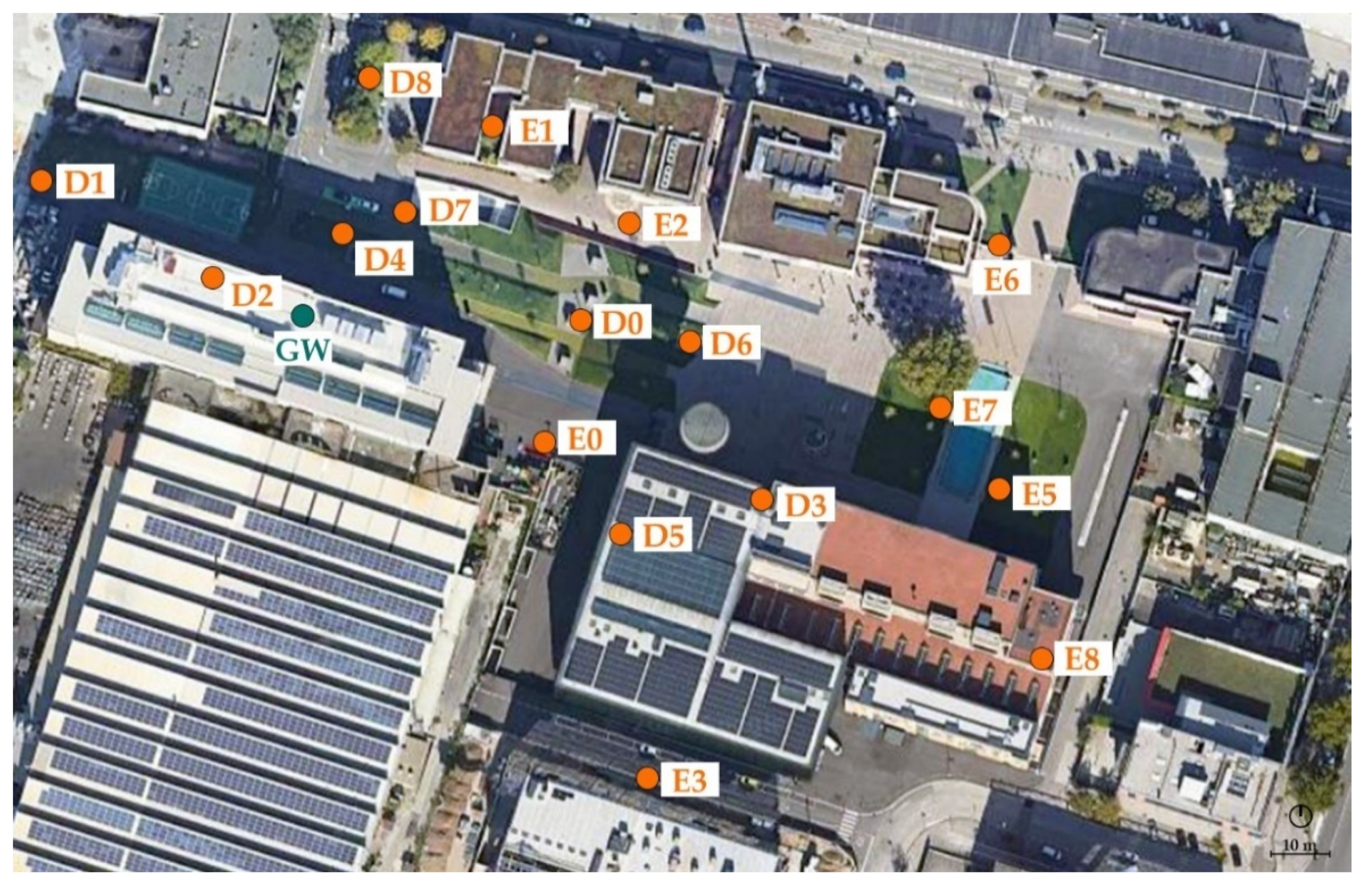
3.2. Deployment of the WSN

The WSN was deployed in the NOI Techpark, a building complex located at the center of the industrial area of Bolzano (highlighted in red in Figure 1). It covers an area of about 0.04 km2. As shown in Figure 3, and described in [43], the measurement point locations were selected to assess the effects of the different surface materials (e.g. asphalt, grass, and natural stone), and of the urban morphology characteristics present in the area. The choice of the positions followed some major siting prescriptions:
  • the sensors should be placed at a height ranging from 1.0 to 2.0 m a.g.l. to be representative of the conditions at pedestrian level [44,45];
  • the sensors should be deployed at a minimum distance of 1.5 m from building walls to avoid the influence of radiation exchanges with the surface in the measurements [30,46] and away from significant heat sources [45,47].
Consequently, all nodes were installed in positions that were far from significant sources of anthropogenic heat; the only exceptions were two sensors that may be influenced by cars parking nearby, (i.e., D8 and E3). The sensor nodes were installed at pedestrian level, with three exceptions: two sensors installed on roofs of buildings having different heights (i.e., D2 and E8), and one in a winter garden located at the second floor of the main building (i.e., D5). The data acquired by these sensors are not used for the characterization of microclimate conditions at pedestrian level. They are, however, representative of areas used for various purposes by the employees of NOI Techpark.

4. Mobile Monitoring Approach

In this section, the components of the mobile microclimate sensing system, namely the hardware prototypes and the EDP’s building blocks that allow the data workflow/visualization/analysis, are presented. The overall approach relies on low-cost hardware and open-source software. Regarding the geo-localization needs for a mobile solution, global navigation satellite system (GNSS) receivers and antennas with carrier phase, code phase, and Doppler measurement capabilities were implanted in the solution to allow for accurate positioning and, eventually, real-time-kinematics (RTK) correction. The receivers were chosen from among low-cost options, and feature a number of channels able to concurrently acquire signals from Navstar, Glonass, and Galileo constellations. The workflow was developed in a cloud-oriented perspective. This design is favorable for performing RTK by exploiting public positioning services as base stations and, therefore, achieving greater geo-localization accuracy [48]. This provides the two-fold benefit of reducing the hardware complexity (i.e., only rover units are needed), and enhancing the operation range of the prototypes (i.e., once the rovers have transferred their raw data to the cloud, they can enter sleep mode without waiting for/downloading the base station correction file to perform RTK correction locally). Instead, an always-on service in the cloud can be automated to publish the dataset of a new field campaign as soon as it has been properly pre-processed and verified.

4.1. Hardware Prototypes

The hardware prototyping was based on a Raspberry Pi (RPi) as the core unit. This is one of the most flexible and supported options that are currently available for low-cost development. The advantages include the large number of connection buses already on-board, the availability of many different expansion modules to provide additional features, and the software environment, which ranges from a light command line interface to a whole operating system, as needed. The main disadvantages are the high power usage and the limited stability/reliability due to the fact that RPi is still a development board.
Coupled with the RPi module 3b+, the following components were present:
  • RCmall SIM800 GSM GPRS expansion shield V2.3;
  • Adafruit PiTFT 3.5” touch screen interface;
  • u-blox C099-F9P board with an ANN-MB00 multi-band GNSS antenna + ground plate;
  • Anker USB power bank 5V–15,000 mAh;
  • Galltec PM15PS humidity/temperature sensor with RS232 signal level converter
  • Apogee SP420 silicon-cell USB pyranometer;
  • Meter Environment solar radiation shield;
  • BOPLA Bocube IP-68 170 × 271 × 90 mm.
An in-depth description of the assembly and characterization of the prototypes’ building blocks is provided in [49]. Similar prototyping can be accomplished by means of a different core unit, for instance, an industrial grade microcontroller [50]. This would enable a more reliable interaction between the system components, in addition to lower power consumption. However, this comes at the cost of a longer development time. For the reasons of clarity, here we report only the prototype’s figures that are relevant for the current case study:
  • RH accuracy ± 1.5% RH;
  • Tair accuracy ± 0.15 °C;
  • positioning accuracy of 0.3 m northing/easting in rover configuration (0.01 m northing/easting positional accuracy in rover configuration when RTK is implemented).
In Figure 4, the two prototypes completed for the testbed are shown in the laboratory (left) and when mounted on city bicycles (right). During the installation, trade-off criteria between encumbrance, handling, and best positioning of the sensors were addressed. In previous work [49], a 2 m high rod attached to the bicycle frame for the GNSS antenna and a gimbal as a mount for the pyranometer was used. In this manner, the perturbation caused by the biker on the satellite signal and the non-horizontal positioning of the pyranometer in motion can be mitigated. Moreover, this is compliant with the certified monitoring stations’ measurements, which typically measure climatic parameters at 2 m a.g.l. (at the level of the average person’s head). However, such arrangements make the bicycle uncomfortable and less convenient. Thus, improving the measurement due to such configurations will be estimated in a follow-up work.

4.2. Workflow and Data Fusion

The data acquisition workflow for the mobile monitoring approach is shown in Figure 5. The leftmost side shows the prototype schematics based on the two development boards previously described in Section 4.1. Each field campaign must be started through the touchscreen interface. This operation triggers the sensors and the GNSS acquisition. The data acquisition rate is preset to 1 Hz to cope with sensors refresh rate and geo-localization accuracy. When the field campaign finishes, the data payload is formatted as two separate files: a .txt file carrying Tair and RH (and solar radiation), and a .ubx file carrying the GPS log data format. The two files are saved locally, and also sent through a 3GPP connection via file transfer protocol (FTP) from the prototype to the EDP back-end. This operation is performed by a shell script running as a service on the Raspberry each time a field campaign is accomplished. In the back-end, a similar method was set up based on a cronjob in order to pre-process the new files as soon as they are received. The pre-processing operations are performed on a Linux virtual machine running the RTK lib suite [51]. First, the GNSS.ubx file is converted into a receiver independent exchange format (RINEX) file by means of convbin. rnx2rtkp can be optionally exploited to achieve a RTK correction when the data from a base station are available. Then, the environmental measurements are aggregated with the GNSS data, thus creating a geo-localized data-frame in which the sensors’ acquisition is also synced with the GNSS time. Before the storage in a PostgreSQL database, the data are augmented with metadata specifying the means of transportation (pedestrian, bicycle, car), the unit id (person name, bicycle number, car plate), and the context (urban, peri-urban, countryside, etc.). All the metadata are preset in the hardware prototypes and can be updated with ease from the touchscreen through a graphical user interface (GUI) specifically developed with Python and Tkinter for this purpose.
Via GeoServer, the spatial data are made available in Web Map Service (WMS). The web graphic information system (GIS) used by the EPD is GeoNode, which allows for a comprehensive visualization and filtering of the acquired dataset both from PCs and mobile devices. Furthermore, for the purpose of the data analysis, dedicated snipped codes can be downloaded from the EPD to consume the data in different processing environments (R-studio, Python, or Java clients). By doing so, the database can be properly queried, as described in Section 5.2.

4.3. Exploratory Field Campaigns

An exploratory field campaign was carried out in May 2021 to validate the effectiveness of the approach for monitoring the diurnal evolution of the microclimate conditions (Tair/RH fields). Data were acquired in three sessions during daytime on weekdays: at morning (i.e., 08:30–10:30), noon (i.e., 12:00–14:00), and afternoon (i.e., 16:00–18:00). The measurements were carried out in 8 days, chosen for the stationary weather conditions (i.e., clear sky and absence of wind). The selected pathway had a length of 9 km, starting and ending at NOI Techpark, crossed the city center, and reached the northern part of the city. It was specifically designed to monitor areas of Bolzano characterized by different land use, urban morphology, and human activities (Figure 6). Because the field campaign was carried out for test purposes, the selected path represents a trade-off between spatial extension, representativeness of measurement points, and time required for covering the entire pathway. A more extensive data collection, both in terms of spatial coverage and time, would have required resources not available during the pandemic of 2020–2021. Future campaigns will be more structured, and will include other districts, such as high-density residential areas, to enhance the representativeness of the collected data and extend the analysis of local climate conditions to the entire city.
Along the planned urban path, six fixed stops were selected in order to provide a dense acquisition of measurements in points representative of different urban areas (e.g., industrial, residential, green areas). Specifically, 5- to 10-min stops were performed in six points, highlighted in Figure 6. This strategy ensured overlapping acquisition points at each step of the field campaign. Indeed, although the geo-localization of the mobile prototypes is highly accurate, the transition between floating and fixed positional solutions may take some time, especially in urban canyons. Until the solutions are fixed, the correct aggregation of the environmental measurements to the real coordinates in which they are taken is prevented.
The six points were chosen as being representative of specific characteristics of the different areas of the city crossed by the pathway, including locations in built-up areas close to roads with high traffic levels (P1 and P2) and in proximity to public green areas within the city center (P3 and P4); positions close to the Talvera river (P5); and positions in the outskirts of the city next to open fields (P6). Furthermore, stops were also performed in proximity to sensors of the fixed WSN in the NOI Techpark.
Data collected from a fixed high-resolution weather station installed on the roof of the NOI Techpark (location shown in Figure 6) were used for defining the climatic boundary conditions of each monitoring campaign. The weather station was an ATMOS 41 by Meter Group [52], and the measurement time step was set to 30 min.

5. Preliminary Results and Open Issues

In the following sections, preliminary experimental acquisitions in conjunction with considerations in regards to long-lasting adoption are discussed for both the fixed (Section 3) and the mobile (Section 4) monitoring approaches.

5.1. Fixed Monitoring Approach

For the purpose of this work, the two summer months from 15 July to 15 September 2020 were surveyed and analyzed, with a focus on the distribution of the microclimate parameters in relation to the urban morphology of the area and the ground cover.

5.1.1. WSN Reliability

During the two months of operation, some issues occurred, both related to data transmission and to failures of hardware components. Regarding the data transmission, the percentage of data lost was close to 0% for most of the nodes, with the exception of three. D0 and E6 showed a packet loss ratio of around 10% to 15% of the total amount of expected data. Moreover, that of E1 exceeded 50%, with more than 410 h incurring a fault in total. With regard to the functioning of hardware components, sensors’ readout saturation contributed to less than 1% of the measurements in the majority of the sensors. In four sensor nodes, this threshold was exceeded with saturations up to 4.8% of the measurements, requiring the replacement of the Tair/RH sensing element during the campaign. Several sensors required other maintenance interventions during the two months of operation, as show in Figure 7. A manual reboot was executed on 10 sensors for a total of 30 times. The battery was changed in six sensors, the microcontroller in one, and three sensors required testing in the laboratory. In addition to the laboratory testing, the other maintenance interventions were communicated to the EDP by the sensor nodes themselves, allowing for the following plot on a real-time dashboard.

5.1.2. Field Campaign in Summer Conditions

The analysis of the data collected during the summer field campaign was aimed at understanding whether the WSN is suitable to investigate the correlation between urban morphology and microclimate conditions. Hence, the following section discusses the influence of parameters such as sky-view factor, aspect ratio, and the presence of vegetation and typology of ground cover on Tair and RH (Figure 3 and Table 1). Because the results discussed are preliminary, and more extensive field campaigns will be carried out in the future, the summer distribution of Tair and RH in the NOI Techpark was analyzed by focusing on the daily trend of hourly averaged (avg) values (Figure 8).
During daytime, the highest values were recorded between 14:00 and 16:00 in all the acquisition points. The sensor node D2, located on the concrete roof of a building in an un-shaded position (SVF = 0.950), recorded the highest air temperature (avg Tair = 32.7 °C at 14:00). Nine other sensor nodes (i.e., D0, D1, D6, D7, E0, E2, E6, E8)—all characterized by SVF values higher than 0.500 and locations with a high number of hours with direct sunlight—presented avg Tair ≥ 30.0 °C during daytime. The higher values were recorded in points characterized by artificial surfaces, i.e., granite in E0 and porphyry in E2, showing the relevant influence of ground cover materials in increasing local temperatures. During daytime, the nodes characterized by low SVF and, consequently, low levels of direct solar irradiation (i.e., E1, E3, and D3) showed lower Tair. The influence of the sky-view factor is also evident at night-time. Indeed, low SVF implies a reduced net longwave loss, especially at night, when the heat stored by the building materials during daytime could not be re-radiated back to the atmosphere. This phenomenon contributes to increased air temperatures in D5 and D3.
The cooling effect due to evapotranspiration is noticeable in points located in proximity to vegetation. This is particularly evident in nodes E5 and E7, which are deployed in the green area close to the water body, where both grass and trees are present. The nodes are also characterized by the lowest temperatures during night-time. On the contrary, the cooling effect is limited in the green area located over the underground parking area (i.e., sensor nodes D4, D7, D0 and D6), due to the limited depth of soil substrate and the presence of a small number of trees providing very limited shadow. The influence of evapotranspiration is also confirmed by the distribution of hourly relative humidity values (Table 1). Indeed, higher RH percentages were recorded in points located in proximity to vegetated areas (e.g., E5 and E7), especially during night-time.

5.1.3. Evaluation of UHI Intensity

The comparison of the air temperature values recorded in the area of NOI Techpark (solid lines in Figure 8) with the values measured by the South Tyrol weather service stations (dashed lines in Figure 8) provides an insight into the extent of summer overheating in the monitored area. Compared to the UWS, the NOI Techpark presents higher Tair during daytime, with an average delta of +1.8 °C, whereas the temperatures are almost the same or slightly colder (up to −1.0 °C) during night-time. The hottest daytime conditions are explained by the higher share of sealed surfaces and higher anthropogenic heat release in the Bolzano South industrial area compared to the area of the hospital and its surroundings, which are mainly vineyards.
The presence of UHI in Bolzano South was confirmed by comparing the air temperature values at NOI Techpark with those at the RWS location. In the two analyzed summer months, the average daytime UHI was around 2.7 °C. The differences in air temperatures started to increase from 06:00, reached a maximum in the late morning, with ΔTair (urban,rural) = 3.6 °C, and then decreased until 20:00, when the delta was almost negligible. During night-time, ΔTair (urban,rural) started to intensify again from 21:00 and reached its maximum at sunrise, around 06:00 (i.e., ΔTair (urban,rural) = 1.8 °C). However, night-time UHI intensity was lower than that of daytime, with an average value around 1.1 °C. This latter result highlights the relevance of anthropogenic heat sources in contributing to the temperature increase, as the heat release mainly happens during the day, related to traffic conditions, and offices and industries in operation.

5.1.4. Limits of the Fixed Monitoring Approach

In addition to the reliability issues already discussed in Section 5.1.1, the fixed monitoring campaign at NOI Techpark presents two main limitations, which will be addressed in the future developments of the WSN. First, there is a lack of reference weather stations located in the Bolzano South area for a further validation of the WSN’s data and for a proper evaluation of UHI intensity. Second, the calibration of the low-cost sensors should consider the potential overheating related to a non-optimal ventilation within the low-cost radiation shields. This is a complex effect to be simulated in a supervised environment (i.e., a microclimatic chamber). For this reason, the comparison with high-accuracy reference instruments should be carried out directly in the field during real-operation conditions. Then, the acquired data can be adjusted by gain and offset values, calculated from these comparative measurements, as suggested in [51].

5.2. Mobile Monitoring Approach

5.2.1. Exploratory Field Campaign

Overall, the results of the exploratory campaign showed that the mobile monitoring approach highlights the intra-urban variation of the measured microclimate variables (i.e., Tair, RH, and solar radiation), as represented in Figure 9 for Tair. Indeed, for each variable, localized hot-spots can be identified. As an example, the highest values of Tair were recorded in Bolzano South, and in proximity to roads with elevated traffic levels. On the contrary, the cooling effect of vegetation and water is evident in the measurements alongside the Talvera river, where values up to 1.0 °C cooler were recorded during the monitoring campaigns at noon and afternoon.
As the main purpose of the data collections was to test the suitability of the sensors for the mobile monitoring of microclimate parameters and for the evaluation of UHI intensity, the following discussion is focused on Tair data acquired during the field campaign of 4 May 2021. In the plot in Figure 9, the entire mobile monitoring dataset is filtered to show only the acquisitions performed at the six predefined points. This is possible through separated queries with a 1 m radius centered at the geographical coordinates of the predefined points. This filtering provides a set of temperature data that can be clustered/averaged by hour of the day, and day, to obtain a scatter plot. From the analysis of the three campaigns (i.e., morning, noon, and afternoon) of the selected day, shown in the inset, some main considerations can be inferred:
  • the data correctly represent the increase in air temperature during daytime;
  • the temperature is higher in dense urban areas close to major roads, both in the industrial area (Points 1 and 2) and in the city center (Point 3); it decreases in the open green areas close to the Talvera river (Points 4 and 5); and it drops in the northern area of the city, where the building density is lower (Point 6);
  • the measurements also confirmed the presence of a UHI in Bolzano South. Indeed, Tair at points located in the industrial area is up to 1.5 °C higher than that in the other districts of the city. This trend is more evident at noon and during the afternoon, when higher temperatures are reached.

5.2.2. Limits of the Mobile Monitoring Approach

Considering that the hardware prototypes were mounted on forms of transport (i.e., bicycles) that may experience intense vibrations while moving, the devices showed a high working reliability. Indeed, during more than 30 urban surveys, only one data acquisition stopped due to a hard impact that caused some wires to become unplugged.
One of the main issues of the proposed approach is the high power demand of the core unit. Indeed, the coupling of the Rpi with the F9P board, combined with the high-frequency acquisition of the environmental parameters, requires daily charging cycles. Another factor that limits such an approach, per se, is the need for the human intervention to start each field campaign. Although the touch screen interface is highly user-friendly, minimum training should be provided to the biker in advance. Moreover, the risk of forgetting to start the device when the bicycle is used to perform another task, in addition to the urban surveying, is significant. This can be prevented by considering an always-on acquisition. However, this methodology could be implemented only on cars, e-bikes, or e-scooters, but at the cost of a deep intervention into several of the vehicle’s components. Finally, but also importantly, the lack of geo-spatial overlap between the survey paths can be a major issue, especially when we foresee that the field campaigns may be undertaken by inexperienced persons.

6. Conclusions and Future Perspectives

The current work reports the development and testing of two environmental monitoring networks, one fixed and one mobile, based on low-cost hardware and open-source software, aimed at characterizing the microclimate conditions and their spatial variations in urban areas. A critical comparison between the two approaches was carried out, highlighting the favorable and the limiting features in both cases. The sensor networks proved their suitability for the monitoring of micro-meteorological variables with high spatial resolution at different scales: a neighborhood scale in the case of fixed sensors, up to a city scale in the case of mobile sensors. Furthermore, the analysis of the preliminary datasets acquired, even if limited in terms of the time span, demonstrated the soundness of the proposed methods. Indeed, the spatial resolution of the data allows representing the variation of microclimate conditions among different areas within Bolzano, in addition to the influence of the unique conditions of each location, such as the distribution and density of the buildings, the surfaces materials, and the presence of vegetation. This offers several opportunities for the analysis of environmental phenomena in urban areas, such as the UHI, and for supporting the definition of climate change mitigation, adaptation, and resilience policies at the city level. Furthermore, the acquired dataset may be combined with numerical simulations. Indeed, real data can provide an improved basis for the validation of computational approaches. Moreover, numerical models calibrated with distributed monitoring data offer the opportunity to expand the analysis domain at broader scales with high spatial-temporal resolution.
In addition, the combination of the proposed approaches may represent a useful tool for monitoring the impacts of mitigation strategies in cities, as in the case of nature-based solutions. As an example, this would allow quantifying the expected beneficial effects of greening with regard to the reduction in peak temperatures and the improvement in thermal comfort.
Finally, we foresee significant opportunity for the pervasive spread of both of the studied approaches once the issues encountered during the validation phase are properly addressed. Indeed, no serious technology/methodology barriers have been identified thus far, whereas many benefits have been demonstrated. These include an unprecedented monitoring granularity regarding fixed networks of low-cost sensors (meshing down to tens of meters). On the contrary, the exploitation of mobile sensor nodes allows expanding the surveying domain while dramatically lowering the hardware and maintenance costs. Moreover, by relying on an open-source and FAIR-oriented data platform, the approaches can be further developed to provide cross-domain services, such as the estimation of the statistical correlations between the urban surface-usage/morphology and local microclimate conditions.

Author Contributions

Conceptualization, S.C. and S.T.; methodology, S.C.; software, S.T.; validation, S.C. and S.T.; formal analysis, S.C.; investigation, S.C. and S.T.; resources, S.T.; data curation, S.C. and S.T.; writing—original draft preparation, S.C. and S.T.; writing—review and editing, S.C. and S.T.; visualization, S.C. and S.T.; supervision, S.T.; project administration, S.T. All authors have read and agreed to the published version of the manuscript.

Funding

The research leading to these results has received funding from the European Regional Development Fund, Operational Programme Investment for growth and jobs ERDF 2014–2020 under Project number ERDF1094, Data Platform and Sensing Technology for Environmental Sensing LAB–DPS4ESLAB, and from the European Union’s Seventh Programme for research, technological development and demonstration under grant agreement No. 609019. The European Union is not liable for any use that may be made of the information contained in this document.

Data Availability Statement

The data presented in this study are openly available in [https://maps.eurac.edu/layers/dps4eslab-urban:geonode:dps_urban, accessed on 1 December 2021] at [https://0-doi-org.brum.beds.ac.uk/10.48784/s63z-6330, accessed on 1 December 2021].

Acknowledgments

The authors acknowledge Roberto Monsorno, leader of the DPS4ESLAB project and Daniele Vettorato, leader of Urban and Regional Energy System group, for supporting the startup of the research activities; Antonio Novelli and Lavinia Laiti for the preliminary discussions about the study case of distributed urban microclimate monitoring in Bolzano; and Simone Tritini and Andrea Vianello for the technical support related to the Environmental Data Platform of Eurac Research.

Conflicts of Interest

The authors declare no conflict of interest. The funders had no role in the design of the study; in the collection, analyses, or interpretation of data; in the writing of the manuscript, or in the decision to publish the results.

References

  1. Hoornweg, D.; Sugar, L.; Gómez, C.L.T. Cities and greenhouse gas emissions: Moving forward. Environ. Urban. 2011, 23, 207–227. [Google Scholar] [CrossRef]
  2. Baklanov, A.; Grimmond, S.; Carlson, D.; Terblanche, D.; Tang, X.; Bouchet, V.; Lee, B.; Langendijk, G.; Kolli, R.; Hovsepyan, A. From urban meteorology, climate and environment research to integrated city services. Urban Clim. 2018, 23, 330–341. [Google Scholar] [CrossRef]
  3. Revi, A.; Satterthwaite, D.; Aragón-Durand, F.; Corfee-Morlot, J.; Pelling, M.; Roberts, D.C.; Solecki, W.; Kiunsi, R.B.R. Urban Areas in Climate Change 2014: Impacts, Adaptation, and Vulnerability. Part A: Global and Sectoral Aspects. Contribution of Working Group II to the Fifth Assessment Report of the Intergovernmental Panel on Climate Change; Cambridge University Press: Cambridge, UK, 2014; pp. 535–612. [Google Scholar]
  4. Garcia, D.J.; You, F. The water-energy-food nexus and process systems engineering: A new focus. Comput. Chem. Eng. 2016, 91, 49–67. [Google Scholar] [CrossRef]
  5. Oke, T.R.; Mills, G.; Christen, A.; Voogt, J.A. Urban Climates; Cambridge University Press: Cambridge, UK, 2017. [Google Scholar]
  6. Lemonsu, A.; Viguié, V.; Daniel, M.; Masson, V. Vulnerability to heat waves: Impact of urban expansion scenarios on urban heat island and heat stress in Paris (France). Urban Clim. 2015, 14, 586–605. [Google Scholar] [CrossRef]
  7. Bozonnet, E.; Musy, M.; Calmet, I.; Rodriguez, F. Modeling methods to assess urban fluxes and heat island mitigation measures from street to city scale. Int. J. Low-Carbon Technol. 2013, 10, 62–77. [Google Scholar] [CrossRef] [Green Version]
  8. Erell, E. The Application of Urban Climate Research in the Design of Cities. Adv. Build. Energy Res. 2008, 2, 95–121. [Google Scholar] [CrossRef]
  9. Taha, H. Urban climates and heat islands: Albedo, evapotranspiration, and anthropogenic heat. Energy Build. 1997, 25, 99–103. [Google Scholar] [CrossRef] [Green Version]
  10. Ulpiani, G. On the linkage between urban heat island and urban pollution island: Three-decade literature review towards a conceptual framework. Sci. Total Environ. 2020, 751, 141727. [Google Scholar] [CrossRef]
  11. Salata, F.; Golasi, I.; Petitti, D.; Vollaro, E.D.L.; Coppi, M.; Vollaro, A.D.L. Relating microclimate, human thermal comfort and health during heat waves: An analysis of heat island mitigation strategies through a case study in an urban outdoor environment. Sustain. Cities Soc. 2017, 30, 79–96. [Google Scholar] [CrossRef]
  12. Heaviside, C.; Vardoulakis, S.; Cai, X.-M. Attribution of mortality to the urban heat island during heatwaves in the West Midlands, UK. Environ. Health 2016, 15, 49–59. [Google Scholar] [CrossRef] [Green Version]
  13. Paravantis, J.; Santamouris, M.; Cartalis, C.; Efthymiou, C.; Kontoulis, N. Mortality Associated with High Ambient Temperatures, Heatwaves, and the Urban Heat Island in Athens, Greece. Sustainability 2017, 9, 606. [Google Scholar] [CrossRef] [Green Version]
  14. Dang, T.N.; Van, D.Q.; Kusaka, H.; Seposo, X.T.; Honda, Y. Green Space and Deaths Attributable to the Urban Heat Island Effect in Ho Chi Minh City. Am. J. Public Health 2018, 108, S137–S143. [Google Scholar] [CrossRef] [PubMed] [Green Version]
  15. Santamouris, M.; Papanikolaou, N.; Livada, I.; Koronaki, I.; Georgakis, C.; Argiriou, A.; Assimakopoulos, D. On the impact of urban climate on the energy consumption of buildings. Sol. Energy 2001, 70, 201–216. [Google Scholar] [CrossRef]
  16. Li, X.; Zhou, Y.; Yu, S.; Jia, G.; Li, H.; Li, W. Urban heat island impacts on building energy consumption: A review of approaches and findings. Energy 2019, 174, 407–419. [Google Scholar] [CrossRef]
  17. Roxon, J.; Ulm, F.-J.; Pellenq, R.-M. Urban heat island impact on state residential energy cost and CO2 emissions in the United States. Urban Clim. 2019, 31, 100546. [Google Scholar] [CrossRef]
  18. Sanchez-Guevara, C.; Peiró, M.N.; Taylor, J.; Mavrogianni, A.; González, J.N. Assessing population vulnerability towards summer energy poverty: Case studies of Madrid and London. Energy Build. 2019, 190, 132–143. [Google Scholar] [CrossRef] [Green Version]
  19. Tsilini, V.; Papantoniou, S.; Kolokotsa, D.; Maria, E.-A. Urban gardens as a solution to energy poverty and urban heat island. Sustain. Cities Soc. 2015, 14, 323–333. [Google Scholar] [CrossRef]
  20. Pisello, A.L.; Saliari, M.; Vasilakopoulou, K.; Haddad, S.; Santamouris, M. Facing the urban overheating: Recent developments. Mitigation potential and sensitivity of the main technologies. Wiley Interdiscip. Rev. Energy Environ. 2018, 7. [Google Scholar] [CrossRef]
  21. Shooshtarian, S.; Rajagopalan, P.; Sagoo, A. A comprehensive review of thermal adaptive strategies in outdoor spaces. Sustain. Cities Soc. 2018, 41, 647–665. [Google Scholar] [CrossRef]
  22. Kousis, I.; Pigliautile, I.; Pisello, A.L. Intra-urban microclimate investigation in urban heat island through a novel mobile monitoring system. Sci. Rep. 2021, 11, 1–17. [Google Scholar] [CrossRef]
  23. Masson, V.; Heldens, W.; Bocher, E.; Bonhomme, M.; Bucher, B.; Burmeister, C.; de Munck, C.; Esch, T.; Hidalgo, J.; Kanani-Sühring, F.; et al. City-descriptive input data for urban climate models: Model requirements, data sources and challenges. Urban Clim. 2019, 31, 100536. [Google Scholar] [CrossRef]
  24. Shaker, R.R.; Altman, Y.; Deng, C.; Vaz, E.; Forsythe, K. Investigating urban heat island through spatial analysis of New York City streetscapes. J. Clean. Prod. 2019, 233, 972–992. [Google Scholar] [CrossRef]
  25. Tsoka, S.; Tsikaloudaki, K.; Theodosiou, T.; Bikas, D. Urban Warming and Cities’ Microclimates: Investigation Methods and Mitigation Strategies—A Review. Energies 2020, 13, 1414. [Google Scholar] [CrossRef] [Green Version]
  26. Amirtham, L.R. Urbanization and its impact on Urban Heat Island Intensity in Chennai Metropolitan Area, India. Indian J. Sci. Technol. 2016, 9. [Google Scholar] [CrossRef] [Green Version]
  27. de Jesus, M.P.; Lourenco, J.M.; Arce, R.M.; Macias, M. Green façades and in situ measurements of outdoor building thermal behaviour. Build. Environ. 2017, 119, 11–19. [Google Scholar] [CrossRef] [Green Version]
  28. Chen, Y.C.; Liao, Y.-J.; Yao, C.-K.; Honjo, T.; Wang, C.-K.; Lin, T.-P. The application of a high-density street-level air temperature observation network (HiSAN): The relationship between air temperature, urban development, and geographic features. Sci. Total Environ. 2019, 685, 710–722. [Google Scholar] [CrossRef] [PubMed]
  29. Chokhachian, A.; Lau, K.K.-L.; Perini, K.; Auer, T. Sensing transient outdoor comfort: A georeferenced method to monitor and map microclimate. J. Build. Eng. 2018, 20, 94–104. [Google Scholar] [CrossRef]
  30. Busato, F.; Lazzarin, R.; Noro, M. Three years of study of the Urban Heat Island in Padua: Experimental results. Sustain. Cities Soc. 2014, 10, 251–258. [Google Scholar] [CrossRef]
  31. Georgakis, C.; Santamouris, M. Determination of the Surface and Canopy Urban Heat Island in Athens Central Zone Using Advanced Monitoring. Climate 2017, 5, 97. [Google Scholar] [CrossRef] [Green Version]
  32. MIT Senseable City Lab. City Scanner 2021. Available online: http://senseable.mit.edu/cityscanner/app/#15/42.3643/-71.1008 (accessed on 1 December 2021).
  33. Yang, J.; Bou-Zeid, E. Designing sensor networks to resolve spatio-temporal urban temperature variations: Fixed, mobile or hybrid? Environ. Res. Lett. 2019, 14, 074022. [Google Scholar] [CrossRef]
  34. Wilkinson, M.D.; Dumontier, M.; Aalbersberg, I.J.; Appleton, G.; Axton, M.; Baak, A.; Blomberg, N.; Boiten, J.-W.; da Silva Santos, L.B.; Bourne, P.E.; et al. The FAIR Guiding Principles for scientific data management and stewardship. Sci. Data 2016, 3, 160018. [Google Scholar] [CrossRef] [PubMed] [Green Version]
  35. Kottek, M.; Grieser, J.; Beck, C.; Rudolf, B.; Rubel, F. World Map of the Köppen-Geiger climate classification updated. Meteorol. Z. 2006, 15, 259–263. [Google Scholar] [CrossRef]
  36. Papathoma-Köhle, M.; Ulbrich, T.; Keiler, M.; Pedoth, L.; Totschnig, R.; Glade, T.; Schneiderbauer, S.; Eidswig, U. Vulnerability to Heat Waves, Floods, and Landslides in Mountainous Terrain. In Assessment of Vulnerability to Natural Hazards. A European Perspective; Elsevier: Amsterdam, The Netherlands, 2014; pp. 179–201. [Google Scholar] [CrossRef]
  37. Weather South Tyrol. Weather Station Branzoll 2020. Available online: http://weather.provinz.bz.it/weather-stations-valley.asp?stat_stid=1220 (accessed on 1 December 2021).
  38. LoRaWAN@NOI Web Portal 2020. Available online: https://lorawan.beacon.bz.it/ (accessed on 1 December 2021).
  39. LoraWAN Gateway Setup n.d. Available online: https://gitlab.inf.unibz.it/CSS-DEV/projects/lorawan-gateway-setup (accessed on 1 December 2021).
  40. Tondini, S.; Tritini, S.; Amatori, M.; Croce, S.; Seppi, S.; Monsorno, R. LoRa-based Wireless Sensor Networks for Urban Scenarios Using an Open-source Approach. Sens. Trasducers 2019, 238, 64–71. [Google Scholar]
  41. Croce, S.; Tondini, S. Urban Microclimate Monitoring and Modeling through an Open-Source Distributed Network of Wireless Low-Cost Sensors and Numerical Simulations. In Proceedings of the 7th International Electronic Conference on Sensors and Applications, Basel, Switzerland, 15–30 November 2020; Volume 2, p. 18. [Google Scholar] [CrossRef]
  42. Acero, J.A.; Herranz-Pascual, K. A comparison of thermal comfort conditions in four urban spaces by means of measurements and modelling techniques. Build. Environ. 2015, 93, 245–257. [Google Scholar] [CrossRef]
  43. Sharmin, T.; Steemers, K.; Matzarakis, A. Analysis of microclimatic diversity and outdoor thermal comfort perceptions in the tropical megacity Dhaka, Bangladesh. Build. Environ. 2015, 94, 734–750. [Google Scholar] [CrossRef]
  44. Dimoudi, A.; Kantzioura, A.; Zoras, S.; Pallas, C.; Kosmopoulos, P. Investigation of urban microclimate parameters in an urban center. Energy Build. 2013, 64, 1–9. [Google Scholar] [CrossRef]
  45. Tong, S.; Wong, N.H.; Jusuf, S.K.; Tan, C.L.; Wong, H.F.; Ignatius, M.; Tan, E. Study on correlation between air temperature and urban morphology parameters in built environment in northern China. Build. Environ. 2018, 127, 239–249. [Google Scholar] [CrossRef]
  46. Teunissen, P.; Khodabandeh, A. Review and principles of PPP-RTK methods. J. Geodesy 2015, 89, 217–240. [Google Scholar] [CrossRef]
  47. Tondini, S.; Hasanabadi, F.; Monsorno, R.; Novelli, A. Toward near real-time kinematics differential correction: In view of geo-metrically augmented sensor data for mobile microclimate monitoring. Eng. Proc. 2020, 2, 61. [Google Scholar] [CrossRef]
  48. Allied Market Research. Microcontroller Market by Product Type and Application: Global Opportunity Analysis and Indus-Try Forecast, 2020–2027; Allied Market Research: Portland, OR, USA, 2020. [Google Scholar]
  49. RTKLIB: An Open Source Program Package for GNSS Positioning n.d. Available online: http://www.rtklib.com/ (accessed on 1 December 2021).
  50. Meter Environment. ATMOS 41 All-in-One Weather Station 2018. Available online: https://www.metergroup.com/environment/products/atmos-41-weather-station/ (accessed on 1 December 2021).
  51. Grykałowska, A.; Kowal, A.; Szmyrka-Grzebyk, A. The basics of calibration procedure and estimation of uncertainty budget for meteorological temperature sensors. Meteorol. Appl. 2015, 22, 867–872. [Google Scholar] [CrossRef]
  52. Chapman, L.; Muller, C.L.; Young, D.T.; Warren, E.; Grimmond, S.; Cai, X.-M.; Ferranti, E. The Birmingham Urban Climate Laboratory: An Open Meteorological Test Bed and Challenges of the Smart City. Bull. Am. Meteorol. Soc. 2015, 96, 1545–1560. [Google Scholar] [CrossRef]
Figure 2. (a) Picture of one sensor node; (b) building block schematics of the sensor-node; (c) LoRaWAN gateway that forwards the data packets from the sensor nodes to the EDP; (d) EDP components that allow the proper management of the network.
Smartcities 05 00004 g002
Figure 3. WSN deployment within the NOI Techpark area (Bolzano South): location of sensor nodes (orange) and gateway (GW, blue). Aerial image source: Google Maps.
Smartcities 05 00004 g003
Figure 4. (left) Two completed prototypes housed in an IP-68 case. The touch screen interface, the GNSS double frequency antenna, and the T/RH sensor hosted in a solar radiation shield can be seen in the picture. (right) One prototype as it was installed on a Eurac Research bicycle. The pyranometers are mounted on the outermost support of the luggage carrier.
Smartcities 05 00004 g004
Figure 5. Automatized data acquisition workflow exploited in the mobile monitoring approach. The schematic is split into its three main components: the hardware prototype on the left, the EDP front-end in the middle, and the EPD back-end on the right. The EDP front-end is the access point for the end-users who are interested in the visualization/processing of the data collected during the field campaigns.
Smartcities 05 00004 g005
Figure 6. Selected pathway for the mobile monitoring campaigns. Aerial image source: [39].
Smartcities 05 00004 g006
Figure 7. Maintenance interventions on the WSN sensor nodes in the period from 15 July to 15 September 2020.
Smartcities 05 00004 g007
Figure 8. Hourly averaged air temperature recorded by the sensor nodes (solid) and by the South Tyrol Province urban (UWS) and rural (RWS) weather station (dashed) in the period 15 July–15 September 2020.
Smartcities 05 00004 g008
Figure 9. Filtering of the Tair data acquired by the mobile monitoring prototypes at relevant points distributed along the city of Bolzano. The time series obtained are shown in the plot on the right. An inset shows the temperature daily trends at the specific acquisition points.
Smartcities 05 00004 g009
Table 1. Morphological characteristics and hourly averaged air temperature and relative humidity values measured by the sensor nodes in coldest (i.e., 06:00) and hottest (i.e., 15:00) conditions from 15 July to 15 September 2020.
SensorUrban MorphologyTair [°C] *RH [%] *
Ground CoverVegetationSVFH/W06:0015:0006:0015:00
D0Wooden planks-0.6880.5417.3429.5484.2144.37
D1Grass/asphalt-0.6311.1917.7630.2781.0041.91
D2Concrete-0.950-18.6832.5783.0339.32
D3Granite-0.000-19.9726.1673.6552.40
D4GrassSmall single tree0.5670.7317.8227.4287.7353.19
D5Porphyry/glass-0.254-20.5529.9267.8739.19
D6Grass/stone-0.6800.2117.7230.6289.1744.97
D7Grass/asphaltSmall single tree0.6260.7317.7930.1488.1347.10
D8GrassTrees and bushes0.5850.2318.3829.8586.0648.33
E0Granite-0.5350.5418.4130.5888.4047.57
E1GrassSmall trees0.1701.4518.9427.9076.3544.19
E2PorphyrySmall single tree0.5330.7318.1431.1586.5944.06
E3Asphalt-0.3030.9518.4128.9480.2943.80
E5Grass/gravelSmall trees0.6040.5717.7629.0583.6645.42
E6Granite-0.5690.3018.3429.8593.4849.52
E7Grass/gravelTrees0.5500.5717.4529.2994.6049.61
E8Red gravel-0.760-18.1530.1388.0743.61
* Although the sensors have an accuracy of ±0.5 °C on Tair and ±4.0% on RH, we report the values with 4 significant digits as given during the sensor read-out.
Publisher’s Note: MDPI stays neutral with regard to jurisdictional claims in published maps and institutional affiliations.

