Transformation of Test Data for the Specification of a Viscoelastic Marlow Model

Abstract

The combination of hyperelastic material models with viscoelasticity allows researchers to model the strain-rate-dependent large-strain response of elastomers. Model parameters can be identified using a uniaxial tensile test at a single strain rate and a relaxation test. They enable the prediction of the stress–strain behavior at different strain rates and other loadings like compression or shear. The Marlow model differs from most hyperelastic models by the concept not to use a small number of model parameters but a scalar function to define the mechanical properties. It can be defined conveniently by providing the stress–strain curve of a tensile test without need for parameter optimization. The uniaxial response of the model reproduces this curve exactly. The coupling of the Marlow model and viscoelasticity is an approach to create a strain-rate-dependent hyperelastic model which has good accuracy and is convenient to use. Unfortunately, in this combination, the Marlow model requires to specify the stress–strain curve for the instantaneous material response, while experimental data can be obtained only at finite strain rates. In this paper, a transformation of the finite strain rate data to the instantaneous material response is derived and numerically verified. Its implementation enables us to specify hyperelastic materials considering strain-rate dependence easily.

1. Introduction

1.1. Hyperelasticity and Marlow Model

Hyperelastic material models describe the nonlinear elastic behavior by formulating the strain energy density as a function of the deformation state. This elastic potential is expressed as a function of either the strain invariants (${\overline{I}}_1,{\overline{I}}_2,J$) or the principal stretches (${\lambda }_1,{\lambda }_2,{\lambda }_3$). Review articles comparing different hyperelastic models can be found in [1,2,3,4,5].

Most phenomenological hyperelastic models assume a specific function as elastic potential with a couple of model parameters which have to be fitted to the experimental results. Marlow’s model [6] is an exception, since it uses scalar functions instead of scalar parameters to define the material behavior. The model assumes that the strain energy density is independent of the second deviatoric strain invariant and can be decomposed into a deviatoric and a volumetric part:

$$\begin{array}{c}U({\overline{I}}_1,{\overline{I}}_2,J)=U_{dev}\left({\overline{I}}_1\right)+U_{vol}\left(J\right)\end{array}$$

(1)

using

$$\begin{array}{c}\hfill J={\lambda }_1{\lambda }_2{\lambda }_3,{\overline{I}}_1={\overline{\lambda }}_1^2+{\overline{\lambda }}_2^2+{\overline{\lambda }}_3^2,{\overline{I}}_2={\overline{\lambda }}_1^{-2}+{\overline{\lambda }}_2^{-2}+{\overline{\lambda }}_3^{-2},{\overline{\lambda }}_i=J^{-1/3}{\lambda }_i.\end{array}$$

(2)

The volumetric part is only required if the model shall account for compressibility. This assumption (1) is shared by several other models, e.g., the neo-Hookean model, the model of Arruda and Boyce [7], and Yeoh’s model [8]. While the other models postulate specific functions $U_{dev}$ and $U_{vol}$, Marlow pointed out that such a specific assumption is not necessary to be able to adjust the model to test data of a specific material.

In case of an incompressible model, the elastic potential in (1) is defined by a single scalar function $U_{dev}$. Obviously, this function is uniquely determined by the stress–strain response measured in a single test, e.g., a uniaxial tensile test, and can be obtained by some kind of integration. Similarly, the deviatoric part $U_{vol}$ of the potential of a compressible model can be derived from a stress–strain curve of hydrostatic compression tests. Once $U_{vol}$ has been determined, $U_{dev}$ can be obtained from the data of one additional test. This approach enables a very user-friendly implementation of the Marlow model in finite element software. The user simply provides two stress–strain curves in tabular form: the test data of a uniaxial, biaxial, or planar test; and for compressible models, additionally, the test data of a volumetric test. The model constructed from the data reproduces exactly the two specified test curves. This is different from fits of other models, which usually leave a certain gap between model and test data. The extrapolation of the Marlow model to other load cases is based on assumption (1).

Similar to other models neglecting the dependence of the strain energy density on the second invariant ${\overline{I}}_2$, the Marlow model allows an unambiguous identification of its deviatoric part based on a single type of experiment. It should be noted that this does not necessarily imply that the model will make correct predictions under different kinds of loading. In general, it is recommended to use different kinds of tests in the parameter identification for hyperelastic models [1]. In practical application of the models, it is often desirable to reduce the cost of required experiments even if this reduces the accuracy of predictions. Therefore, the Marlow model has gained some popularity.

1.2. Combination of Hyperelasticity and Viscoelasticity

Viscoelastic models allow to describe relaxation and strain-rate-dependent elastic properties. If we consider a shear deformation, an integral formulation of linear small strain viscoelasticity is given by

$$\tau \left(t\right)={\int }_0^t{G}_R(t-t^{\prime })\frac{d\gamma \left(t^{\prime }\right)}{dt}d{t}^{\prime },$$

(3)

where $\tau$ denotes the shear stress, $\gamma$ the shear strain, and $G_R\left(t\right)$ the relaxation function. This can be expressed using the instantaneous shear modulus $G_0$ and a relative relaxation function $g_R\left(t\right)$ by

$$\tau \left(t\right)=G_0{\int }_0^t{g}_R(t-t^{\prime })\frac{d\gamma \left(t^{\prime }\right)}{dt}d{t}^{\prime }.$$

(4)

Usually, the relaxation function is expressed by a Prony series containing N relaxation times ${\tau }_i$ and coefficients $g_i$ as parameters:

$$g_R\left(t\right)=1-\sum _{i=1}^N{g}_i\left(1-e^{-t/{\tau }_i}\right).$$

(5)

This approach can be generalized from small strain elasticity to hyperelasticity by applying the relative relaxation function to the strain energy density:

$$U_R({\overline{I}}_1,{\overline{I}}_2,J,t)=U_0({\overline{I}}_1,{\overline{I}}_2,J)g_R\left(t\right).$$

(6)

In general, it is possible to consider different relaxation functions for the deviatoric part of the potential $U_{dev}$ and the volumetric part $U_{vol}$, but this distinction will not be made in this paper.

The combination of viscoelasticity and hyperelasticity is available in commercial finite element software. The development and application of visco-hyperelastic models is topic of a large number of current publications, e.g., [9,10,11,12]. In a preceding work of the author [13], an attempt was made to identify a visco-hyperelastic model using a minimal number of experiments. Similar to the identification of a Marlow model by a single type of test, only uniaxial loading was employed in the parameter identification of the deviatoric part of the model. First, a relaxation test on a tensile specimen of a polyurethane adhesive at a small strain was used to identify the relative relaxation function $g_R$ which was fitted by a Prony series. A new extension of the Ogden model [14] was employed to describe the instantaneous hyperelastic response $U_0$. This hyperelastic model contained four parameters which were fitted to the stress–strain curve of one uniaxial tensile test. In this fit procedure, the tensile test was simulated using the visco-hyperelastic model with the Prony series coefficients obtained from the relaxation test. Based on this parameter identification using a relaxation test and a tensile test at a single strain rate, the model made good predictions for tensile, compression, and shear tests at several different strain rates.

1.3. Instantaneous Response

The definition of the visco-hyperelastic model according to (6) requires to specify the parameters of the Prony series as well as to specify the “instantaneous” hyperelastic response by the potential $U_0$.

The relation between the instantaneous elastic modulus and the modulus at intermediate times is a topic of ongoing research. An early work calculating the infinite-frequency moduli of monoatomic fluids based on a Lennard-Jones potential can be found in [15]. Molecular dynamic simulations [16] pointed out the necessity to distinguish between infinite-frequency modulus and the measurable, finite frequency plateau modulus. The infinite-frequency shear modulus is related to affine shear deformation response while nonaffine effects contribute to the plateau modulus [17].

Neither the affine, infinite-frequency modulus nor the plateau modulus reached at very high frequencies is considered by the kind of viscoelastic models studied in this paper. The model is supposed to describe the material behavior only within a limited interval of relaxation times, or equivalently, frequencies or strain rates. The lowest relaxation time considered in the Prony series (5) of the model may be much higher than the lowest relaxation time of the material. The aim of the model is not to cover all timescales, but to provide a good accuracy within the range relevant for the desired application of the model.

The hyperelastic elastic response described by $U_0$—which will be called “instantaneous” response in this paper—is the response that the model shows on a timescale much smaller than the lowest considered relaxation time. This timescale lies outside the validity range of the model, so that $U_0$ has not the physical meaning of the high frequency limit of the real material behavior. Nevertheless, $U_0$ must be identified from experimental data in order to specify the model.

1.4. Aim

A combination of the hyperelastic Marlow model with viscoelasticity shall provide the capability to describe the strain-rate-dependent material behavior while preserving the advantages of Marlow’s approach, namely, the convenient definition using test data directly and the exact modeling of the test data. However, there is one problem preventing the easy combination of Marlow model and viscoelasticity. The solution to this problem is the topic of this paper.

To define the visco-hyperelastic model it is necessary to define the instantaneous hyperelastic response and the Prony series describing viscoelasticity, see (6). (Alternatively, a formulation using the long-term hyperelastic response instead of the instantaneous can be used, but this would not change the nature of the problem.) Experiments can provide information about the viscoelastic behavior at finite strain rates, while the model definition requires the instantaneous behavior.

In case of linear elasticity instead of hyperelasticity, it is possible to integrate the viscoelastic model for simple cases like uniaxial tension and to calculate the instantaneous elastic modulus from the measured modulus at a given strain rate. In case of the Marlow model, the task is more complex: The entire stress–strain curve of the instantaneous material response is required as input data. The aim of the paper is to propose a method that transforms a stress–strain curve measured at a moderate strain rate to a corresponding curve of a hypothetical test at infinite strain rate, i.e., to the instantaneous response. If this transformation can be implemented as a simple program with low numerical effort, then the viscoelastic Marlow model can be employed as conveniently as the basic Marlow model.

2. Results

In this section, a method to transform experimental data obtained at a finite strain rate to obtain the instantaneous material response as input data for a viscoelastic Marlow model is proposed. Specifically, the stress–strain curve of a uniaxial tensile test at a constant strain rate will be considered. Since stress–strain curves of hyperelastic materials are usually given in terms of nominal stress and nominal strain, a transformation to Kirchhoff stress is performed in Section 2.1. The volume change is calculated assuming a constant bulk modulus for the sake of simplicity. The constitutive equations of viscoelasticity are considered for the special case of uniaxial loading in Section 2.2 and constant strain rate in Section 2.3. The desired method is finally derived using a discretization of the stress–stretch function in Section 2.4. Its implementation and tests of the rate of convergence are subject of Section 2.5.

2.1. Stress Transformation and Compressibility

We consider a uniaxial tensile test with load in direction 1. The relative change of the cross-section area $A/A_0$ is equal to the product of the stretches perpendicular to the load, i.e., ${\lambda }_2{\lambda }_3$. Then, we get the true stress ${\sigma }_t$ from the nominal stress ${\sigma }_n$:

$${\sigma }_t=\frac{A_0}{A}{\sigma }_n=\frac{1}{{\lambda }_2{\lambda }_3}{\sigma }_n=\frac{{\lambda }_1}{{\lambda }_1{\lambda }_2{\lambda }_3}{\sigma }_n=\frac{{\lambda }_1}{J}{\sigma }_n.$$

(7)

For simplicity, we denote ${\lambda }_1=\lambda$. Then, the nonzero component of the Kirchhoff stress tensor in the uniaxial test is

$${\tau }_u=J{\sigma }_t=\lambda {\sigma }_n.$$

(8)

To determine J without accurate measurement of the lateral contraction, an assumption concerning the material’s compression behavior is needed. We assume a quadratic deviatoric strain energy density, i.e., a linear dependence of the hydrostatic stress ${\sigma }_H$ on the volume change with a constant bulk modulus K:

$$\begin{array}{cc}\hfill U_{0,vol}\left(J\right)& =\frac{K}{2}{(J-1)}^2\hfill \end{array}$$

(9)

$$\begin{array}{cc}\hfill {\sigma }_H& =K(J-1).\hfill \end{array}$$

(10)

In the uniaxial test, we have

$${\sigma }_H=\frac{{\sigma }_t}{3}.$$

(11)

Solving the system of (7), (10), and (11), the volume change can be expressed in terms of the bulk modulus and the measurable quantities stretch and nominal stress:

$$J=\frac{1}{2}+\frac{1}{2}\sqrt{1+\frac{4\lambda {\sigma }_n}{3K}}.$$

(12)

2.2. Viscoelasticity in Uniaxial Tension

A formulation of large strain viscoelasticity, which is used in the finite element software [18] employed for the numerical test later, describes the deviatoric part of the Kirchhoff stress tensor $\tau$ as difference of an instantaneous response and relaxation terms in form of a Prony series:

$${\tau }_{dev}\left(t\right)={\tau }_{dev,0}\left(t\right)-\sum _{i=1}^N{\tau }_{dev,i}\left(t\right).$$

(13)

The relaxation is determined by the relaxation times ${\tau }_i$, the Prony coefficients $g_i$, and the distortional deformation gradient ${\overline{\mathbf{F}}}_t(t-t^{\prime })$ of the state at time $t-t^{\prime }$ relative to the state at t:

$$\begin{array}{c}{\tau }_{dev,i}\left(t\right)=\mathrm{dev}\left(\frac{g_i}{{\tau }_i}{\int }_0^t{e}^{-s/{\tau }_i}{\overline{\mathbf{F}}}_t^{-1}(t-s)·{\tau }_{dev,0}\left(t\right)·{\overline{\mathbf{F}}}_t^{-T}(t-s)ds\right)\end{array}$$

(14)

with the deviator

$$\begin{array}{c}\hfill \mathrm{dev}\mathbf{x}=\mathbf{x}-\frac{1}{3}(\mathbf{x}:\mathbf{I})\mathbf{I}.\end{array}$$

(15)

In case of uniaxial tension in direction of axis 1, stress and relative distortional deformation gradient have particular simple forms. With the abbreviation $\lambda ={\lambda }_1$, for the principal stretch in tensile direction and ${\lambda }_2={\lambda }_3$, we get

$$\begin{array}{c}J={\lambda }_1{\lambda }_2{\lambda }_3=\lambda {\lambda }_2^2,\end{array}$$

(16)

$$\begin{array}{c}{\lambda }_2={\lambda }_3=\sqrt{\frac{J}{\lambda }}.\end{array}$$

(17)

The distortional deformation gradient is derived for this deformation:

$$\begin{array}{cc}\hfill \mathbf{F}& =\left(\begin{array}{ccc}\lambda & 0& 0\\ 0& \sqrt{J/\lambda }& 0\\ 0& 0& \sqrt{J/\lambda }\end{array}\right)\hfill \end{array}$$

(18)

$$\begin{array}{cc}\hfill \overline{\mathbf{F}}& =J^{-1/3}\mathbf{F}\hfill \\ \hfill & =\left(\begin{array}{ccc}\lambda J^{-1/3}& 0& 0\\ 0& {\lambda }^{-1/2}{J}^{1/6}& 0\\ 0& 0& {\lambda }^{-1/2}{J}^{1/6}\end{array}\right).\hfill \end{array}$$

(19)

The relative distortional deformation gradient defined as

$$\overline{\mathbf{F}}\left(s\right)={\overline{\mathbf{F}}}_t\left(s\right)·\overline{\mathbf{F}}\left(t\right)$$

(20)

and its inverse at $t-s$ are

$$\begin{array}{c}{\overline{\mathbf{F}}}_t\left(s\right)=\left(\begin{array}{ccc}\frac{\lambda \left(s\right)J^{-1/3}\left(s\right)}{\lambda \left(t\right)J^{-1/3}\left(t\right)}& 0& 0\\ 0& \frac{{\lambda }^{-1/2}\left(s\right)J^{1/6}\left(s\right)}{{\lambda }^{-1/2}\left(t\right)J^{1/6}\left(t\right)}& 0\\ 0& 0& \frac{{\lambda }^{-1/2}\left(s\right)J^{1/6}\left(s\right)}{{\lambda }^{-1/2}\left(t\right)J^{1/6}\left(t\right)}\end{array}\right),\end{array}$$

(21)

$$\begin{array}{c}{\overline{\mathbf{F}}}_t{(t-s)}^{-1}=\left(\begin{array}{ccc}\frac{\lambda \left(t\right)J^{1/3}(t-s)}{\lambda (t-s)J^{1/3}\left(t\right)}& 0& 0\\ 0& \frac{{\lambda }^{1/2}(t-s)J^{1/6}\left(t\right)}{{\lambda }^{1/2}\left(t\right)J^{1/6}(t-s)}& 0\\ 0& 0& \frac{{\lambda }^{1/2}(t-s)J^{1/6}\left(t\right)}{{\lambda }^{1/2}\left(t\right)J^{1/6}(t-s)}\end{array}\right).\end{array}$$

(22)

The stress deviator is

$${\tau }_{dev,0}=\mathrm{dev}\left(\begin{array}{ccc}{\tau }_{u,0}& 0& 0\\ 0& 0& 0\\ 0& 0& 0\end{array}\right)=\left(\begin{array}{ccc}\frac{2}{3}& 0& 0\\ 0& -\frac{1}{3}& 0\\ 0& 0& -\frac{1}{3}\end{array}\right){\tau }_{u,0}.$$

(23)

Inserting (22) and (23) into (14) and simplifying the result with the aid of a computer algebra system, we obtain the deviatoric stress relaxation:

$$\begin{array}{c}{\tau }_{dev,i}\left(t\right)=\left(\begin{array}{ccc}\frac{2}{3}& 0& 0\\ 0& -\frac{1}{3}& 0\\ 0& 0& -\frac{1}{3}\end{array}\right)\frac{g_i}{{\tau }_i}{\int }_0^t{e}^{-s/{\tau }_i}H(t,t-s){\tau }_{u,0}(t-s)ds\end{array}$$

(24)

with

$$\begin{array}{c}\hfill H(t,t^{\prime })=\frac{2{\left(\frac{J\left(t^{\prime }\right)}{J\left(t\right)}\right)}^{2/3}{\lambda }^3\left(t\right)+{\left(\frac{J\left(t^{\prime }\right)}{J\left(t\right)}\right)}^{-1/3}{\lambda }^3\left(t^{\prime }\right)}{3\lambda \left(t\right){\lambda }^2\left(t^{\prime }\right)}.\end{array}$$

(25)

In general,

$${\int }_0^{t}ds={\int }_0^{t}f(t-s)ds,$$

(26)

and thus, a substitution $s\to t-s$ in (24) yields

$${\tau }_{dev,i}\left(t\right)=\left(\begin{array}{ccc}\frac{2}{3}& 0& 0\\ 0& -\frac{1}{3}& 0\\ 0& 0& -\frac{1}{3}\end{array}\right)\frac{g_i}{{\tau }_i}{\int }_0^t{e}^{-(t-s)/{\tau }_i}H(t,s){\tau }_{u,0}\left(s\right)ds.$$

(27)

Equation (13), describing the stress relaxation, can therefore be expressed using the uniaxial tensile stress ${\tau }_u$ and the instantaneous stress ${\tau }_{u,0}$,

$$\left(\begin{array}{ccc}\frac{2}{3}& 0& 0\\ 0& -\frac{1}{3}& 0\\ 0& 0& -\frac{1}{3}\end{array}\right){\tau }_u\left(t\right)=\left(\begin{array}{ccc}\frac{2}{3}& 0& 0\\ 0& -\frac{1}{3}& 0\\ 0& 0& -\frac{1}{3}\end{array}\right){\tau }_{u,0}\left(t\right)-\left(\begin{array}{ccc}\frac{2}{3}& 0& 0\\ 0& -\frac{1}{3}& 0\\ 0& 0& -\frac{1}{3}\end{array}\right)\sum _{i=1}^N{\tau }_{u,i}\left(t\right)$$

(28)

with the uniaxial stress relaxation

$${\tau }_{u,i}\left(t\right)=\frac{g_i}{{\tau }_i}{\int }_0^t{e}^{-(t-s)/{\tau }_i}H(t,s){\tau }_{u,0}\left(s\right)ds.$$

(29)

Eliminating the identical matrices we obtain

$${\tau }_u\left(t\right)={\tau }_{u,0}\left(t\right)-\sum _{i=1}^N{\tau }_{u,i}\left(t\right).$$

(30)

2.3. Consideration of Constant Strain Rate

Next, we assume that the tensile test is performed at a constant strain rate $\dot{\epsilon }$:

$$\lambda \left(t\right)=1+\dot{\epsilon }t,t\left(\lambda \right)=\frac{\lambda -1}{\dot{\epsilon }}.$$

(31)

Instead of stress–time curves, we can consider stress–stretch curves, and the uniaxial relaxation (29) becomes

$${\tau }_{u,i}\left(t\left(\lambda \right)\right)=\frac{g_i}{{\tau }_i}{\int }_0^{t\left(\lambda \right)}{e}^{-\left(t\left(\lambda \right)-s\right)/{\tau }_i}H\left(t\left(\lambda \right),s\right){\tau }_{u,0}\left(s\right)ds.$$

(32)

We also substitute the integration variable s by a stretch-like variable $\overline{\lambda }$ and, by applying the chain rule, obtain

$$\begin{array}{c}{\tau }_{u,i}\left(t\left(\lambda \right)\right)=\frac{g_i}{{\tau }_i}{\int }_1^{\lambda }{e}^{-\left(t\left(\lambda \right)-t\left(\overline{\lambda }\right)\right)/{\tau }_i}H\left(t\left(\lambda \right),t\left(\overline{\lambda }\right)\right){\tau }_{u,0}\left(t\left(\overline{\lambda }\right)\right)\frac{dt}{d\lambda }d\overline{\lambda },\end{array}$$

(33)

$$\begin{array}{c}{\tau }_{u,i}\left(t\left(\lambda \right)\right)=\frac{g_i}{\dot{\epsilon }{\tau }_i}{\int }_1^{\lambda }{e}^{-(\lambda -\overline{\lambda })/\left(\dot{\epsilon }{\tau }_i\right)}h(\lambda ,\overline{\lambda }){\tau }_{u,0}\left(t\left(\overline{\lambda }\right)\right)d\overline{\lambda }.\end{array}$$

(34)

The auxiliary function $h(\lambda ,\overline{\lambda })$ is not trivial, since the volume change depends not only directly on the stretch but also indirectly by the nominal stress:

$$h(\lambda ,\overline{\lambda })=\frac{2{\left(\frac{J\left(\overline{\lambda },{\sigma }_n\left(\overline{\lambda }\right)\right)}{J\left(\lambda ,{\sigma }_n\left(\lambda \right)\right)}\right)}^{2/3}{\lambda }^3+{\left(\frac{J\left(\overline{\lambda },{\sigma }_n\left(\overline{\lambda }\right)\right)}{J\left(\lambda ,{\sigma }_n\left(\lambda \right)\right)}\right)}^{-1/3}{\overline{\lambda }}^3}{3\lambda {\overline{\lambda }}^2}.$$

(35)

2.4. Discretization of Stress Function

The nominal stress–strain curve of the tensile test is not given in a closed form representation, but as tabular data from the experiment. Similarly, the stress–strain curve of the instantaneous material response is required as tabular data as input for the Marlow model coupled with viscoelasticity. Therefore, now we perform a discretization and approximate the unknown instantaneous stress function ${\tau }_{u,0}\left(\lambda \right)$ by a piecewise linear function.

The nominal stress–strain curve of the tensile test at constant strain rate is given as n stress values at stretches ${\lambda }_k$ with $1={\lambda }_0<{\lambda }_1<\cdots <{\lambda }_n$. The piecewise linear function ${\tau }_{u,0}\left(\lambda \right)$ is constructed using its values ${\tau }_{u,0,k}$ at the same stretch values ${\lambda }_k$:

$$\begin{array}{c}{\tau }_{u,0}\left(\lambda \right)=\frac{{\lambda }_{k+1}-\lambda }{{\lambda }_{k+1}-{\lambda }_k}{\tau }_{u,0,k}+\frac{\lambda -{\lambda }_{k+1}}{{\lambda }_{k+1}-{\lambda }_k}{\tau }_{u,0,k+1}\mathrm{if}{\lambda }_k<\lambda <{\lambda }_{k+1},\end{array}$$

(36)

$$\begin{array}{c}{\tau }_{u,0,k}={\tau }_{u,0}\left({\lambda }_k\right).\end{array}$$

(37)

Equation (30), describing the relaxation in the uniaxial test, must be fulfilled at the stretches ${\lambda }_k$:

$$\begin{array}{c}{\tau }_{u,k}={\tau }_{u,0,k}-\sum _{i=1}^N{\tau }_{u,i,k}\forall k\in \{1\cdots n\},\end{array}$$

(38)

$$\begin{array}{c}{\tau }_{u,k}={\tau }_u\left({\lambda }_k\right),{\tau }_{u,i,k}={\tau }_{u,i}\left({\lambda }_k\right).\end{array}$$

(39)

The evaluation of ${\tau }_{u,i,k}$ requires the integral of (34) which can performed piecewise:

$$\begin{array}{cc}\hfill {\tau }_{u,i,k}& =\frac{g_i}{\dot{\epsilon }{\tau }_i}{\int }_1^{{\lambda }_k}{e}^{-({\lambda }_k-\overline{\lambda })/\left(\dot{\epsilon }{\tau }_i\right)}h({\lambda }_k,\overline{\lambda }){\tau }_{u,0}\left(\overline{\lambda }\right)d\overline{\lambda }\hfill \end{array}$$

(40)

$$\begin{array}{cc}\hfill & =\frac{g_i}{\dot{\epsilon }{\tau }_i}\sum _{m=0}^{k-1}{\int }_{{\lambda }_m}^{{\lambda }_{m+1}}{e}^{-({\lambda }_k-\overline{\lambda })/\left(\dot{\epsilon }{\tau }_i\right)}h({\lambda }_k,\overline{\lambda }){\tau }_{u,0}\left(\overline{\lambda }\right)d\overline{\lambda }\hfill \end{array}$$

(41)

$$\begin{array}{cc}\hfill & =\frac{g_i}{\dot{\epsilon }{\tau }_i}\sum _{m=0}^{k-1}{\int }_{{\lambda }_m}^{{\lambda }_{m+1}}{e}^{-({\lambda }_k-\overline{\lambda })/\left(\dot{\epsilon }{\tau }_i\right)}h({\lambda }_k,\overline{\lambda })\left(\frac{{\lambda }_{m+1}-\overline{\lambda }}{{\lambda }_{m+1}-{\overline{\lambda }}_m}{\tau }_{u,0,m}+\frac{\overline{\lambda }-{\lambda }_{m+1}}{{\lambda }_{m+1}-{\lambda }_m}{\tau }_{u,0,m+1}\right)d\overline{\lambda }.\hfill \end{array}$$

(42)

Now, we consider the sum over all Prony terms and reorder them

$$\begin{array}{c}\sum _{i=1}^N{\tau }_{u,i,k}=\sum _{m=0}^{k-1}{\int }_{{\lambda }_m}^{{\lambda }_{m+1}}h({\lambda }_k,\overline{\lambda })f({\lambda }_k,\overline{\lambda })\left(\frac{{\lambda }_{m+1}-\overline{\lambda }}{{\lambda }_{m+1}-{\lambda }_m}{\tau }_{u,0,m}+\frac{\overline{\lambda }-{\lambda }_{m+1}}{{\lambda }_{m+1}-{\lambda }_m}{\tau }_{u,0,m+1}\right)d\overline{\lambda }\end{array}$$

(43)

using another auxiliary function

$$\begin{array}{c}\hfill 1-1f({\lambda }_k,\overline{\lambda })=\sum _{i=1}^N\frac{g_i}{\dot{\epsilon }}{e}^{-({\lambda }_k-\overline{\lambda })/\left(\dot{\epsilon }{\tau }_i\right)}.\end{array}$$

(44)

Finally, inserting (43) into (38) we obtain a linear equation system consisting of n equations ($k=1\cdots n$) to determine the instantaneous stress values ${\tau }_{u,0,k}$ at the stretches ${\lambda }_k$:

$$\begin{array}{cc}\hfill {\tau }_{u,k}={\tau }_{u,0,k}& -\sum _{m=0}^{k-1}{\tau }_{u,0,m}{\int }_{{\lambda }_m}^{{\lambda }_{m+1}}h({\lambda }_k,\overline{\lambda })f({\lambda }_k,\overline{\lambda })\frac{{\lambda }_{m+1}-\overline{\lambda }}{{\lambda }_{m+1}-{\lambda }_m}d\overline{\lambda }\hfill \\ \hfill & -\sum _{m=0}^{k-1}{\tau }_{u,0,m+1}{\int }_{{\lambda }_m}^{{\lambda }_{m+1}}h({\lambda }_k,\overline{\lambda })f({\lambda }_k,\overline{\lambda })\frac{\overline{\lambda }-{\lambda }_{m+1}}{{\lambda }_{m+1}-{\lambda }_m}{\tau }_{u,0,m+1}d\overline{\lambda }.\hfill \end{array}$$

(45)

In this equation system, the values ${\tau }_{u,k}$ are known from the tensile test, the Prony series parameters $g_i,{\tau }_i$ have been fitted to the relaxation test, and the auxiliary functions $f,h$ have been defined in (44) and (35), respectively.

2.5. Implementation and Convergence

This method to derive the instantaneous stress–strain curve was implemented in Python. First, the nominal stress is transformed to Kirchhoff stress (8). The volume change (12) and the auxiliary function h (35) are calculated. In order to specify the linear equation system (45), its integrals have to be evaluated numerically. The total number of integrals in the system is $n(n+1)$, and each contains a sum of N summands according to (44). For the efficiency of these integrations, all integration intervals were partitioned into the same number $N_{int}$ of equidistant steps, and terms occurring in several integrals were saved in tabular form. The solution of the linear equation system (45) is easily obtained using a standard mathematical library. Finally, the Kirchhoff stress is transformed back to a nominal stress, and the result is written in the appropriate format to define the material for the finite element software.

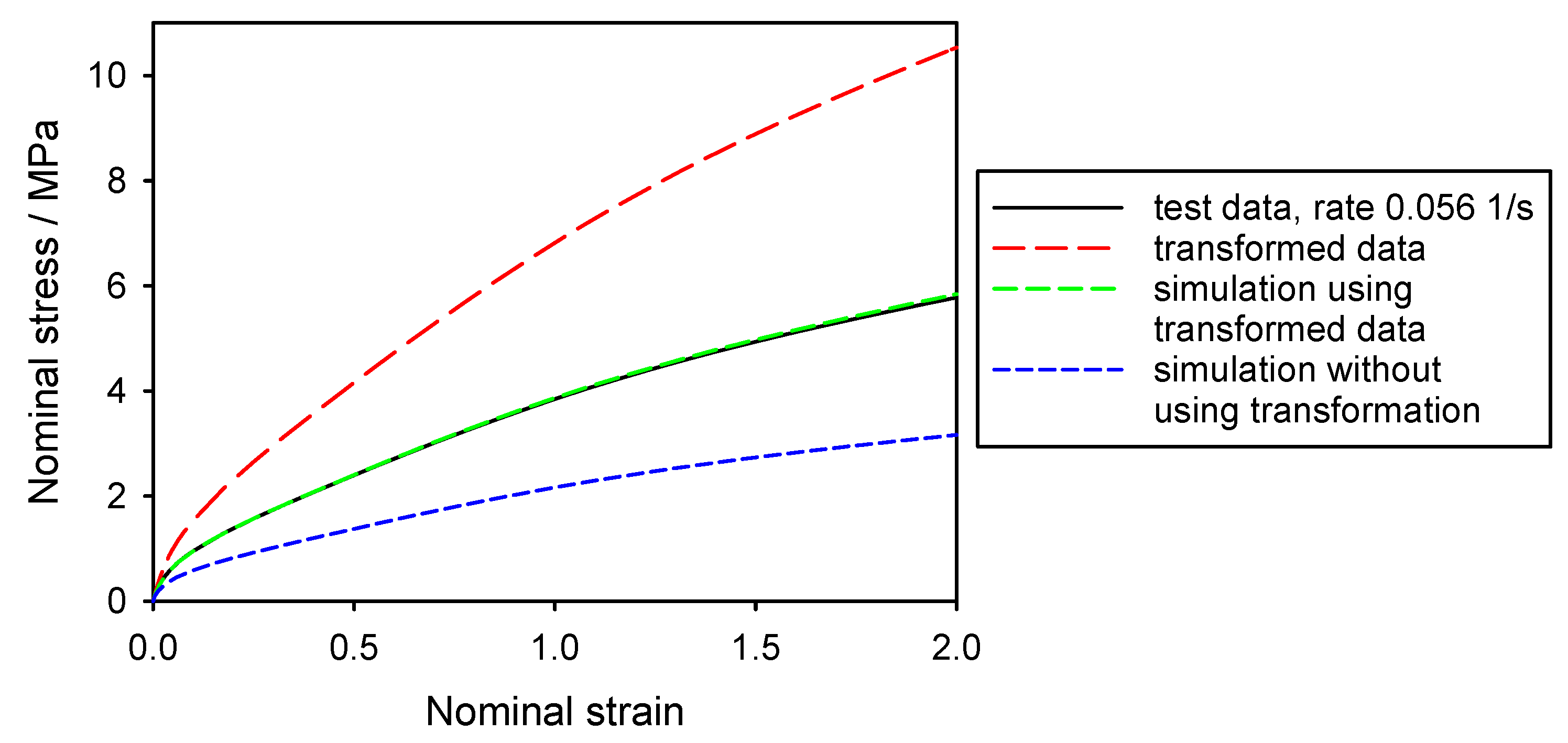
An example of an application of the implemented method is displayed in Figure 1. The black curve is the nominal stress–strain curve of a tensile test at a constant strain rate. The test data was measured for a polyurethane adhesive [19], but in the context of this paper, it shall be considered just as a numerical test of the developed method. Additional to this stress–strain curve, parameters defining the viscoelastic properties and the compressibility were obtained from a relaxation test and a hydrostatic compression test. The parameters of the Prony series and the bulk modulus are shown in

Table 1. Prony series parameters and bulk modulus of the example.

${\mathit{g}}_1$	${\mathit{\tau }}_1$	${\mathit{g}}_2$	${\mathit{\tau }}_2$	${\mathit{g}}_3$	${\mathit{\tau }}_3$	${\mathit{g}}_4$	${\mathit{\tau }}_4$	${\mathit{g}}_5$	${\mathit{\tau }}_5$	K
	in s		in s		in s		in s		in s	in GPa
0.3539	0.08124	0.07458	1.692	0.05052	35.23	0.04117	733.5	0.04575	15275	2.5

.

The result of the transformation of this exemplary data is shown by the red dashed curve in Figure 1, which is the instantaneous stress–strain curve of the viscoelastic Marlow model. The Python program implementing the proposed method generated an input file for the finite element software [18] defining the material model. In finite elements, a one element test of the model was performed using a uniaxial tensile loading at the strain rate of the original tensile test. The nominal stress–strain curve of this simulation is displayed as a green dashed line. It agrees well with the test data (black curve) with differences much smaller than the typical experimental scatter of tensile tests on elastomers.

The blue dashed curve in Figure 1 is the result of another one-element test using the visco-hyperelastic model. In this case, the transformation suggested in this paper was not used, but the tensile test data was directly supplied as input of the Marlow model, while the same viscoelastic properties were specified as before. The simulation using this model significantly differs from the test data.

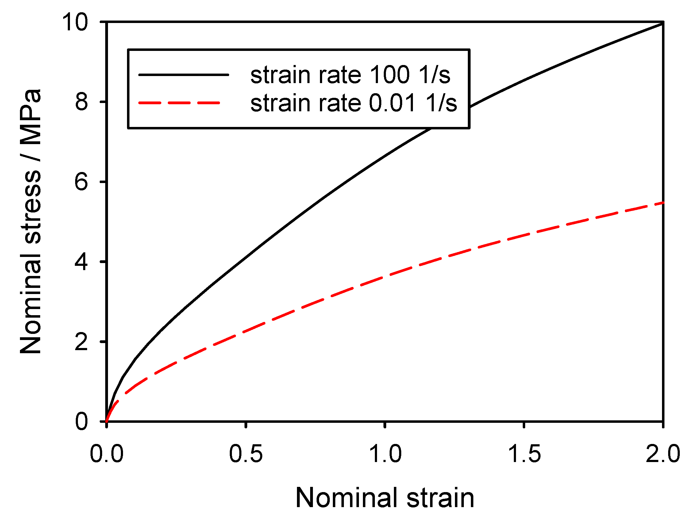
In order to illustrate the difference between the viscoelastic Marlow model and the standard Marlow model, Figure 2 shows results of the model under uniaxial tensile loading at two different strain rates. A Marlow model without viscoelasticity predicts the same stress–strain curve for all strain rates, which agrees with experiments at the strain rate used for its calibration. The amount of strain-rate dependence depends on the specific material and the temperature, of course.

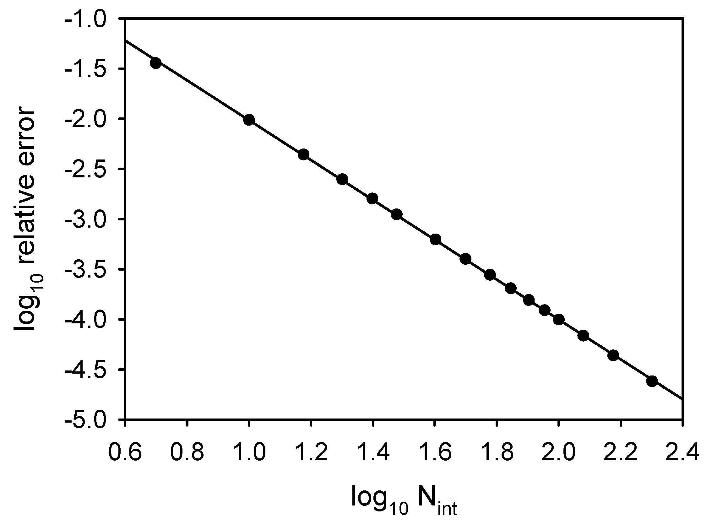
The implementation of the method contained numerical integration using the trapezoidal rule with a uniform grid. Its accuracy depends on the number of intervals, $N_{int}$. The same numerical example as before was used to study the convergence of the numerical integration. The input data for the viscoelastic Marlow model was calculated using different values of $N_{int}$. For each value, the tensile test was simulated. The difference of the simulated stress and the test data was evaluated at the upper end of the stress–strain curve. Figure 3 shows the difference relative to the absolute value of the stress, i.e., the relative error of the numerical approximation. The slope of the regression curve in the log–log-plot is −1.99, which means that the error decreases approximately quadratically with increasing $N_{int}$.

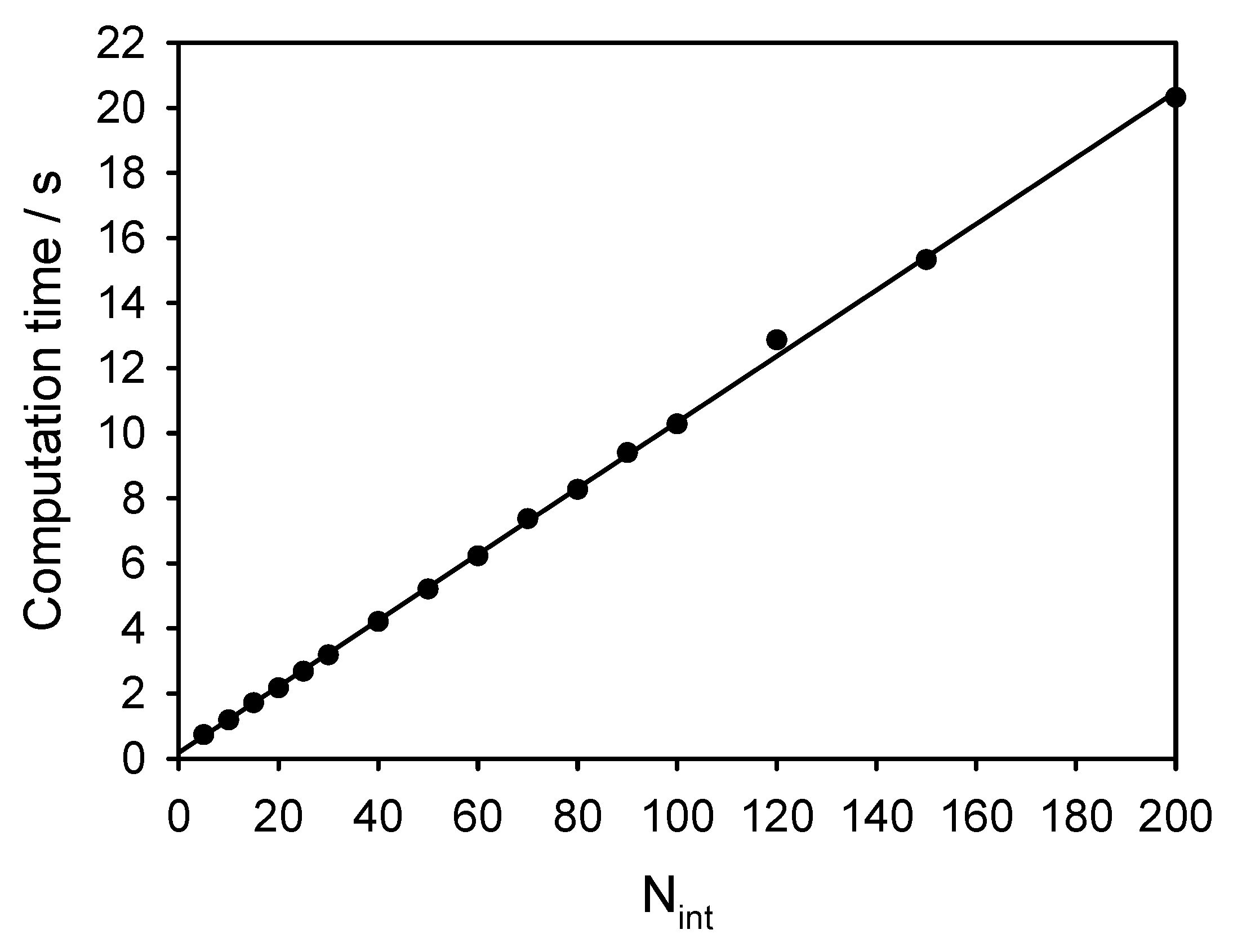
The time required to perform the computation is displayed in Figure 4. It grows linearly with the number of intervals $N_{int}$. With the choice $N_{int}=50$, the computation time on an ordinary PC was only 5 s and the relative error only $4\times {10}^{-4}$.

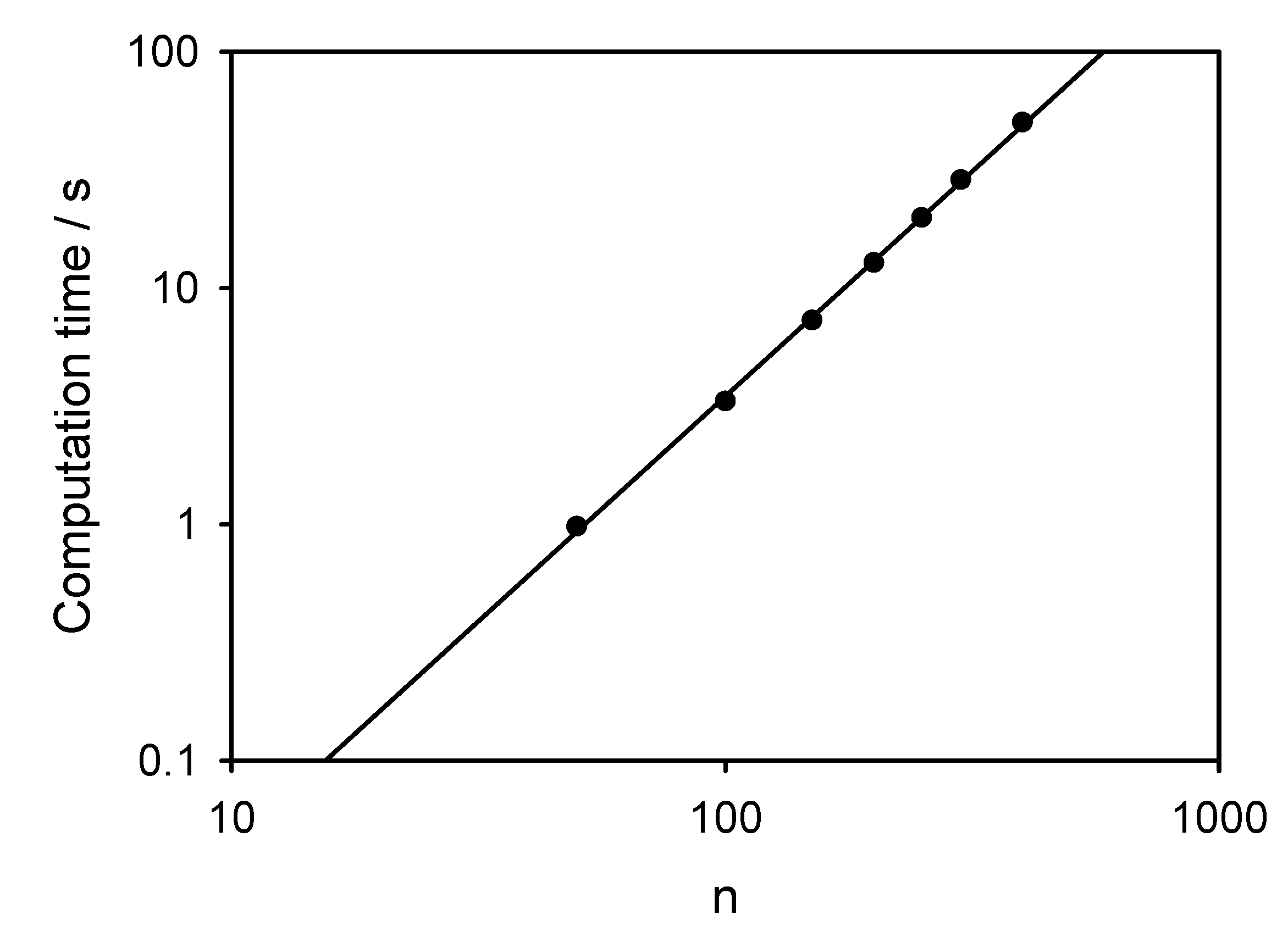
The number of required numerical integrations $n(n+1)$ grows quadratically with the number of points n of the stepwise linear approximation of the stress–strain curve. The computation time as displayed in Figure 5 shows a similar increase with a slope of 1.9 in the log–log-plot.

Therefore, n should not be chosen larger than necessary. Values n between 100 and 300 are reasonable and result in computation times below half a minute on an ordinary PC. The computation method does not require the stretch points ${\lambda }_k$ to be uniformly spaced. It is advisable to choose smaller intervals at the start of the stress–strain curve where its slope is higher than at the end.

3. Discussion

The viscoelastic Marlow model combines the advantages of the hyperelastic Marlow model and the consideration of stress relaxation:

• The model describes strain-rate dependence of the mechanical behavior.
• The model can be defined so that it fits exactly to the result of one experiment, e.g., a tensile test. In contrast, hyperelastic models based on a small set of parameters like polynomial models or Ogden’s model exhibit significant deviations from experimental data for some materials.
• The parameter identification is direct in the sense that it requires no optimization procedure. Consequently, the result does not depend on parameters of an optimization like the choice of an absolute or relative error measure, the optimization algorithm, or the initial values.

The calculation method proposed in this paper was developed with the aim to maintain the Marlow model’s advantage of direct parameter identification in the viscoelastic Marlow model. It is basically a transformation from a uniaxial stress–strain curve at constant strain rate to the curve describing the instantaneous hyperelastic response. This method was implemented as a Python program and verified. It requires the nominal stress–strain curve of a tensile test at an arbitrary, constant strain rate as input and yields the material card for the employed finite element program as an output. This computation needs only a couple of seconds, so the method is very convenient.

Additionally required parameters of the computation are the Prony series parameters describing the viscoelasticity and the bulk modulus determining the volumetric behavior. This implies the limitations of the developed method: The parameter identification remains direct only if the additional parameters can be identified independently.

The Prony series parameters can be obtained from a relaxation test, where a constant strain is applied instantly and the relaxation of the stress over time is measured. A straightforward evaluation of this test is to interpret the normalized stress over time as the normalized relaxation function and to fit it using the Prony series. This approach assumes that the decrease of the normalized stress over time is not significantly influenced by the nonlinearity of the hyperelastic part of the material model. The assumption looks reasonable if the applied strain is chosen as small as possible, but its accuracy still needs to be investigated systematically.

Concerning the volumetric behavior, a limitation of the developed procedure is that a constant bulk modulus is assumed. A model of the volumetric behavior with only a single parameter was chosen, because accurate hydrostatic pressure tests are difficult to perform, so it is difficult to identify more sophisticated models uniquely. It is possible to adjust the method to other volumetric models. For example, the employed finite element software allows for defining a Marlow model specifying a Poisson’s ratio that remains constant for all strains in uniaxial tension. A similar method was implemented for this kind of volumetric model behavior but is not shown in this paper.

The bulk modulus can be identified separately in a hydrostatic compression test. The instantaneous bulk modulus can be calculated from the value measured at constant strain rate using the Prony series. However, if the elastomer is nearly incompressible, deformation of the test setup and perhaps friction may influence the measurements in a hydrostatic compression test. Then, an accurate evaluation of the test might require a finite element simulation and an optimization of the bulk modulus as model parameter. This is no shortcoming of the calculation method proposed in this paper, but a specific difficulty of the hydrostatic compression experiment.

4. Materials and Methods

The computer algebra system Mathematica [20] assisted in deriving the transformation and double-checking the results. The transformation was implemented using the programming language Python [21]. In the numerical test of the material model generated using the method proposed in this paper (Figure 1), the finite element software Abaqus [18] was used.

References

- Marckmann, G.; Verron, E. Comparison of Hyperelastic Models for Rubber-Like Materials. Rubber Chem. Technol. 2006, 79, 835–858. [Google Scholar] [CrossRef] [Green Version]
- Martins, P.A.L.S.; Natal Jorge, R.M.; Ferreira, A.J.M. A Comparative Study of Several Material Models for Prediction of Hyperelastic Properties: Application to Silicone-Rubber and Soft Tissues. Strain 2006, 42, 135–147. [Google Scholar] [CrossRef]
- Vahapoğlu, V.; Karadeniz, S. Constitutive Equations for Isotropic Rubber-Like Materials Using Phenomenological Approach: A Bibliography (1930–2003). Rubber Chem. Technol. 2006, 79, 489–499. [Google Scholar] [CrossRef]
- Steinmann, P.; Hossain, M.; Possart, G. Hyperelastic models for rubber-like materials: Consistent tangent operators and suitability for Treloar’s data. Arch. Appl. Mech. 2012, 82, 1183–1217. [Google Scholar] [CrossRef]
- Chagnon, G.; Rebouah, M.; Favier, D. Hyperelastic Energy Densities for Soft Biological Tissues: A Review. J. Elast. 2015, 120, 129–160. [Google Scholar] [CrossRef] [Green Version]
- Marlow, R.S. A general first-invariant hyperelastic constitutive model. In Constitutive Models for Rubber III; Busfield, J., Ed.; Balkema: Lisse, The Netherlands, 2003; pp. 157–160. [Google Scholar]
- Arruda, E.M.; Boyce, M.C. A three-dimensional constitutive model for the large stretch behavior of rubber elastic materials. J. Mech. Phys. Solids 1993, 41, 389–412. [Google Scholar] [CrossRef] [Green Version]
- Yeoh, O.H.; Fleming, P.D. A new attempt to reconcile the statistical and phenomenological theories of rubber elasticity. J. Polym. Sci. Part Polym. Phys. 1997, 35, 1919–1931. [Google Scholar] [CrossRef]
- Esposito, M.; Sorrentino, L.; Krejčí, P.; Davino, D. Modelling of a visco-hyperelastic polymeric foam with a continuous to discrete relaxation spectrum approach. J. Mech. Phys. Solids 2020, 142, 104030. [Google Scholar] [CrossRef]
- Iqbal, M.; Li-Mayer, J.; Lewis, D.; Connors, S.; Charalambides, M. Mechanical characterization of the nitrocellulose-based visco-hyperelastic binder in polymer bonded explosives. Phys. Fluids 2020, 32, 023103. [Google Scholar] [CrossRef]
- Luo, Y.M.; Chevalier, L.; Monteiro, E.; Yan, S.; Menary, G. Simulation of the Injection Stretch Blow Molding Process: An Anisotropic Visco–Hyperelastic Model for Polyethylene Terephthalate Behavior. Polym. Eng. 2020, 60, 823–831. [Google Scholar] [CrossRef]
- Ramzanpour, M.; Hosseini-Farid, M.; Mclean, J.; Ziejewski, M.; Karami, G. Visco-hyperelastic characterization of human brain white matter micro-level constituents in different strain rates. Med. Biol. Eng. Comput. 2020, 58, 2107–2118. [Google Scholar] [CrossRef] [PubMed]
- Hesebeck, O.; Wulf, A. Hyperelastic constitutive modeling with exponential decay and application to a viscoelastic adhesive. Int. J. Solids Struct. 2018, 141, 60–72. [Google Scholar] [CrossRef] [Green Version]
- Ogden, R.W. Large deformation isotropic elasticity—On the correlation of theory and experiment for incompressible rubberlike solids. Proc. R. Soc. Lond. A. Math. Phys. Sci. 1972, 326, 565–584. [Google Scholar] [CrossRef]
- Zwanzig, R.; Mountain, R.D. High–Frequency Elastic Moduli of Simple Fluids. J. Chem. Phys. 1965, 43, 4464–4471. [Google Scholar] [CrossRef]
- Puosi, F.; Leporini, D. Communication: Correlation of the instantaneous and the intermediate-time elasticity with the structural relaxation in glassforming systems. J. Chem. Phys. 2012, 136, 041104. [Google Scholar] [CrossRef] [PubMed] [Green Version]
- Dyre, J.C.; Wang, W.H. The instantaneous shear modulus in the shoving model. J. Chem. Phys. 2012, 136, 224108. [Google Scholar] [CrossRef] [PubMed] [Green Version]
- Dassault Systèmes. Abaqus 2019. 2019. Available online: https://www.3ds.com/products-services/simulia/products/abaqus (accessed on 1 November 2020).
- Hesselbach, J.; Hesebeck, O.; Carrillo Beber, V. Geklebte Langzeitstabile Organoblech-Aluminium-Knotenverbindungen und deren Berechnung mit Einem Erweiterten Arruda-Boyce Werkstoffmodell; Report of IGF Project 19609 N; in preparation.
- Wolfram. Mathematica 11.1. 2017. Available online: https://www.wolfram.com/mathematica (accessed on 1 November 2020).
- Python 3.6.0. 2017. Available online: https://www.python.org (accessed on 1 November 2020).
Figure 1.
Example stress–strain curves showing tensile test data, transformed data, and verification.
Figure 2.
Example stress–strain curves depending on the strain rate.
Figure 3.
Relative model error depending on the number of numerical integration intervals.
Figure 4.
Computation time depending on the number of numerical integration intervals.
Figure 5.
Computation time depending on the number of points n of the stress–strain curve.