Towards Spatial Composite Indicators: A Case Study on Sardinian Landscape


Department of Civil and Environmental Engineering and Architecture (DICAAR), University of Cagliari, 09123 Cagliari, Italy
*
Author to whom correspondence should be addressed.
Sustainability 2018, 10(5), 1369; https://0-doi-org.brum.beds.ac.uk/10.3390/su10051369
Submission received: 27 March 2018
/
Revised: 22 April 2018
/
Accepted: 23 April 2018
/
Published: 27 April 2018
(This article belongs to the Special Issue Sustainable Land Uses and Rural Governance)
Abstract
:Composite Indicators (CIs) recently earned popularity as decision-support tool in policy-making for their ability to give concise measures of complex phenomena. Despite growing diffusion of the use of CI in policy-making, current research has barely addressed the issue of the spatial dimension of input data and of final indicator scores. Nowadays the spatial dimension of data plays a crucial role in analysis, thanks to recent developments in spatial data infrastructures which has enabled seamless access to a large amount of geographic information. In addition, recent developments in spatial statistical techniques are facilitating the understanding of the presence of spatial effects among data, spatial dependence and spatial heterogeneity. These advances are improving our ability to understand the spatial dimension of information, which is crucial to obtain a more robust representation of the territorial reality and insights of territorial dynamics in order to inform decisions in spatial planning and policy-making. This paper proposes an original method for the integration of spatial multivariate analysis and the use of spatial data to extend existing state of the art methods for CIs, as a step towards the construction of Spatial Composite Indicators. The method was successfully tested on a landscape planning case study.
1. Introduction
In general terms, a Composite Indicator (CI) represents a measure that encompasses the collective character of simultaneous and different dimensions of a certain aspect of reality. The Joint Research Center defines composite indicators as “an aggregate index comprising individual indicators and weights that commonly represent the relative importance of each indicator” [1]. Tarantola and Saltelli (after Hammond, 2008) [2] define an indicator as a measure of some characteristics of reality that are not immediately detectable. In other words, a composite indicator is the result of the mathematical combination of individual indicators that represents different dimensions of a concept, the description of which is the objective of the analysis [3]. Saltelli [4] indicates sensu lato a composite indicator as a manipulation of different indicators to produce an aggregate ordinal or cardinal measure of the performance of administrative units most commonly at the national level.
To date, CIs have mainly been used to assess the level of socio-economic performance of countries, and to support evidence-based policy making. Nowadays, the use of composite indicators is facing an increasing interest that may be attributed to different advantages [1], including:
- Capacity of CI to summarize complex and multidimensional issues;
- Capacity to provide a big picture about a certain phenomenon and to facilitate the construction of a rank for spatial units, usually countries or other administrative units, on complex issues;
- Capability to attract public interest;
- Effectiveness in reducing the size of a list of indicators.
Despite their several potential advantages, CIs are still subject to debate in the scientific community, specifically regarding existing discordances about their use. The first issue of concern regards the fact that CIs are models which represent a certain aspect of the reality; hence, CIs may represent different legitimate and contrasting perspectives by different stakeholders. This highlights the fact that, in the use of CIs, negotiation among stakeholders has to be reached in order to clearly define the structure and the intended semantic of the indicator; therefore, CIs cannot be considered only as an aggregation of numbers [1]. This point is crucial to send the correct political message by means of CIs. The second point of debate concerns the fact that, as a model, CIs are subjected to uncertainty [5]. The third point of discordance concerns the different scientific positions between aggregators and non-aggregators. Aggregators support the use of CIs because of their capability to capture and summarize the complexity of the reality; usually the CIs are driven by the need of advocacy, whose rationale can be mainly identified in the generation of narratives supporting the subject of the advocacy.
Non-aggregators conversely support the hypothesis that a set of individual indicators is sufficient to support information in policy and decision making [6]. In addition, they criticize the use of weights to combine the variables, because of the arbitrary nature of weighting procedure [4].
Notwithstanding the debate on the opportunity to use CIs in policy and decision-making, with the due precautions to address the issues outlined above, in several domains the advantages on using CIs are evident [7,8,9,10,11,12].
There is not a standard methodology to build CIs. Nevertheless, the Organization for Economic Co-operation and Development (OECD) and the Joint Research Centre of the European Commission (JRC), two institutions which have been making large use of CIs, supply guidelines for their construction. As a mathematical model, the construction of CIs follows a sequence of steps; each step can be developed in various ways, although methodological coherence should be ensured in the overall process.
According to the guidelines provided by the OECD and the JRC [13] the construction of the step involved in the construction of CIs are:
- Formalization of the theoretical framework;
- Data selection;
- Imputation of missing data;
- Multivariate analysis;
- Weighting and aggregation;
- Uncertainty and sensitivity analysis;
- Back to the original data;
- Link to other indicators;
- Visualization of the result.
Most of these steps are developed by the use of statistical techniques, as in case of the imputation of missing data, of the multivariate analysis, of the weighting, and of the uncertainty and sensitivity analysis. Usually, the construction of composite indicators involves the use of socio-economic dataset, but the spatial dimension of data is considered neither with regards to data nor for analysis. However, recent development in spatial statistics techniques makes actual the possibility to expand the methodology in order to incorporate the study of the spatial dimension into the CIs’ building process. This opportunity is made further urgent by the potential for exploiting the growing availability of interoperable spatial data made available, thanks to recent developments in Spatial Data Infrastructures (SDI), such as in the case of the European INSPIRE SDI [14] to support environmental protection policies and spatial governance and decision-making [15].
Towards Spatial Composite Indicators
The literature review reveals that little attention has been paid to the study of the spatial dimension of CIs and of the constituting variables involved in the building process. In building CIs, the input variables are commonly considered as average attribute values of geo-referenced administrative spatial unit. However, seldom environmental, economic and social phenomena unfold uniformly within given conventional boundaries. Therefore, the actual unprecedented availability of large scale spatial data representing real-world objects and phenomena offers the opportunity to make value of the spatial dimension of input variables enriching the modeling and analytical power for CIs to become spatial.
The analysis of the spatial dimension of data is becoming a crucial point for both spatial and socio-economic data [16] thanks to the rapid changes in perceived space, to the improvements in technologies, and to the change in political landscapes [17]. Currently, the development in the provision and quality of digital data create new opportunities for spatial and temporal measures at a finer level of detail than in the past, including large intra-urban scales [18]. Recent studies on Spatial Decision Support Systems [19,20] have demonstrated how spatial multi-criteria indicators can be used to represent complex phenomena in order to help stake-holders’ complex decisions in physical planning. However, in the study of the spatial dimension, the location where data were collected is very important, because it creates a link among the value of the data, their position, and their values in the nearest location. This aspect brings to two important spatial effects: spatial heterogeneity and spatial dependence [16,21]. Spatial heterogeneity and spatial dependence invalidate the basic statistics assumption of the independence of data and of the random distribution of data across space [16,22,23,24,25]. The effect of the data location makes it necessary to treat spatial data by means of particular spatial statistical methods, which are able to capture the special nature of spatial data, to discover spatial patterns, and to identify various spatial regimes and other forms of spatial non-stationary [23].
Various empirical studies proved the importance of the spatial dimension to better understand the reality. Mainly, the focus of these studies is the finding of spatial relations among various social characteristics, often social disadvantage, in order to achieve deeper spatial information on the spatial behavior of social indicators and their mutual spatial relationship [18,26,27,28].
In the specific case of CIs, spatial analysis has been barely applied. However, spatial information may enable policy makers to make more robust and more effective decisions [29]. Two case studies appear particularly interesting: (i) the application of spatial autocorrelation for the Regional Competitiveness Index (RCI) [30]; and (ii) the study of social vulnerability to malaria in East Africa [31]. In the first case, the analysis of the spatial dimension was carried out after the calculation of the overall CI. The aim was to discover clusters with similar behavior among the EU regions (i.e., the chosen administrative spatial units) and the presence of spillover regions. Additionally, the study focused on the detection of the spatial relationships between CI and its sub-dimension.
In the case study on social vulnerability to malaria, the aim was to distinguish areas on the basis of the risk of malaria. The use of the concept of geoms [32] allowed for the identifying of homogenous spatial units of analysis. Geoms are homogeneous spatial objects defined in terms of spatial variation of phenomena under the influence of policy interventions, generated by scale specific spatial regionalization of a complex and multidimensional geographical reality, and incorporating expert knowledge [26]. With this attempt, the malaria vulnerability study represents an early proposal to introduce the study of spatial dimension in the construction process of the CIs.
A common point of the studies presented above, is the fact that the assignment of the weights is not local. It means that the spatial variation of the importance of the variables that compose the final indicator is not detected; once weights are assigned, they are kept constant in each location. In the RCI case study, the weighting procedure adopted equal weights based on a previous Principal Component Analysis (PCA), while in the case of Malaria Vulnerability, the weights were set by experts. The case studies offer two examples of the two alternative weighting procedures: the data-driven methods, as in the case of RCI, and the knowledge-driven methods, as in the case of the Malaria study [33].
To the first group belong to those methods based on data mining techniques, which seek to identify trends in the hierarchy of variables according to what happens in reality, measured by samples chosen to investigate the territory [34]. Conversely, in the knowledge driven approach, the goal is to receive feedback by experts on the investigated phenomenon [35].
In light of the above premise, it appears urgent to investigate the possibility to improve the methodology for the construction of CIs. Such a methodology should be able to take into account both the spatial effects due to the use of spatial data, and their consequences in the assignment of weights, in order to have a set of local weights based on the spatial variability of data. To achieve this goal, an extension of the OECD/JRC methodology is proposed and tested on the case study of the landscape in Sardinia.
2. Methods
2.1. The Integration of Spatial Statistics to Account for the Spatial Dimension in SCIs
The special nature of spatial data and its effects (spatial dependence and spatial heterogeneity) invalidate the hypothesis of random distribution of variables across the space, creating a spatial non-stationary condition. This condition may affect also the local importance of variables, invalidating the use of constant weights. In addition to this, spatial relations among the spatial units have to be studied in a spatial way in order to understand where the effect of spatial non-stationary creates a spatial cluster. Indeed, there is a need to treat spatial data with specific techniques which are able to consider the mentioned spatial effects. Recent development in spatial statistics offers new methods that may contribute to the achievement of this goal. Replacing some steps in the original OECD/JRC methodology with these novel spatial statistical methods, it is expected to improve the capability of CIs to provide a richer “spatial” picture of certain phenomena by means of more detailed spatial information. Table 1 shows the comparison between the OECD/JRC, and the spatially-enabled version of the methodology. The main conceptual difference between the two is the introduction of spatial data as input datasets and the application of the Geographically-Weighted Principal Component Analysis (GWPCA) in replacement of the traditional multivariate analysis. GWPCA is a quite recent technique that represents the local form of PCA [36]. It assumes that there may be various regions in which it is needed to apply different and distinct PCA in order to take into account local variation (non-stationary spatial condition) on the set of data. This way it is also possible to explore the internal structure of spatial data. Indeed, GWPCA provides a locally-derived set of principal components at all data locations [37]. In addition, GWPCA returns, for each component the so called variable loading, which has been used to obtain local weights, as will be shown later in the case study section.
In order to be applied, the GWPCA needs a preliminary calibration in order to minimize the distance between the original data and the obtained components. The calibration is carried out by the research of the so-called bandwidth, which can be defined as a fixed quantity (in terms of spatial units) that reflects local sample size [38].
A further difference between the two methodologies is that in the spatial case, some steps are carried out in different sequence order than in the traditional non-spatial case.
The different order in the implementation of some steps is specifically required by the use of spatial data. A relevant example is data normalization: in the spatial case it is recommended to perform the normalization before carrying on the spatial multivariate analysis, because the effect of the use of non-normalized data in GWPCA is still subjected to further research [38].
Finally, spatial autocorrelation is used to detect spatial clusters with similar behavior of the indicator’s value [30]. Local spatial autocorrelation, both univariate and bivariate, is then used to take into account also the spatial relation between the value of the indicator and the data used for the CI construction, and in order to identify locations in which spatial autocorrelation is significant [39].
2.2. Case Study: Landscape
The methodology proposed has been tested on the case of the landscape in Sardinia. Landscape has been chosen as the case study because it can be considered both a spatial and a complex phenomenon. In addition, landscape preservation is currently a priority informing the development of spatial development policies in the region.
According to the methodology proposed by OECD/JRC, the first important step in the construction of a composite indicator (be it spatial or not) is to build a robust theoretical framework for the indicator. The construction of the theoretical framework starts from a clear definition of the phenomena that the indicator is intended to describe, in order to identify the various dimensions that compose it.
Defining landscape is not an easy task, because it is the result of an ongoing interaction of several aspects, involving natural, anthropogenic and perceptive dimensions [40,41]. Landscape is a holistic, dynamic and abstract concept. It has no defined borders despite the fact that it is possible to recognize various types of landscape in a topological sense [40]. The intrinsic complexity of the landscape is proven by the large number of approaches used in landscape studies. Most of the approaches focus only on one or a few (if compared with the large number of aspects involved) particular aspects of the landscape: different approaches which consider landscape from either an ecological, or a cultural or a perceptive perspective are found. However, the various approaches are barely integrated together, despite the fact that the integration among them appears to be essentially relevant in order to try to consider all the landscape dimensions at the same time [42].The need to have a holistic representation of the landscape, which may be able to consider simultaneously the physical, cultural and perceptive aspects, is suggested also by the European Landscape Convention, which states: “Landscape means an area, as perceived by people, whose character is the result of the actions and interaction of natural and/or human factors [43].
The European Landscape Convention puts more emphasis on the fact that landscape is a resource in which local communities have formed their own culture, creating and modifying the various places that compose the overall European landscape. Hence, great attention should be paid to landscape protection. However, landscape is a dynamic process that changes continuously and inevitably due to both natural and human factors. Often, human modifications are responsible for the fastest landscape changes. Mankind modifies landscape to satisfy the need for food, housing and services. In some cases, these changes may be undesirable in terms of their consequences on environmental or on cultural features.
According to Steiner (2000) [44], indicators are the best tools to understand and to measure the alterations of landscapes and their consequences. Unfortunately, the complexity of landscape does not make its description easy by means of indicators. The main difficulty is to understand exactly which indicators should be measured. In general terms, the objective is to obtain indices able to provide information about the state of the environment and about the consequences in landscape structure and landscape functions [41]. Another difficulty in landscape measures comes from the dynamic nature of landscape: for the calculation of indicators it is necessary to specify both the spatial and the temporal scale [45,46]. The spatial scale refers both to the extension of the study area and to the choice of the basic spatial units of analysis. The spatial scale strongly influences the relevance of the landscape factors and also their behavior across space [46,47,48]. The temporal scale determines how landscape patterns change overtime, in order to discover the causes of the landscape evolution and also its causes and consequences on the landscape [49]. In addition, it is difficult to assess the significance of a pattern measured at one point, without considering the historical variability of the pattern [45].
Landscape indicators can be divided in two main groups [41,50]: the indicators about the physical and the ecological characteristics and the indicators about the visual, the social and the cultural aspects. The first group focuses on the objective components of the landscape such as the landscape structure, and the physical/ecological landscape functions. The landscape functions aim to describe how landscape changes affect the species and the communities; furthermore, a prerequisite to understanding landscape functions is the comprehension of the landscape structure [51,52].
The landscape structure concerns two important aspects: composition and configuration [50]. Composition refers to the non-spatially-explicit characteristics of landscape (richness, evenness, diversity), while configuration is related to the spatially-explicit characteristics of the land cover type in a given area; the latter are associated with patch geometry or with the spatial distribution of patches. Landscape metrics are the most used indicators for the physical/ecological characteristics of a landscape. Landscape metrics are a selection of indicators mainly developed in Landscape Ecology [52,53] with the aim of evaluating the state of the landscape from an ecological point of view, that is, to understand the effect of changes on the landscape structure and on the landscape functions.
Landscape metrics should be not interpreted individually, but in combination with each other, in order to achieve more complete information. The optimal sub-set of landscape metrics should be chosen in order to provide the largest information set possible, but at the same time, the redundancy among metrics must be avoided. Therefore, it is necessary to choose carefully the set of indicators to use, in order to ensure the independence among them.
The second main group of landscape indicators focuses mainly on the perceived aspects of landscape. Quantifying the perceived aspects of the landscape is not an easy task. The main difficulty relies on the fact that perception is inevitably subjective, because people see and appreciate the landscape in different ways. Therefore, the appreciation of the landscape might vary on the basis on the involved observers. Indeed, the most commonly used way to collect data about landscape appreciation is through questionnaire-surveys. This is one of the main limits responsible for the shortage of indicators measuring landscape perception [54,55]. The perceived landscape encompasses also the so-called cultural landscape, which can be defined as a portion of land in which human activities created a particular system of patterns [56]. The main threats for cultural landscape are the changes caused by socio-economic factors, such as modifications in agricultural and forestry practice or human disturbances such as urban sprawl. These changes might bring to the loss of cultural landscape [57].
The European Landscape Convention brings the social and cultural dimensions of landscape to the forefront for the landscape definition, and highlights the need to develop indicators able to carefully take into account both the physical factors and the human perceptions [42]. Moreover, according to Rossler (2006) [58] cultural places cannot be considered isolated but they are part of a broadest system with the ecological aspects, creating links in space and time. Thus, on the basis of these considerations, and on the basis of the need to combine together the various indicators of landscape, the creation of a spatial composite indicator of landscape appears to be an urgent challenge.
The methodology presented in the previous section has been applied in the Oristano Province in Sardinia, Italy. The Sardinian Regional Government adopted in 2006 the first Regional Landscape Plan (RLP). In Sardinia, the planning system follows a top-down hierarchical approach, according to which any physical or sector plan should comply with the RLP in order to ensure landscape protection measures are implemented locally.
During the RLP plan-making process the Regional Government collected a large amount of spatial data setting up a regional Spatial Data Infrastructure, in compliancy with the principles and technology standards of the INSPIRE Directive (2007/2/EC). Therefore, the opportunity to build a complex landscape SCI became feasible; at the same time, it would represent a mean to demonstrate the value of having a regional SDI.
2.3. Building a Spatial Composite Indicator of Landscape
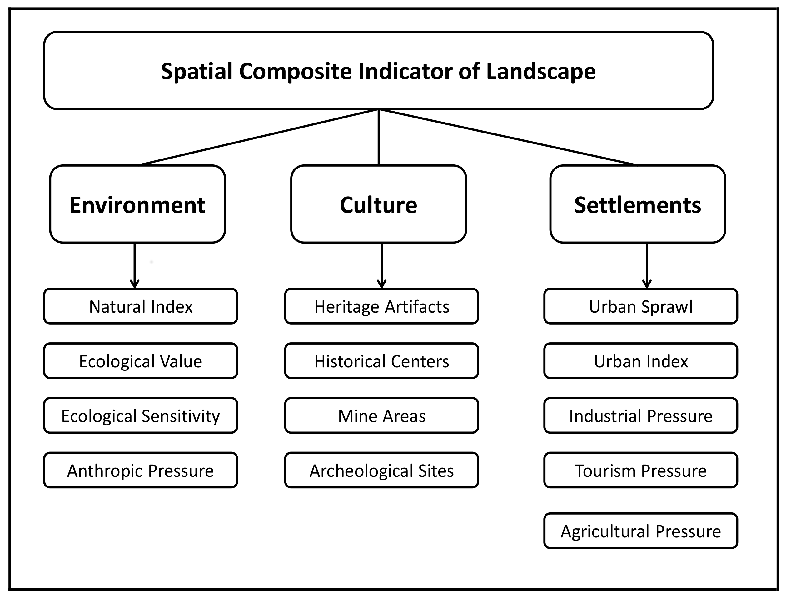
On the basis of the literature review the structure of the Spatial Composite Indicator of Landscape (SCIL) was designed relying on three main macro-dimensions: environment, culture and settlements. In turns, each macro-dimension was described by means of a selection of sub-indicators. The set of indicators to be included in each macro-dimension was driven by their relevance in the description of each macro-dimension and by the data availability (Figure 1). The main data source for the calculation of the indicators was the regional SDI of Sardinia, with the exception of the environmental macro-dimension (Table 2).
In fact, the ecological indicators (e.g., landscape metrics) strongly depends on the ecosystems or species under investigation [51], hence describing in a detailed way the ecological macro-dimension of landscape detailed data about how different species perceive the landscape are needed. Indeed, this description requires a large amount of different data in order to identify the various ecosystems for each species [51]. Despite the large amount of spatial data layers provided, the regional SDI does not supply all the data necessary for this kind of detailed analysis. To overcome this issue and to describe the environmental macro-dimension in a proper manner we used three indicators from a study called “Carta della Natura” (i.e., Nature Map) carried on by the Italian Superior Institute for the Environmental Protection and Research (ISPRA) [59]. The Nature Map identifies the main biotopes in Sardinia assessing three environmental indicators: ecological value, ecological sensitivity and anthropic pressure (Table 3).
The cultural macro-dimension quantifies those aspects of the landscape that are relevant from a historical point of view, or that created a strong link between local communities and the territory. Data used to quantify the cultural macro-dimension allow for knowing the location and size of cultural heritage or archeological sites; in seldom cases data reports and also information about the state of conservation and/or the importance of the artifacts, although this information is available only for a sub-set of records. In addition, it is not possible to achieve their level of appreciation by spatial data. Therefore, we quantify the cultural aspects on the basis of their quantity and size.
The settlement macro-dimension encompasses those aspects that, according to the literature review, create landscape disturbances. Landscape disturbances are considered all the human action able to create landscape loss in terms of landscape identity and biodiversity. The literature review mainly identified as causes of landscape disturbance the uncontrolled urban growth and the anthropic pressure in term of industrial, tourism and intensive agricultural activities.
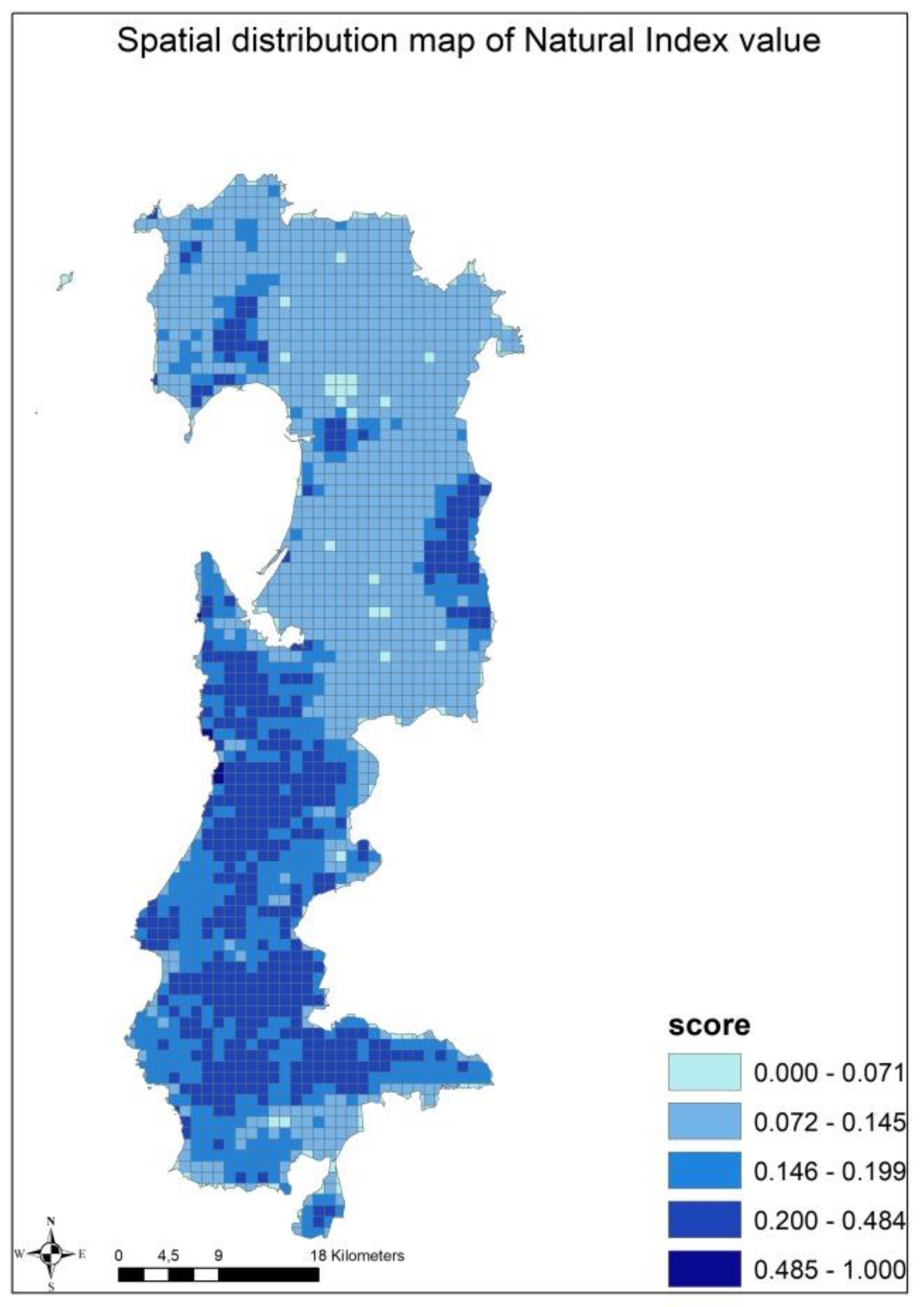
The study area which is located in the west coast of Sardinia was divided by means of a regular 1 km-size vector grid, or fishnet. Using a geoprocessing workflow, the value of each sub-indicator was calculated in each cell of the grid. In total the spatial domain is composed by 2043 cells (Figure 2). Considering that landscape “has no borders”, the use of the grid model enabled the study of the landscape without the use artificial spatial constraints, as in the case of the use administrative units, which are commonly used in CI studies.
Despite the fact that the selection of indicators may have limits in describing the overall landscape complexity, it offered the possibility to test the spatial methodology for CIs, in order to demonstrate the possibility to study the spatial dimension of the involved variables.
3. Results
Once data were collected and indicators were calculated, the creation of a composite indicator required the assessment of weights to assign to each indicator. The weights express a measure of the relative importance of the involved variable in each macro-dimension. In this particular case study, weights were assessed with a data-driven approach and locally, by the GWPCA in order to take into account the spatial effects. In addition, the use of GWPCA returns a group of variables (components) that are each other independent, enabling to avoid problems of double counting in the aggregation stage [60]. The variable loading, returned by the GWPCA for each component, reflects the local importance of the variables; hence it can be used to calculate spatial weights. At the same time the use of GWPCA allows finding out the local variance as explained by each individual component. Finally, the significance test is performed to confirm the presence of spatial heterogeneity. It is based on the assessment of the variance which comes from the randomization of the local eigenvalues; if the significance analysis returns p-values less than 0.05 it is possible to reject the null hypothesis about the random distribution of the eigenvalues. In this case it is possible to conclude that the spatial effects are relevant and the use of the GWPCA is validated [38]. Before the application of GWPCA, indicators have been standardized by using the Min-Max method, in order to make them comparable.
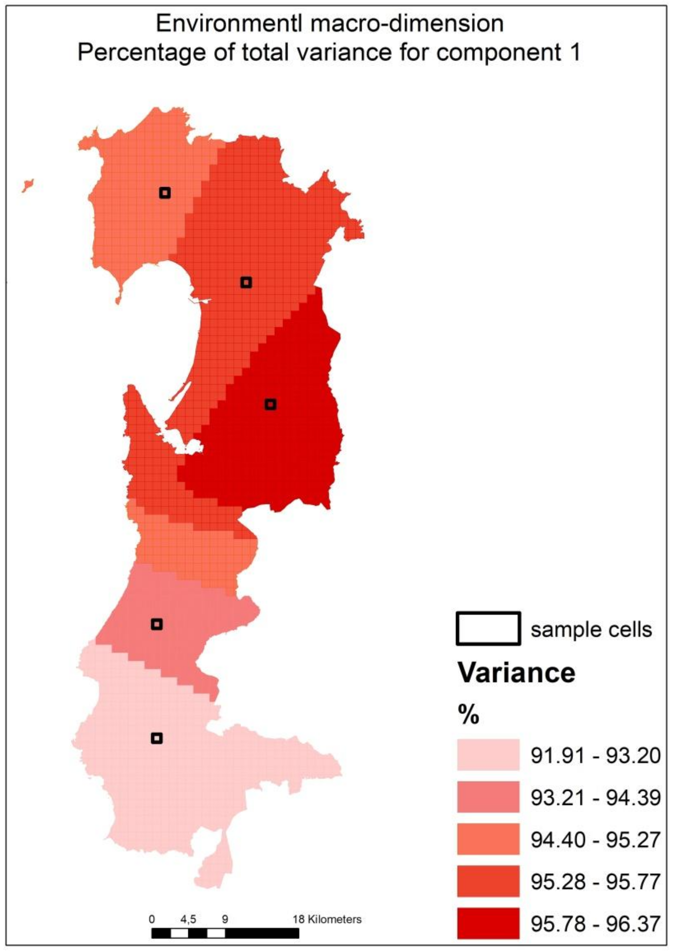
Both GWPCA and PCA were applied to each macro-dimension, in order to highlight the differences between the two methods and to put in evidence how the spatial effects influence the results of the analysis. Table 4a,b reports the comparison between the results of the GWPCA and of the PCA for the environmental macro-dimension. As it is possible to see in the example in Table 4b, with reference to the sample cells in Figure 3, in the case of the GWPCA the percentage of the total variance is returned for each spatial unit, thanks to the spatial (local) nature of this method.
According to Gollini et al. [38], the bandwidth resulting from the previous model calibration supplies the first information set about the presence of spatial heterogeneity. If the bandwidth is very small with respect to the total amount of spatial units, then it is possible to say that the effect of spatial heterogeneity is very relevant for the set of variables. Table 5 shows the resulting bandwidth for each of the three macro-dimensions. The significance analysis confirms the presence of spatial heterogeneity and the p-value it returned is less than 0.05 for each macro-dimension (Table 5). Hence it is possible to reject the null hypothesis about the spatial random distribution of the eigenvalues [38].
For all the three macro-dimensions the first extracted component explains the highest share of variation of data (Table 6), hence the variable loading of the indicator in this component has been used to assess the weights.
The value of the variable loading has been considered in absolute value and it has been rescaled so that its sum is equal to 1 in each spatial unit (Table 7). The use of the GWPCA, allowed obtaining a different set of weights for each spatial unit, which is in total 2043 sets of weights for each macro-dimension. Conversely, with the application of PCA it is possible to obtain only one set of weight across the overall spatial domain: weights are not different among spatial units, hence only a global importance of the various variables can be considered, thereby introducing uncertainty. In this sense, the use of the GWPCA can be seen as a local data-driven assessment for weights.
Once weights were obtained, the overall value of the macro-dimensions was obtained as the weighted sum (linear combination) of the variables, location by location (Equation (1)).
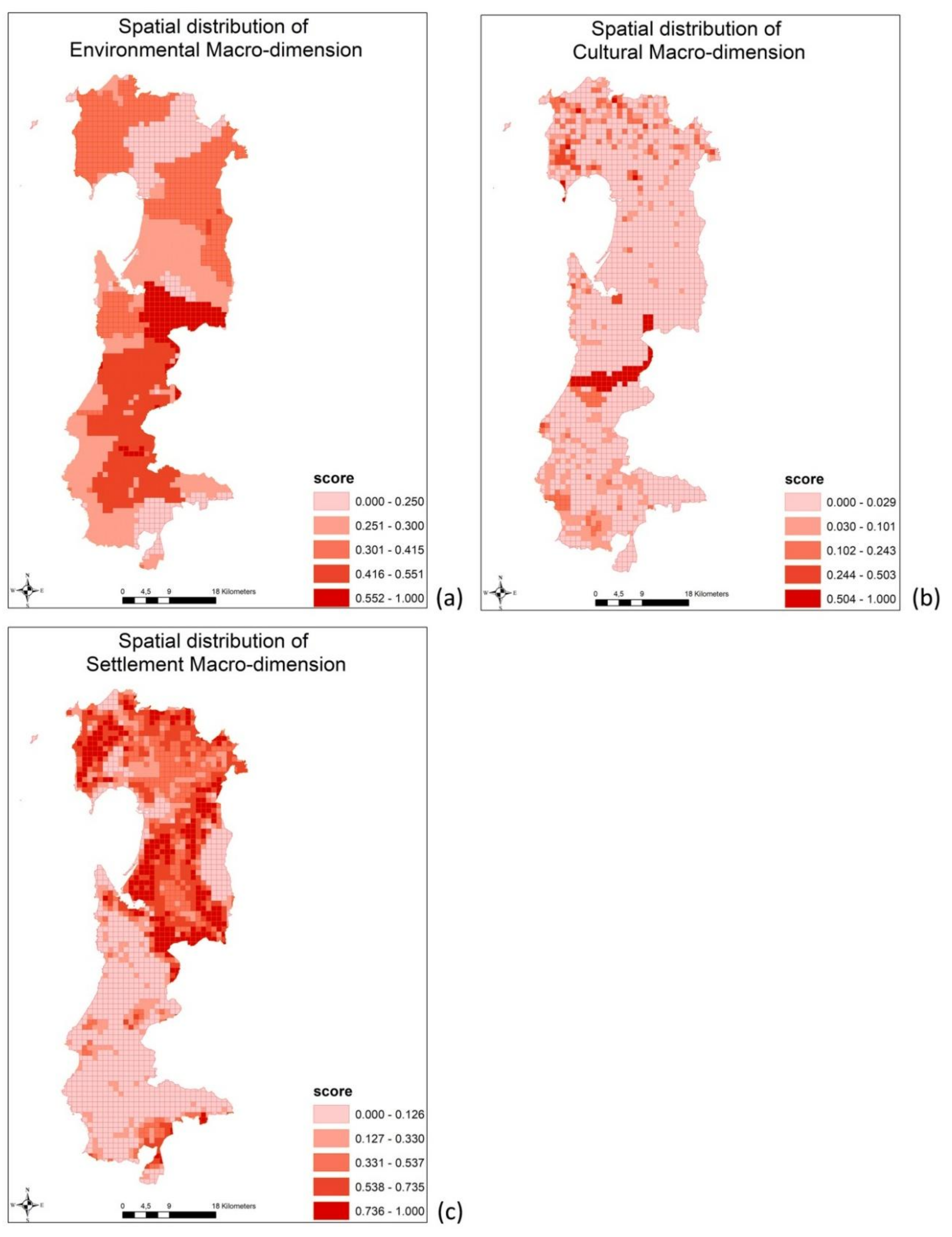
where MCj is the resulting value of the macro-dimension, ωij is the weights associate to i indicator in the j-spatial units, and I is the indicator in the j-spatial unit (Figure 4a–c). The final score of the macro-dimension has been rescaled from 0 to 1, in order to make them comparable.
The overall landscape value was assessed as linear combination of the three macro-dimensions: environment, cultural heritage and settlements.
In the Equation (2), the settlements macro-dimension have been considered as negative terms, according to the fact that in the indicator’s framework it contains the landscape disturbance [57]. The macro-dimensions have not been weighted in this case because they are considered equally important on the basis of the landscape literature review. The final result has been rescaled from 0 to 1; Figure 5 shows the spatial distribution of the final indicators of landscape, where higher values correspond to high landscape quality.
The following spatial autocorrelation analysis has been performed for the overall landscape indicator, in a univariate way, and for the indicators and their macro-dimensions, in a bivariate way, to highlight the presence of spatial dependence between the spatial units and to gain additional information about the spatial structure of the indicators. The application of local spatial autocorrelation analysis allowed detecting spatial cluster in which the presence of spatial dependence among spatial units is very significant. The evaluation of the spatial autocorrelation has been calculated using rook contiguity [61] at level 1 because it provided the highest value of the coefficient of the Moran‘s Indicator of spatial autocorrelation “I”. The results (Table 8) confirm the presence of high spatial autocorrelation in the univariate case; in the bivariate case autocorrelation was found between the SCIL and the settlement macro-dimension. In the latter case, the spatial autocorrelation is strong and negative. Conversely, in the cases of bivariate analysis between the SCIL and the environmental and cultural macro-dimensions, spatial autocorrelation is smaller than in the previous cases. Spatial clusters resulting for the local spatial autocorrelation analysis enabled to identify different types of landscape areas.
In the case of univariate analysis, it is possible to distinguish mainly two cluster types: the cluster in red represents the spatial units with high score of SCIL surrounded by spatial units with similar values of SCIL, while the blue cluster are spatial units in which the score of SCIL is low, surrounded by spatial units with low values of SCIL.
4. Discussion
The aim of the proposed methodology was to make spatial the OCED/JRC methodology for the construction of CI, in order to introduce the analysis of the spatial dimension in the description of complex territorial phenomena. The results confirm the new opportunities offered by the applications of this methodology applied in the case of landscape in Sardinia. In general, the value of this approach consists on the possibility to assign a spatial weight to each variable and to mark homogeneous areas based on the mutual spatial relation among spatial units. The methodology allowed for describing the landscape phenomenon in a spatial way. In particular, the use of spatial data from the SDI and the application of the recent spatial statistical techniques enabled to consider spatial variation of the importance of data and to understand the spatial relations among the different variables and dimensions used for the landscape description.
Landscape is a spatial phenomenon created by the continuous interactions of different aspects, which may be different depending on the spatial position and on the mutual spatial position of the variables. These variations have been confirmed by the results, which indicated a strong spatial heterogeneity on the data distribution, because of the small p-value and the small bandwidth (Table 5). The environmental macro-dimension exhibits a large bandwidth, if compared with the others two macro-dimensions. Actually, the indicators used in the description of the environmental aspect of landscape are arranged across the space in a more homogeneous manner, because they have a value in each cell of the spatial domain. Conversely the indicators of the cultural and settlement macro-dimension are allocated in a non-continuous way, because they represent punctual characteristics of the landscape or landscape aspects which themselves merge in small areas. As a matter of fact, some cells contain all indicators of the cultural or settlement macro-dimension, while in other cells only part of the set of indicators are present. The differences in the distribution of indicators in the cells produce different spatial relations among indicators depending on their local distribution; therefore, different spatial regimes are generated with the consequently spatial variation on the local importance of indicators, as it has been proven by the results (Table 6 and Table 7).
The spatial distribution of the value of the macro-dimensions substantially confirms what it was explained above. Although spatial variation is present, the environmental macro-dimension score has a more homogeneous spatial distribution (quite homogeneous mosaic) if compared with the settlement and cultural macro-dimension (Figure 5). Areas with high environmental value, in dark red, appear to be large (Figure 4a) hence it is possible to conclude that the overall study area is characterized by a high environmental quality. In case of cultural and settlement macro-dimension the mosaic of the score distribution is more heterogeneous. The spatial distribution of cultural macro-dimension score allows for identifying a high cultural level area (in dark red Figure 4b), corresponding in reality to the main mining area. In the upper part of the map, it is shown a concentration of cells with significant cultural score; these cells correspond to location where it is relevant the presence of archaeological sites, heritage buildings, and the ancient part of the towns.
The distribution of the settlement macro-dimension score clearly indicates where the anthropic disturbances on the landscape are located (in dark red in Figure 4c). These areas represent the locations in which there is a large concentration of settlements and intensive agricultural practice. Although present, the touristic and industrial disturbances are less relevant because they occupy small areas. The rest of the map indicates scarce human activities. The final indicators score summarizes the simultaneous effect of the three macro dimensions in each cell. The map of the spatial distribution of landscape quality shows that the southern part of the study area is the most remarkable, on the basis of the final score of the SCIL. Indeed, this area is characterized by scarce human presence and rich uncontaminated forest land.
The spatial autocorrelation analysis allows highlighting the spatial relation, in terms of spatial dependence among the cells, on the basis of the score of the final indicator and on the macro-dimensions and the final indicator. The purpose of the application of this technique was to identify the homogeneous areas of landscape based on the score of the indicator, in order to compare these areas with the homogenous ones identified by the RLP (Figure 6). In this sense the methodology offers a quantitative method which gave the possibility to supply further information in the process of landscape knowledge, and it may be considered complementary to the qualitative information provided by the RLP.
The main result of the spatial autocorrelation analysis is the identification of the two main kind of homogeneous areas, as shown in Figure 7a. As it is possible to see from the figure, the identified homogeneous areas by the spatial autocorrelation analysis provide a further partition of the RLP’s homogenous areas. The meaning of the spatial autocorrelation in these clusters is that there may be a contagious effect among cells. In other words, cells with high or low landscape level tend to be close together.
This tendency is exhibited also in case of bivariate analysis with the environmental macro-dimension. Substantially, cells with high environmental level are close to cells with high landscape level and vice versa (Figure 7b). In the case of the cultural macro-dimension, there are some relevant considerations that are worth to explain. Bivariate spatial autocorrelation analysis reveals the presence of a large cluster (in blue in Figure 7c), in which cultural macro-dimension indicator and the SCIL have both a low score. This behavior may be due to the fact that in this area of the study region is low on cultural aspects (Figure 4b), and at the same time, it is rich in landscape disturbances. In the upper part of the Figure 7c, the bivariate analysis highlights a situation of competition between cells. In fact, the results return cluster types with high cultural level (in pink), surrounded by cell with low landscape level; this is most likely due to the existing high human activities in these areas (Figure 4c and Figure 5). From a landscape protection point of view, this analysis suggests to pay particular attention on these areas. Indeed, the high presence of landscape disturbance may cause cultural landscape loss, if not regulated with specific planning actions. Finally, the result of bivariate analysis between the settlement macro-dimension and the SCIL, substantially confirms the theoretical framework for the Spatial Composite Indicators, in which settlement macro-dimension encompass the landscape disturbances. According to this fact, the clusters resulting from the spatial autocorrelation analysis highlight the competition between the human activities and the landscape quality, and allows identifying were this competition is relevant. Despite the fact that, in general terms, cluster types were expected, is interesting to note that there are few small red clusters. They represent portions of land in which, despite the high presence of human disturbance (settlement macro-dimension) the landscape value is high. In fact, as it is possible to note from the Figure 4a–c, these locations exhibit high scores in all the three macro-dimensions. Therefore, as suggested in the previous case of the cultural macro-dimension, particular attention has to be paid on these areas in order to propose correct policy action to preserve the landscape quality.
The combination of spatial data from Sardinian SDI with the spatial statistical techniques offered a new approach in landscape studies. The novelty of this method is the use of spatial data in a different manner than in the past, where different factors individually described spatial characteristics of the landscape without considering the mutual spatial relations among them. In this sense, the construction of a spatial composite indicator of landscape may be considered as a quantitative method that is complementary to the existing qualitative landscape assessment done by the RLP. This represents the main advantage in the construction of the spatial composite.
Despite the fact that the introduction of the spatial dimension represents an advantage for an integrated spatial description of the landscape, some controversial point still remains. The first one concerns the data issue. In general terms, composite indicators, spatial or not, are data hungry and the SDIs offer a novel and complementary data source which can be very valuable. In addition, they offer the possibility to expand the range of complex aspects of the reality to be described by means of CI. Nevertheless, in the specific case study of the landscape in Sardinia, data provided by regional’s SDI are still insufficient. The complexity of landscape, in particular the complexity of its environmental macro-dimension, requires specific data able to take into account the different landscape perception with regard to the different species. These kinds of data require sampling depending on the focus species; these datasets are not available yet in the SDI of Sardinia, which is rich of topographic data but still poor of environmental data. Another issue of concern with regards to Sardinian SDI data is that in some cases the thematic attributes are incomplete; hence it was not possible to discern many thematic characteristics. For instance, the data set of the heritage building is incomplete regarding the age of buildings or their conservation, despite the fact that the attribute table has these specific fields. For those reasons the selection of the used indicators may be considered not optimal for a deeper landscape description; still it allowed considering the main landscape aspects.
The limitation in the set of indicators leads to another criticism of the methodology, in this particular case study: the possibility to perform a good sensitivity analysis. Generally, sensitivity analysis is performed by replacing some variables or by considering one variable at time, in order to explore the behavior of the overall indicator [1]. In some cases, sensitivity analysis is carried out by discarding one of the indicators at time, while keeping all the others [31]. In other cases, sensibility is performed by application methods on spatial models in which the model is decomposed in sub groups of variables to analyze the variability of data, usually the variance of the input [62]. The scarcity of variables makes this kind of analysis (the one in which one indicator is discarded) unfeasible, while in the second kind of methods a spatial model is needed. Therefore, the question about how perform sensitivity analysis in a case where the weights are local still remains opened. In part, this lack is partially overcome by the significance analysis encompassed in the GWPCA methods. The method here presented uses only the first component extracted because it explains the most part of the variance of data, despite the fact this is not true for all the spatial units; therefore, the method needs to be improved so as to discriminate the spatial units on the basis of the winning component.
5. Conclusions
The study demonstrated that the integration of spatial multivariate analysis and the use of spatial data in the original OECD/JRC methodology for CIs can be considered an innovative step towards the construction of Spatial Composite Indicators which takes into account spatial heterogeneity and spatial dependence.
Summarizing, the presented study proposes a spatial extension of the OECD/JRC methodology for the construction of composite indicators, in order to consider the spatial consequences deriving from the use of spatial data. Recent advances in spatial statistics and broader availability of spatial data made possible to implement this new approach for Spatial Composite Indicators, which encompasses the study of the spatial dimension since the first step of the indicator’s building process. The main advantage in this sense are the capacity of composite indicators to summarize the simultaneous effect of different aspect of the realty, and at the same time the possibility to take into account the spatial effects that may occur among the variables involved in the description of these aspects. The spatially modified methodology for CIs was tested on the case study of landscape in Sardinia. Landscape has been chosen because the literature review revealed that it is a complex and spatial phenomenon, and it is a very important concept in spatial planning and policy-making. The Sardinian landscape was chosen as case study because of the growing attention of the Regional Government towards landscape protection, and of the availability of data from Regional SDI. The results confirm a strong presence of spatial heterogeneity for all the dimensions used in the definition of the SCI of landscape, in particular the cultural and the settlement macro-dimensions. The application of the local spatial autocorrelation, both in univariate and in bivariate way, on landscape SCI and its components revealed which are the groups of spatial units having either high or low landscape quality, in order to provide a new definition of valuable landscape areas. This is a crucial issue in the current season of spatial planning and policy making, in particular to support decision processes aiming at protecting areas with high landscape quality and to make decisions on how to improve the landscape quality in the other areas, by mean the identification of the factors that generate the most disturbances.
Author Contributions
This work is an outcome of joint efforts of the authors. Conceptualization: Daniele Trogu and Michele Campagna; Methodology: Daniele Trogu and Michele Campagna; Validation: Daniele Trogu and Michele Campagna; Formal Analysis: Daniele Trogu; Data Curation: Daniele Trogu; Writing-Original Draft Preparation: Daniele Trogu and Michele Campagna; Writing-Review& Editing: Michele Campagna and Daniele Trogu; Visualization: Daniele Trogu; Supervision: Michele Campagna; Funding Acquisition: Michele Campagna.
Acknowledgments
This study was supported by the research grant for the project “Healthy Cities and Smart Territories” (2016/17) funded by Fondazione di Sardegna and the Autonomous Region of Sardinia.
Conflicts of Interest
The authors declare no conflict of interest.
References
- Nardo, M.; Saisana, M.; Saltelli, A.; Tarantola, S. Tool for Composite Indicators Building; EUR 21682 EN; European Communities, Joint Research Centre Institute for the Protection and Security of the Citizen, Econometrics an Statistical Support to Antifraud Unit I-21020: Ispra, Italy, 2005; pp. 2–129. Available online: http://publications.jrc.ec.europa.eu/repository/bitstream/JRC31473/EUR%2021682%20EN.pdf (accessed on 15 March 2018).
- Tarantola, S.; Saltelli, A. Composite Indicators: The Art of Mixing Apples and Oranges; European Commission, Joint Research Centre, Institute for the Protection and Security of Citizen: Ispra, Italy, 2008. [Google Scholar]
- Saisana, M.; Tarantola, S. State-of-the-Art Report on Current Methodologies and Practices for Composite Indicator Development; EUR 20408 EU; European Communities, Joint Research Centre Institute for the Protection and Security of the Citizen, Technological and Economic Risk Management: Ispra, Italy, 2002; pp. 1–64. [Google Scholar]
- Saltelli, S. Composite indicators between analysis and advocacy. Soc. Indic. Res. 2007, 81, 65–77. [Google Scholar] [CrossRef]
- Giampietro, M.; Mayumi, K.; Munda, G. Integrated Assessment and Energy Analysis: Qualitative Assurance in Multi-Criteria Analysis of Sustainability. Energy 2006, 31, 59–86. [Google Scholar] [CrossRef]
- Sharpe, A. Literature Review of Frameworks for Macro-Indicators; Centre for the Study of Living Standards: Ottawa, ON, Canada, 2004. [Google Scholar]
- Freudenberg, M. CompositeIndicators of Country Performance: A Critical Assessment; OECD Science Technology and Industry Working Papers; DSTI/DOC(2003)16; OECD Publishing: Paris, France, 2003. [Google Scholar]
- Saisana, M.; Saltelli, A.; Liska, R.; Tarantola, S. Creating Composite Indicators with DEA and Robustness Analysis: The Case of the Technology Achievement Index; Offshoot Paper of the KEI-Project; Joint Research Center: Brussels, Belgium, 2006; pp. 1–21. [Google Scholar]
- Nilsson, R.; Gyomai, G. OECD System of Leading Indicators: Methodological Changes and Other Improvements; OECD Working Papers no 49; JT00153477; OECD Publication: Paris, France, 2007. [Google Scholar]
- United Nations. Indicators of Sustainable Development: Guidelines and Methodologies, 3rd ed.; United Nations Publication: New York, NY, USA, 2007; pp. 1–93. ISBN 978-98-1-104577-2. [Google Scholar]
- Gygli, S.; Haelg, F.; Sturm, J.E. KOF Index of Globalization—Revisited; KOF Swiss Economic Institute: Zurich, Switzerland, 2018; Available online: http://globalization.kof.ethz.ch/ (accessed on 15 March 2018).
- Yale Centre for Environmental Law & Policy (YCELP); Centre for International Earth Science Information Network (CIESIN). Environmental Performance Index, Full Report and Analysis. 2014. Available online: http://archive.epi.yale.edu/files/2014_epi_report.pdf (accessed on 15 March 2018).
- OCSE/JRC. Handbook on Constructing Composite Indicators, Methodology and User Guide; STD/DOC(2005)3; OECD Publication: Paris, France, 2008; pp. 1–108. [Google Scholar]
- Vandenbroucke, D. Spatial Data Infrastructures in Europe: State of Play Spring 2011; Spatial Applications Division K.U. Leuven Research & Development: Leuven, Belgium, 2011; Available online: http://inspire.ec.europa.eu/reports/stateofplay2011/INSPIRE__NSDI_SoP_-_Summary_Report_2011_-_v6.2.pdf (accessed on 15 March 2018).
- Campagna, M.; Craglia, M. The socioeconomic impact of the spatial data infrastructure of Lombardy. Environ. Plan. B 2012, 39, 1069–1083. [Google Scholar] [CrossRef]
- Anselin, L. What is special about spatial data? Alternatives perspectives on spatial data analysis. In Spatial Statistics, Past, Present and Future, 1st ed.; Griffith, D.A., Ed.; Institute of Mathematical Geography: Ann Arbor, MI, USA, 1990. [Google Scholar]
- Goodchild, M.F.; Anselin, L.; Appelbaum, R.; Harthorn, B. Towards spatially integrated social science. Int. Reg. Sci. Rev. 2000, 23, 139–159. [Google Scholar] [CrossRef]
- Longley, P.A.; Tobon, C. Spatial Dependence and Heterogeneity in Patterns of Hardship: An Intra-Urban Analysis. Ann. Assoc. Am. Geogr. 2003, 94, 503–519. [Google Scholar] [CrossRef]
- Riera Pérez, M.G.; Laprise, M.; Rey, E. Fostering sustainable urban renewal at the neighborhood scale with a spatial decision support system. Sustain. Cities Soc. 2018, 38, 440–451. [Google Scholar] [CrossRef]
- Szewrański, S.; Chruściński, J.; Kazak, J.; Świąder, M.; Tokarczyk-Dorociak, K.; Żmuda, R. Pluvial Flood Risk Assessment Tool (PFRA) for Rainwater Management and Adaptation to Climate Change in Newly Urbanised Areas. Water 2018, 10, 386. [Google Scholar] [CrossRef]
- Demsar, U.; Harris, P.; Brunsdon, C.; Fotheringam, A.S.; Mc Loone, S. Principal Components Analysis on Spatial Data: An Overview. Ann. Assoc. Am. Geogr. 2012, 103, 106–128. [Google Scholar] [CrossRef]
- Cliff, A.D.; Ord, K. Spatial Autocorrelation: A review of existing and new measure with applications. Econ. Geogr. 1970, 46, 269–292. [Google Scholar] [CrossRef]
- Anselin, L. Exploratory Spatial Data Analysis and Geographic information systems. Presented at the DOSES/EUROSTAT Workshop on New Tools for Spatial Analysis, ISEGI, Lisbon, Portugal, 18–20 November 1993; pp. 1–16. [Google Scholar]
- Anselin, L.; Griffith, D.A. Do spatial effects really matter in regression analysis? Pap. Reg. Sci. 1988, 65, 11–34. [Google Scholar] [CrossRef]
- Griffith, D.A. Spatial Autocorrelation. In International Encyclopedia of Human Geography, 1st ed.; Kitchin, R., Thrift, N., Eds.; Elsevier Science: New York, NY, USA, 2009; Volume 3, ISBN 978-0-08-044919-7. [Google Scholar]
- Talen, E.; Anselin, L. Assessing spatial equity: An evaluation of measures of accessibility to public playground. Environ. Plan. A 1998, 30, 595–613. [Google Scholar] [CrossRef]
- Anselin, L.; Sridharan, S.; Gholston, S. Using exploratory spatial data analysis to leverage social indicator databases: The discovery of interesting patterns. Soc. Indic. Res. 2007, 82, 287–309. [Google Scholar] [CrossRef]
- Rousche, K. Quality of life in the regions: An exploratory spatial data analysis for West German labor markets. Jahrb. Reg. Wiss. 2009, 30, 1–22. [Google Scholar] [CrossRef] [Green Version]
- Thongdara, R.; Samarakoon, L.; Shrestha, R.P.; Ranamukhaarachchi, S.L. Using GIS and Spatial Statistics to Target Poverty and Improve Poverty Alleviation Programs: A Case Study in Northeast Thailand. Appl. Spat. Anal. Policy 2012, 5, 157–182. [Google Scholar] [CrossRef]
- Annoni, P.; Kozovska, K. RCI 2010: Some in-Depth Analysis; European Communities: Ispra, Italy, 2012; pp. 1–64. ISBN 978-92-79-19078-0. [Google Scholar]
- Kienberger, S.; Hagenlocher, M. Spatial-explicit modeling of social vulnerability to malaria in East Africa. Int. J. Health Geogr. 2014, 13–29. [Google Scholar] [CrossRef] [PubMed]
- Lang, S.; Zeil, P.; Kienberger, S.; Tiede, D. Geons—Policy Relevant geo-objects for Monitoring High Level Indicator. Geospat. Crossroads 2008, 8, 108–185. [Google Scholar]
- Bonham-Carter, G.F. Geographical Information Systems for Geoscientists, 1st ed.; Merriam, D.F., Ed.; Elsevier: Pergamon, Turkey, 1995; ISBN 9780080571805. [Google Scholar]
- Castro, D.; Mourão Moura, A.C. Procedimentos de data mining na definiçao de valores para as analise de multicriterios como apolo à tomada de decisoes e analise espacias urbanas. In Proceedings of the Anais do XXIV Congresso Brasileiro de Cartografia, Aracaju, Brazil, 8–11 August 2010; Sociedade Brasileira de Cartografia: Rio de Janeiro, Brazil, 2010; pp. 186–192. [Google Scholar]
- Mourão Moura, A.C. Modelagem paramétrica e visualização na decodificação de valores coletivos: De valores absolutos a relativos. Rev. Bras. Cartogr. 2015, 67, 1607–1625. [Google Scholar]
- Harris, P.; Brunsdon, C.; Charlton, M. Geographically weighted principal component analysis. Int. J. Geogr. Inf. Sci. 2011, 25, 1717–1739. [Google Scholar] [CrossRef]
- Lloyd, C.D. Analysis population characteristics using geographically weighted principal component analysis: A case study of Northern Ireland in 2001. Comput. Environ. Urban Syst. 2010, 34, 389–399. [Google Scholar] [CrossRef]
- Gollini, I.; Lu, B.; Charlton, M.; Brunsdon, C.; Harris, P. GWmodel: An R Package for Exploring Spatial Heterogeneity Using Geographically Weighted Models. J. Stat. Softw. 2015, 63, 1–50. [Google Scholar] [CrossRef]
- Anselin, L. Local Indicators of Spatial Association—LISA. Geogr. Anal. 1995, 27, 93–115. [Google Scholar] [CrossRef]
- Antrop, M. Background concepts for integrated landscape analysis. Agr. Ecosyst. Environ. 2000, 77, 18–28. [Google Scholar] [CrossRef]
- Fry, G.; Tveit, M.S.; Ode, A.; Velarde, M.D. The ecology of visual landscapes: Exploring the conceptual common ground of visual and ecological landscape indicators. Ecol. Indic. 2009, 9, 933–947. [Google Scholar] [CrossRef]
- Llausàs, A.; Nogué, J. Indicators of landscape fragmentation: The case for combining ecological indices and the perceptive approach. Ecol. Indic. 2012, 15, 85–91. [Google Scholar] [CrossRef]
- Council of Europe. European Landscape Convention; Treaty Series No. 176; Council of Europe: Florence, Italy, 2000. [Google Scholar]
- Steiner, F. The Living Landscape: An Ecological Approach to Landscape Planning, 2nd ed.; Island Press: Washington, DC, USA, 2008; ISBN 101597263966. [Google Scholar]
- Gustafson, E.J. Quantifying Landscape Spatial Patterns: What Is the State of the Art? Ecosystems 1998, 1, 143–156. [Google Scholar] [CrossRef]
- Hargis, C.D.; Bisonette, J.A.; David, J.L. The behaviour of landscape metrics commonly used in the study of habitat fragmentation. Landsc. Ecol. 1998, 13, 167–186. [Google Scholar] [CrossRef]
- Wu, J.; Jelinsky, D.E.; Luck, M.; Tueller, P.T. Multiscale Analysis of Landscape Heterogeneity: Scale Variance and Patterns Metrics. Geogr. Inf. Sci. 2000, 6, 6–19. [Google Scholar] [CrossRef] [PubMed]
- Wu, J. Effects of changing scale on landscape pattern analysis: Scaling relations. Landsc. Ecol. 2004, 19, 125–138. [Google Scholar] [CrossRef]
- Turner, M.G. Spatial and temporal analysis of landscape patters. Landsc. Ecol. 1990, 4, 21–30. [Google Scholar] [CrossRef]
- Botequilha-Leitao, A.; Miller, J.; Ahern, J.; McGarigal, K. Measuring Landscapes: A Planner’s Handbook, 1st ed.; Island Press: Washington, DC, USA, 2002; pp. 1–272. ISBN 9781597260862. [Google Scholar]
- Turner, M.G. Landscape ecology: The effect of pattern on process. Annu. Rev. Ecol. Syst. 1989, 20, 171–197. [Google Scholar] [CrossRef]
- Mc Garigal, K.; Marks, B.J. Fragstats: Spatial Patterns Analysis Program for Quantifying Landscape Structure; Umass Landscape Ecology Lab; Forest Science Department, Oregon State University: Corvallis, OR, USA, 1994; Available online: http://www.umass.edu/landeco/research/fragstats/fragstats.html (accessed on 1 March 2018).
- Jaeger, J.A.G. Landscape division, splitting index and effective mesh size: New measures of landscape fragmentation. Landsc. Ecol. 2000, 15, 115–130. [Google Scholar] [CrossRef]
- Daniel, T.C. Visual landscape quality assessment in the 21st century. Landsc. Urban Plan. 2001, 54, 267–281. [Google Scholar] [CrossRef]
- Piorr, H.P. Environmental policy, agri-environmental indicators and landscape indicators. Agric. Ecosyst. Environ. 2003, 98, 17–33. [Google Scholar] [CrossRef]
- Farina, A. The cultural Landscape as a Model for the Integration of Ecology and Economics. Bioscience 2000, 50, 313–320. [Google Scholar] [CrossRef]
- Van Eetvelde, V.; Antrop, M. Analyzing structural and functional change of traditional landscapes: Two examples from Southern France. Landsc. Urban Plan. 2004, 67, 79–95. [Google Scholar] [CrossRef]
- Rossler, M. World Heritage Cultural Landscapes: A UNESCO Flashing Program 1992–2006. Landsc. Res. 2006, 3, 333–353. [Google Scholar] [CrossRef]
- Superior Institute for the Environmental Protection and Research (ISPRA). Map of Nature; System Cart S.R.L.: Roma, Italy, 2009. [Google Scholar]
- Gomez-Limòn, J.A.; Sanchez-Fernandez, G. Empirical evaluation of agricultural sustainability using composite indicators. Ecol. Econ. 2010, 69, 1062–1075. [Google Scholar] [CrossRef]
- Anselin, L.; Syabri, I.; Kho, Y. GeoDa: An Introduction to Spatial Data Analysis. Geographical Analysis. Geogr. Anal. 2005, 38, 5–22. [Google Scholar] [CrossRef]
- Lilburne, L.; Gatelli, D.; Tarantola, S. Sensitivity analysis on spatial models: A new approach. In Proceedings of the 7th International Symposium on Spatial Accuracy Assessment in Natural Resources and Environmental Sciences, Lisbon, Portugal, 5–7 July 2006. [Google Scholar]
Figure 1.
Framework of the landscape spatial composite indicator of landscape.

Figure 2.
An example of the division of the study area: the figure shows the spatial distribution for the Natural Index (NI).
Figure 2.
An example of the division of the study area: the figure shows the spatial distribution for the Natural Index (NI).

Figure 3.
Spatial distribution of the percentage of the total variance explained by Comp. 1 for the environmental macro-dimension, and location of the sample cells in Table 4b.
Figure 3.
Spatial distribution of the percentage of the total variance explained by Comp. 1 for the environmental macro-dimension, and location of the sample cells in Table 4b.

Figure 4.
Spatial distribution of the macro-dimension: (a) environment, (b) culture and (c) settlements.
Figure 4.
Spatial distribution of the macro-dimension: (a) environment, (b) culture and (c) settlements.

Figure 5.
Spatial distribution of the final Spatial Composite Indicator of Landscape.

Figure 6.
Comparison between homogeneous areas identified by SCIL methodology, and delimitation of homogeneous landscape areas identified by Regional Landscape Plan. (Source of “Landscape areas (RLP)”: Regional SDI of Sardinia).
Figure 6.
Comparison between homogeneous areas identified by SCIL methodology, and delimitation of homogeneous landscape areas identified by Regional Landscape Plan. (Source of “Landscape areas (RLP)”: Regional SDI of Sardinia).

Figure 7.
Maps of local spatial autocorrelation: (a) univariate; (b) bivariate between SCIL and environmental macro-dimension; (c) bivariate between SCIL and cultural macro-dimension; (d) bivariate between SCIL and settlement macro-dimension.
Figure 7.
Maps of local spatial autocorrelation: (a) univariate; (b) bivariate between SCIL and environmental macro-dimension; (c) bivariate between SCIL and cultural macro-dimension; (d) bivariate between SCIL and settlement macro-dimension.


Table 1.
Methodology comparison.
| OECD/JRC Methodology | Spatial Methodology |
|---|---|
| Definition of the theoretical framework | |
| Definition of sub-indicators and data collection | |
| Imputation of missing data | |
| Data analysis | Data modeling and data analysis |
| Multivariate analysis | Data normalization |
| Data normalization | Spatial multivariate analysis |
| Weighting and aggregation | Spatial weighting |
| Sensitivity analysis | |
| Spatial autocorrelation (cluster) | |
| Back to the real data | |
| Presentation of results | |
Table 2.
Indicators and data used for the description of the three macro-dimensions.
| Macro-Dimension | Indicator | Data Themes |
|---|---|---|
| Environmental | Natural Index (NI) | Environmental component |
| Ecological Value (EV) | Ecology and biodiversity | |
| Ecological Sensitivity (ES) | Ecology and biodiversity | |
| Anthropic Pressure (AP) | Ecology and biodiversity | |
| Cultural | Number of cultural heritage buildings (NCHB) | Cultural heritage points |
| Archeological settlements (AS) | High cultural level areas | |
| Historical town centers (HTC) | Settlement components/Cultural heritage points | |
| Abandoned mine areas (ABA) | Settlements components | |
| Settlement | Sprawl Index (SI) | Spread buildings/Road network |
| Urban Index (UI) | Settlement components | |
| Anthropic touristic pressure (ATP) | Settlement components | |
| Anthropic industrial pressure (AIP) | Settlement components | |
| Agricultural pressure (AP) | Land use map |
Table 3.
Indicators and data used by ISPRA.
| Indicator | Data |
|---|---|
| Ecological Value | Inclusion in a SCI |
| Inclusion in a SPA | |
| Ramsar Area | |
| Habitat of interest by EU | |
| Potential presence of vertebrate | |
| Potential presence of rare flora | |
| Width of biotope compared with the habitat | |
| Rare habitats | |
| Perimeter/area ratio | |
| Ecological Sensitivity | Primary habitat |
| Presence of rare vertebrate | |
| Presence of rare flora | |
| Isolation level | |
| Width of biotope compared with the habitat | |
| Width of biotope compared with the total area | |
| Anthropic Pressure | Degree of fragmentation |
| Biotope constrains | |
| Diffusion of anthropic disturbance |
Table 4.
Percentage of variance in case of PCA (a); percentage of variance in case of GWPCA. It is possible to notice that in case of GWPCA the variance is assessed in each spatial unit. (a,b) show the case of the environment macro-dimension on a random sample of five locations.
Table 4.
Percentage of variance in case of PCA (a); percentage of variance in case of GWPCA. It is possible to notice that in case of GWPCA the variance is assessed in each spatial unit. (a,b) show the case of the environment macro-dimension on a random sample of five locations.
| (a) % of Total Variance | ||||
| Comp. 1 | 93.135 | |||
| Comp. 2 | 4.921 | |||
| Comp. 3 | 1.771 | |||
| Comp. 4 | 0.172 | |||
| (b)% of Total Variance | ||||
| Location ID | Comp. 1 | Comp. 2 | Comp. 3 | Comp. 4 |
| 350 | 92.670 | 5.145 | 1.960 | 0.224 |
| 604 | 93.685 | 4.416 | 1.705 | 0.195 |
| 1807 | 95.163 | 3.726 | 1.025 | 0.086 |
| 1474 | 95.564 | 3.379 | 0.971 | 0.085 |
| 1188 | 95.967 | 3.012 | 0.932 | 0.089 |
Table 5.
Calibration of the GWPCA’s bandwidth and p-value returned by significance analysis.
| Macro-Dimension | |||
|---|---|---|---|
| Environmental | Cultural | Settlement | |
| Bandwidth | 2023 | 115 | 166 |
| p-Value | 0.04 | 0.001 | 0.045 |
Table 6.
Summary statistics for the first component extracted by GWPCA.
| Macro-Dimension | |||
|---|---|---|---|
| Environmental | Cultural | Settlement | |
| Max | 96.4 | 100 | 99.5 |
| Min | 91.9 | 40.3 | 46.4 |
| Mean | 94.6 | 85.1 | 78.7 |
Table 7.
Variables weights for the environmental macro-dimension. The table shows weights for the same five sample cells considered in Table 4b.
Table 7.
Variables weights for the environmental macro-dimension. The table shows weights for the same five sample cells considered in Table 4b.
| Location ID | Natural Index | Ecological Value | Ecological Sensitivity | Anthropic Pressure |
|---|---|---|---|---|
| 350 | €0.016 | €0.323 | €0.307 | €0.354 |
| 604 | €0.015 | €0.324 | €0.307 | €0.353 |
| 1807 | €0.001 | €0.332 | €0.314 | €0.354 |
| 1474 | €0.002 | €0.331 | €0.313 | €0.354 |
| 1188 | €0.006 | €0.329 | €0.311 | €0.354 |
Table 8.
Results of the spatial autocorrelation analysis, both univariate and bivariate. Table 8 also shows the results of the significance analysis (Permutation and p-value).
Table 8.
Results of the spatial autocorrelation analysis, both univariate and bivariate. Table 8 also shows the results of the significance analysis (Permutation and p-value).
| Spatial Autocorrelation | Dimensions | Moran’s I | Permutations | p-Value |
|---|---|---|---|---|
| Univariate | SCIL/SCIL | 0.794 | 999 | 0.001 |
| Bivariate | SCIL/Env Macro-dim | 0.378 | 999 | 0.001 |
| Bivariate | SCIL/Cult Macro-dim | 0.353 | 999 | 0.001 |
| Bivariate | SCIL/Settl Macro-dim | −0.647 | 999 | 0.001 |
© 2018 by the authors. Licensee MDPI, Basel, Switzerland. This article is an open access article distributed under the terms and conditions of the Creative Commons Attribution (CC BY) license (http://creativecommons.org/licenses/by/4.0/).
Share and Cite
MDPI and ACS Style
Trogu, D.; Campagna, M. Towards Spatial Composite Indicators: A Case Study on Sardinian Landscape. Sustainability 2018, 10, 1369. https://0-doi-org.brum.beds.ac.uk/10.3390/su10051369
AMA Style
Trogu D, Campagna M. Towards Spatial Composite Indicators: A Case Study on Sardinian Landscape. Sustainability. 2018; 10(5):1369. https://0-doi-org.brum.beds.ac.uk/10.3390/su10051369
Chicago/Turabian StyleTrogu, Daniele, and Michele Campagna. 2018. "Towards Spatial Composite Indicators: A Case Study on Sardinian Landscape" Sustainability 10, no. 5: 1369. https://0-doi-org.brum.beds.ac.uk/10.3390/su10051369
Note that from the first issue of 2016, this journal uses article numbers instead of page numbers. See further details here.