Article

A Countermeasure for Preventing Flexibility Deficit under High-Level Penetration of Renewable Energies: A Robust Optimization Approach

1
School of Electrical Engineering, Anam Campus, Korea University, 145 Anam-ro, Seongbuk-gu, Seoul 02841, Korea
2
Department of Electrical and Information Engineering, Seoul National University of Science and Technology, Seoul 01811, Korea
*
Author to whom correspondence should be addressed.
Sustainability 2018, 10(11), 4159; https://0-doi-org.brum.beds.ac.uk/10.3390/su10114159
Submission received: 23 October 2018 / Revised: 6 November 2018 / Accepted: 7 November 2018 / Published: 12 November 2018
(This article belongs to the Special Issue Sustainable Energy Systems: From Primary to End-Use)

Abstract

:
An energy paradigm shift has rapidly occurred around the globe. One change has been an increase in the penetration of sustainable energy. However, this can affect the reliability of power systems by increasing variability and uncertainty from the use of renewable resources. To improve the reliability of an energy supply, a power system must have a sufficient amount of flexible resources to prevent a flexibility deficit. This paper proposes a countermeasure for protecting nonnegative flexibility under high-level penetration of renewable energy with robust optimization. The proposed method is divided into three steps: (i) constructing an uncertainty set with the capacity factor of renewable energy, (ii) searching for the initial point of a flexibility deficit, and (iii) calculating the capacity of the energy storage system to avoid such a deficit. In this study, robust optimization is applied to consider the uncertainty of renewable energy, and the results are compared between deterministic and robust approaches. The proposed method is demonstrated on a power system in the Republic of Korea.

1. Introduction

A paradigm shift in energy generation has rapidly taken place around the world. The traditional energy industry was aimed at providing energy at a low price. However, the focus is changing to provide safer, cleaner, and more sustainable energy in certain countries. In particular, China has been reinforcing the competitiveness of its sustainable energy industry by supporting a strong policy and developing its technologies. In keeping with this trend, the Republic of Korea has also tried to meet this paradigm shift by establishing an energy policy, which was launched by the government in 2017. As one aspect of this policy, the government announced its Renewable Energy 2030 implementation plan, in which the share of renewable energy sources in the energy mix will increase from its current level of 7% to 20% by 2030. Korea’s major energy administration and industry are making an effort to achieve this goal [1,2]. However, such a sudden shift in the energy mix can worsen the conditions of the power system, because renewable energy sources are quite volatile [3,4]. Therefore, some countermeasures are required, including strengthening the grid through investments in the facilities and preparing strategies for the effective operation of renewable energies [5,6,7,8].
To achieve stable operation, the power system under high renewable penetration should respond to the variation and uncertainty of renewable energy sources to secure sufficient flexibility. If a power system achieves sufficient flexibility, it can respond rapidly to events such as a sudden decrease in energy output, and ensure stability and superior quality. Owing to its increased importance, studies related to flexibility have been conducted [9,10,11,12,13,14]. Electric Power Research Institute (EPRI) conducted a study looking at the impact of transmission on system flexibility [9] and developed a multilevel flexibility assessment tool [10]. In [11], the authors clarified flexibility by summarizing the analytic frameworks that recently emerged to measure operational flexibility. The Danish Energy Agency carried out an assessment of flexibility in Denmark and China [12]. Poncela et al. [13] proposed a stepwise methodology based on a set of indicators for future power system flexibility applied to a European case. In [14], flexibility metrics were compared between insufficient ramp resources and the number of periods of flexibility deficit. In particular, the California Independent System Operator carries out annual technical studies to determine the required capacity [15] and has developed a flexible ramping product to handle increasing amounts of variable renewable generation [16].
Representative flexible resources include ramp rates, energy storage systems (ESS), and demand response (DR). Among such flexible resources, an ESS can play an important role in supplying balance to the grid by providing a backup to intermittent renewable energy sources and generating a low-carbon power system [17]. In addition, a decrease in renewable energy curtailment can occur [18]. Therefore, owing to these merits, an ESS was chosen to meet supply and demand against the variations in renewable energy and to ensure nonnegative flexibility under high-level penetration of sustainable energy.
Traditional optimization methodology is aimed at finding a deterministic result by assuming a parameter and variable in a specific state without considering the uncertainty. However, in this case, it is difficult to guarantee a reliable solution unless the data uncertainty is dealt with. For example, if a parameter with uncertainty is estimated to have a certain value, it can be unclear whether the value is correct. In addition, this can make the solution infeasible owing to the possibility of an error. Therefore, many studies on optimization techniques that can apply uncertainty have been carried out. In particular, in the power system industry, studies related to planning and operation have been considered based on an increase in uncertain resources such as renewable energy sources [19,20,21,22,23,24,25,26,27,28,29,30].
Optimization methods that are able to handle uncertainties have been developed, such as stochastic programming (SP) and robust optimization (RO). Optimization techniques have long been used to deal with uncertainty. Several studies related to SP in power systems have been conducted [19,20,21,22]. Jirutitijaroen et al. [19] proposed a mixed-integer stochastic programming approach to find a solution to the generation and transmission line expansion planning problem, including consideration of the system reliability. In [20], SP based on a Monte Carlo approach was introduced to cope with uncertainties, and a new approach to modeling the operational constraints of an ESS was applied to the capacity expansion planning of a wind–diesel isolated grid. In addition, in [21], the authors proposed a multistage decision-dependent stochastic optimization model for long-term and large-scale generation expansion planning. The authors in [22] proposed a novel stochastic planning framework to determine the optimal battery energy storage system (BESS) capacity and the year of installation in an isolated microgrid using a new representation of the BESS energy diagram.
Studies on power system operation and planning using RO have been carried out to consider uncertainties such as renewable energy sources [23,24,25,26,27,28,29,30]. Ruiz and Conejo [23] presented a transmission expansion planning (TNEP) method by constructing the load and RES output into uncertainty sets. In [24], transmission and ESS expansion planning was carried out by characterizing the uncertainty sources pertaining to load demand and wind power production through uncertainty sets. In addition, in [25], energy generation and ESS expansion planning was implemented by handling the net load as an uncertainty set. The authors in [26] used variation in the net load as an uncertainty set, and proposed an economic dispatch to cope with variation in the use of ramp rates. In [27], the authors examined the effectiveness of RO in maximizing the economic benefit for owners of home battery storage systems in the presence of uncertainty in dynamic electricity prices. In [28], the authors proposed an adaptive robust optimization model for multiperiod economic dispatch, and introduced the concept of dynamic uncertainty sets and the methods to construct such sets for modeling the temporal and spatial correlations of uncertainty. Yi et al. [29] presented ESS scheduling by constructing the RES output, load, and real-time thermal rating (RTTR) of transmission lines into an uncertainty set. In [30], algorithms to minimize total cost under Korea’s commercial and industrial tariff system based on robust optimization were proposed.
Stochastic Programming assumes that uncertain data have a probability distribution function (PDF), although this method has difficulty in accurately constructing a PDF for the uncertainty. This is based on the generation of scenarios that describe uncertain parameters, the size of which grows with the number of scenarios, which may result in intractability. However, the RO represents an uncertainty parameter set, which can contain any number of scenarios without specific knowledge of the PDF. As its methodology, it also minimizes the objective value under the worst-case scenario. Scenarios do not need to be generated, which makes the RO computationally tractable. Therefore, owing to such advantages, the RO is more appropriate than the SP for solving the optimization problem with uncertainties [31,32,33,34,35,36,37]. In this paper, the reasons for using the RO are that it allows for treating uncertainties in the optimization problem and can lead to a robust solution, which is immunized against uncertainty.
Many studies on power system operation and planning with renewable energy have mostly considered its outputs as uncertainties. However, many factors affect the output of renewable energy, including the weather and installation locations, which make it hard to forecast. Thus, this paper proposes using the capacity factor as the output of the RES. Applying the capacity factor can make it simpler to consider the output of renewable energy by using the ratio of the rated capacity to the real outputs of renewable energy without taking the factors into account.
The nameplate capacity of renewable energy is known from the installation planning, while the capacity factor is unknown due to its characteristics, including variable and unpredictable outputs. So, the capacity factor of renewable energy has uncertainty and affects planning because it has difficulty making decisions on how the system will be reinforced. In addition, it needs many scenarios about renewable energy sources. This paper calculates the required capacity of flexible resources like ESS to secure sufficient flexibility without generating scenarios regarding renewable energy resources by constructing its uncertainty set based on the RO.
This paper presents a countermeasure to ensure nonnegative flexibility using flexible resources including the ramp rate and ESS by considering the capacity factor of renewable energy as an uncertainty set. It can be divided into three steps: (i) The range of the capacity factor of renewable energy is predicted in the construction of the uncertainty set. (ii) The initial point where the flexibility deficit occurs within an uncertainty set is detected using the RO. (iii) The capacity of the ESS is estimated to prevent negative flexibility from a variation in renewable energy with the RO. The effectiveness of the proposed method is demonstrated using the Korean Power System for the year 2030.

2. Materials and Methods

2.1. Uncertain Parameter

In the power system planning stage, the output of renewable energy is a typical parameter of uncertainty because it is unpredictable and variable. It is necessary for the output of renewable energy to be expressed as its capacity factor because it is less likely to generate electricity to the nameplate capacity under the influence of many factors, including the installation site and climate. The capacity factor can be expressed based on the ratio of energy generated over a period of time divided by the installed capacity.
Capacity   Factor   = A c t u a l   E n e r g y   G e n e r a t e d   ( M W h ) T i m e   P e r i o d   ( h ) × I n s t a l l e d   C a p a c i t y   ( M W )
The uncertainty set of the capacity factor can be described as follows:
CF = { C F : i N R E | C F r e , i C F ¯ r e , i | C F ^ r e , i Γ R E N R E , C F i [ C F ¯ r e , i Γ R E C F ^ r e , i , C F ¯ r e , i + Γ R E C F ^ r e , i ]    i N R E }
where N R E denotes the number of renewable energy sources and C F i is the capacity factor of renewable energy i. In Equation (2), C F i is located within the range of the upper and lower capacity, and its width is determined based on the deviation C F ^ . Although the robust optimization has a disadvantage in that its result is usually too conservative, it can overcome such conservativeness by using the budget of uncertainty proposed in [37]. This can be applied using Γ R E in Equation (2), which can control the size of the uncertainty set and lies within the range 0 Γ R E 1 . If Γ R E is 1, the capacity factor can have any value within the interval of the uncertainty set. On the contrary, Γ R E = 0 implies CF = C F r e f , which means the uncertainty is not considered.
The capacity factor of renewable energy can be used to construct the uncertainty set by calculating the upper and lower limits through the use of the historical and predicted outputs of renewable energy, shown in Figure 1.

2.2. Mathematical Formulation

This section proposes a way to prevent a flexibility deficit under high-level penetration of renewable energy using a robust optimization methodology. The more the penetration level of the RES increases, the more variation and uncertainty arise. Thus, a measure is needed to keep supply and demand from experiencing an increase in variation and uncertainty, which can be solved by securing a sufficient amount of flexible resources. If the power system can achieve sufficient flexible resources to balance supply and demand from variation and uncertainty, it will not be necessary to install additional flexible resources. However, as an opposite case, a power system needs to invest in additional flexible resources to maintain supply and demand. As a proper process for the installation of flexible resources, the power system is examined to determine how many it would require after looking at whether it can ensure nonnegative flexibility within the uncertainty set. In this paper, the process is divided into 2 steps: (i) finding the initial point of the flexibility deficit within the uncertainty, and (ii) determining the capacity of the flexible resources to ensure nonnegative flexibility within the interval of the capacity factor. The details are presented below.

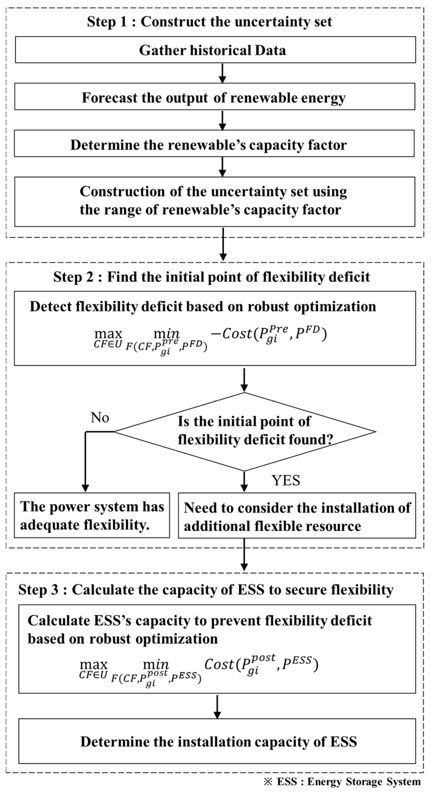
2.2.1. Searching for the Initial Point of Flexibility Deficit within the Uncertainty Set

Objective Function

The objective function consists of the sum of the cost of the generation and penalty (e.g., load shedding and curtailment). The generation cost is considered based on a quadratic function of the fuel cost of the thermal units, because renewable energy generation has a comparatively low cost. The penalty cost is expressed based on the amount of flexibility deficit multiplied by its cost coefficient and is a sufficiently large positive constant because it is related to a flexibility deficit causing load shedding and curtailment to balance supply and demand. The objective function can be formulated as follows:
max C F U min y Ω ( C F , P g i p r e ) C o s t ( P g i p r e , P F D )
C o s t ( P g i p r e , P F D ) = g i N G ( α g i + β g i · P g i p r e + γ g i · ( P g i p r e ) 2 ) + c F D · P F D    i N G
where N G denotes the number of generators and α g i , β g i , and γ g i denote the cost coefficients of the ith thermal unit; c F D denotes the cost coefficient of a flexibility deficit; and P g i p r e and P F D denote the output of the ith thermal unit and the total amount of flexibility deficit, respectively.
An increase in the capacity factor affects the decrease in total net load and generation, which can decrease the total cost of power generation if the power system has sufficient flexible resources to take action against the variation in renewable energy. However, from the perspective of a flexibility deficit, the value of the objective function increases owing to the penalty cost. Thus, just before the point of flexibility deficit is reached, Equation (4) reaches its smallest value. The use of a negative sign in Equation (4) changes it to the largest value just before the point when a flexibility deficit occurs. This allows searching for the initial point of the flexibility deficit within an uncertainty set, because robust optimization considers the worst-case scenario within the set. Accordingly, using this objective function, the initial point of the flexibility deficit can be found, and whether the power system has sufficient flexible resources to ensure nonnegative flexibility within the uncertainty set can be confirmed before determining whether to invest in flexible resources. In this step, it is assumed that the power system has only ramp rates as flexible resources.

Constraints

The constraints are composed of 3 parts: (i) conventional generators and renewable energy output, (ii) power balance, and (iii) power system flexibility.
(i) Output of Conventional Generators and Renewable Energy Sources
The output of a conventional generator is determined within the range of minimum and maximum limits of the generator. In addition, the output of renewable energy changes in accordance with the capacity factor:
P g i p r e _ P g i p r e P g i p r e ¯    i N G
P r e , i p r e = C F × P r e , i r a t e d    i N R E
where P g i p r e _ and P g i p r e ¯ are the minimum and maximum outputs of the ith generator, respectively, and P r e , i r a t e d is the rated capacity of renewable energy sources.
(ii) Power Balance
The output of a conventional generator is determined within the range of minimum and maximum limits of the generator. In addition, the output of renewable energy changes in accordance with the capacity factor:
i N d P d i = i N G P g i p r e + i N R E P r e , i p r e + P F D
where P d i is the demand at load i. The left-hand side of Equation (7) indicates the total load, and the right-hand side indicates the total sum of power generation and the amount of flexibility deficit. When a flexibility deficit occurs owing to a lack of flexible resources, it can meet the power balance using P F D p r e .
(iii) Power System Flexibility
In [14], the method for securing power system flexibility is intended to keep the amount of available flexibility higher than the flexibility requirement. The available flexibility means the total amount of flexible resources required to respond to variations in the net load, and the flexibility requirement means the net load ramp. Eventually, to ensure flexibility, the power system should secure flexible resources in advance to prevent a flexibility deficit. In this paper, the flexibility requirement is a variation in renewable energy by applying its variability rate, and the available flexibility simply considers the total sum of the ramp rates, which can be expressed as follows:
Δ P r e , i p r e = P r e , i p r e × V a r i a b i l i t y R a t e    i N R E .
R g i p r e u p = M i n ( R a m p r a t e g i u p , P g i p r e ¯ P g i p r e )    i N G
R g i p r e d o w n = M i n ( R a m p r a t e g i d o w n , P g i p r e P g i p r e _ )    i N G
i N R E Δ P r e , i p r e i N G R g i p r e u p P F D
  i N R E Δ P r e , i p r e i N G R g i p r e d o w n P F D
where Δ P r e , i p r e is the ramp of renewable energy as the requirement of flexibility, and R g i p r e u p and R g i p r e d o w n are the upward and downward reserves, respectively, at the ith generator that are able to offer active power over a certain period of time depending on the ramp rate. Therefore, Equation (8) defines the flexibility requirement, and Equations (9) and (10) are the available flexibility at the ith generator, enabling an increase and decrease in output within the time interval. Equations (11) and (12) determine the amount of flexibility deficit. When the left-hand side is lower than zero, the flexible resources are adequate to ensure nonnegative flexibility. However, when the left-hand side is higher than zero, the power system has inadequate flexible resources to respond to the net load ramp.

2.2.2. Determining the Capacity of Flexible Resources to Ensure Nonnegative Flexibility

Objective Function

The objective function is composed of the sum of the cost of thermal generation and ESS installation. The cost of thermal generation is the same as the quadratic equation given above. The cost of ESS installation can be expressed based on its capacity multiplied by its cost coefficient. The magnitude of the cost coefficient is sufficiently large to minimize the required capacity of the ESS to prevent a flexibility deficit from the net load ramp. The objective function is formulated as follows:
max C F U min y Ω ( C F , P g i p o s t ) C o s t ( P g i p o s t , P E S S )
C o s t ( P g i p o s t , P E S S ) = g i N G ( α g i + β g i · P g i p o s t + γ g i · ( P g i p o s t ) 2 ) + c E S S · P E S S    i N G
where c E S S denotes the cost efficiency of installing the ESS, and P g i p o s t and P E S S denote the output of the ith thermal unit and the amount of the required ESS, respectively.
The cost of charging and discharging an ESS is neglected in the objective function because it is much lower than that of installing the ESS. In addition, the cost of installation may considerably affect the value of the objective function compared with charging and discharging the ESS. When the initial flexibility deficit is found in the previous stage, installing an ESS is needed to secure sufficient flexible resources. In this stage, the minimum capacity of the ESS needed to ensure nonnegative flexibility within the uncertainty set is shown.

Constraints

The constraints consist of four parts: (i) conventional generators and renewable energy output, (ii) power balance, (iii) power system flexibility, and (iv) an ESS.
(i) Energy Output of Conventional Generators and Renewable Energy Sources
The constraints on the output of a conventional generator and renewable energy sources are the same as in Equations (5) and (6), which can be expressed as follows:
P g i p o s t _ P g i p o s t P g i p o s t ¯    i N G
P r e , i p r e = C F × P r e , i r a t e d    i N R E
(ii) Power Balance
The constraint of a power balance is almost the same as in Equation (7), except that the flexibility deficit is substituted with the charge and discharge of the ESS, which can be represented as follows:
i N d P d i = i N G P g i p r e + i N R E P r e , i p r e + ( P e s s d i s P e s s c h a )
where P e s s d i s and P e s s c h a are the magnitude of discharging and charging the ESS to protect the flexibility deficit within the uncertainty, respectively. Here, P e s s d i s can respond to an upward flexibility deficit, and P e s s c h a is able to cope with a downward flexibility deficit. Therefore, the power system is reinforced by the ESS, avoiding a flexibility deficit.
(iii) Power System Flexibility
The constraint of the power system flexibility is almost the same as in Equations (8)–(12) except for an additional part, the charging and discharging ESS in Equations (21) and (22), which is formulated as follows:
Δ P r e , i p o s t = P r e , i p o s t × V a r i a b i l i t y R a t e    i N R E .
R g i p r e u p = M i n ( R a m p r a t e g i u p , P g i p o s t ¯ P g i p o s t )    i N G
R g i p r e d o w n = M i n ( R a m p r a t e g i d o w n , P g i p o s t P g i p o s t _ )    i N G
i N R E Δ P r e , i p o s t ( i N G R g i p o s t u p + P e s s d i s ) P F l e x
i N R E Δ P r e , i p o s t ( i N G R g i p o s t d o w n + P e s s c h a ) P F l e x
where P F l e x denotes the additional required flexibility. If P F l e x = 0, minimum flexibility is ensured within the uncertainty set by installing the minimum ESS. In this paper, P F l e x is set to zero because the minimum capacity of the ESS is calculated to secure adequate flexible resources with the uncertainty set.
(iv) Energy Storage System (ESS)
When a net load ramp caused by variability in renewable energy sources occurs, it may be necessary to supply or absorb electricity. Thus, the capacity of an ESS can be composed of the sum of the charge and discharge required to avoid a flexibility deficit unless sufficient ramp rates exist as a flexible resource in the previous stage, which can be expressed as follows:
P E S S = η e s s c h a · P e s s c h a + 1 η e s s d i s · P e s s c h a
0 P e s s c h a , P e s s d i s
where η e s s c h a and η e s s d i s are the efficiency of the charging and discharging ESS. Indeed, losses occur when the ESS is charging and discharging. To calculate the capacity of the ESS, the efficiency should be considered in the problem.

2.3. Description of the Proposed Method

This paper presents a counterplan to prevent a flexibility deficit with flexible resources including ramp rates and ESS, which is coordinated with robust optimization. The process is composed of three parts: (i) constructing the uncertainty set with the capacity factor of renewable energy, (ii) searching the initial point of the flexibility deficit within the uncertainty, and (iii) calculating the capacity of the ESS to secure flexibility within the uncertainty set. First, based on historical or predicted data about renewable energy sources, the uncertainty set of the capacity factor is constructed. Whether the initial point of the flexibility deficit is found by the robust optimization within the uncertainty set is then examined. If an initial point exists, the power system needs additional flexible resources to secure flexibility under high-level penetration of renewable energy against the net load ramp. After searching for the initial point, based on the robust optimization, how much ESS capacity is needed to ensure nonnegative flexibility from the net load ramp can be calculated. The proposed method is shown in Figure 2.

3. Simulation and Results

This section describes verification of the proposed method using a power system in the Republic of Korea. After determining the interval of the capacity factor as the uncertainty set, the system checks whether a flexibility deficit occurs or whether sufficient ramp rates exist to provide flexible resources, which is considered a ramp rate in this step. Next, the capacity of flexible resources required by the power system to prevent a flexibility deficit is determined. This study was implemented using MATLAB 2017a, YALMIP20180612 as the optimization model language [38], and CPLEX 12.7 as the optimization solver. YALMIP can solve the robust optimization problem based on MATLAB with a variable solver including CPLEX and GROUBI.

3.1. Data Description

This study was conducted on a power system in the Republic of Korea. The offline generators were not considered because the flexibility was provided using in-service generators within a short period of time. There are 143 conventional generators in service, with a total capacity of approximately 93.175 GW. The system is composed of a gas turbine, hydropower, coal-fuel, liquefied natural gas (LNG), and nuclear units. The generation cost depends on the cost coefficient of the generators. Table 1 shows the generator data including number of generators, average ramp rates, maximum and minimum outputs, and cost coefficients.
According to [1,2], the total capacity of renewable energy will be from 11.3 GW in 2017 to 58.5 GW in 2030, when solar and wind power will be the main renewable resources and make up more than 88% of the total capacity of renewable energy. In this study, the output of renewable energy source is related to the capacity factor, which is considered an uncertainty set by assuming a range of 20–40%. In addition, the peak load predicted for 2030 is considered and is predicted to be 100.5 GW, assuming that the load will increase by an average of 1.3% per year [2].

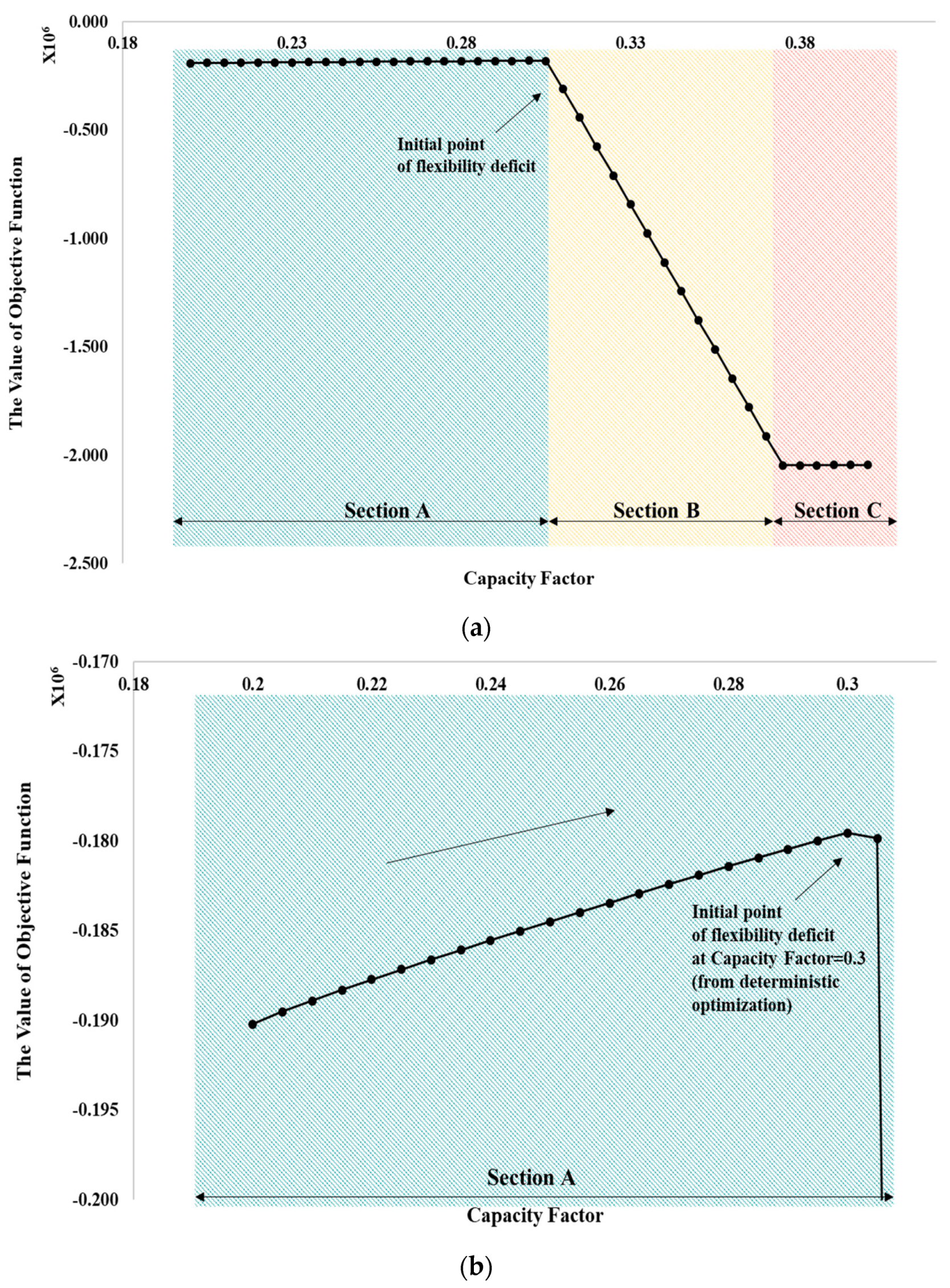
3.2. Searching for the Initial Point of Flexibility Deficit with Robust Optimization

The proposed robust optimization in step 2 is applied to find the initial point of the flexibility deficit within the uncertainty set. In this simulation, for a flexible resource, only the ramp rates are considered by assuming that there are no other flexible resources, such as an ESS. The result is shown in Table 2. The initial point of the flexibility deficit occurs at a capacity factor of 0.3051, which means the power system requires additional flexible resources such as ramp rates, an ESS, and the demand response to prevent a flexibility deficit. In addition, it has the highest value within the range of the capacity factor because the objective function has a negative sign.
The above results were analyzed in more detail by increasing the capacity factor by 0.005, from 0.2 to 0.4, using a deterministic method, which is represented in Figure 3 and Figure 4. Figure 3a is divided into three parts: a section ensuring a flexibility deficit (A), a section with an increase in the flexibility deficit (B), and a section with a nearly uniform flexibility deficit (C). Unless a flexibility deficit exists, the more the capacity factor of renewable energy increases, the greater the total decrease in power generation, which can affect the cost of power generation or the absolute value of the objective function. So, in section A, the value of the objective function gradually increases by increasing the capacity factor of renewable energy, since the objective function has a negative sign, shown in Figure 3b. However, after the initial point of the flexibility deficit, the absolute value of the objective function can increase, owing to the penalty of the deficit. Thus, section A has a higher cost than sections B and C, because not only is there no flexibility deficit, but the objective function also has a negative sign. The initial point of the flexibility deficit is also located at the capacity factor of renewable energy = 0.3 between section A and section B from the deterministic approach. Through this result, the robust and deterministic approach is almost the same.
Owing to the flexibility deficit, sections B and C need additional flexible resources to respond to the net load ramp. Section B shows an increase in the flexibility deficit because of insufficient ramp rates as flexible resources. Although section C is also an interval with a flexibility deficit, its interval seldom has an increase in flexibility deficit owing to the increase in ramp rates caused by a reduction in power generation. An increase in the generation of renewables can increase variation and uncertainty, while it can affect the decrease in net load and total power generation and the increase in ramp rates.

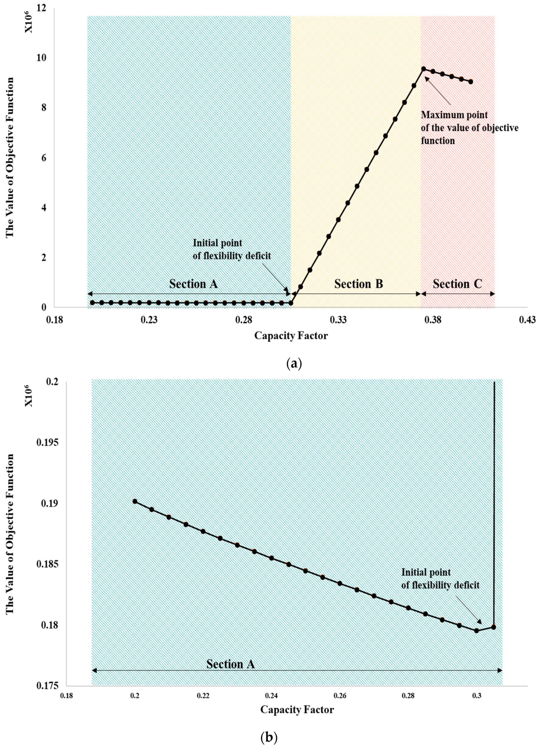
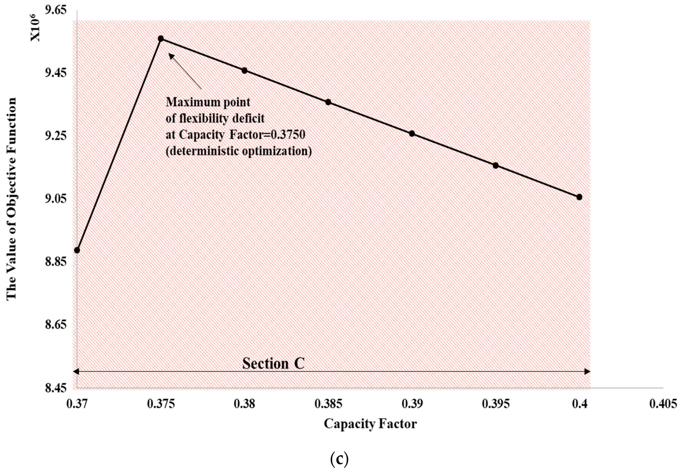
3.3. Determining the Capacity of Eenergy Storage System(ESS) to Ensure Nonnegative Flexibility

The capacity of an ESS to ensure nonnegative flexibility through the proposed robust optimization applied in step 3 was determined. The results are compared between deterministic and robust optimizations, shown in Table 3. Using a deterministic approach, the results show that the cost is small when the capacity factor is 0.2. The cost of the capacity factor, 0.4, is about 42.06 times higher than that of the capacity factor, 0.2, which occurs from the ESS installation to ensure nonnegative flexibility. Indeed, when the capacity factor is 0.4, many more flexible resources are needed than with a capacity factor of 0.2. It is reasonable that there is a need for flexible resources caused by an increase in the variation of renewable energy when the capacity factor is higher. Reviewing the results of robust optimization, when the capacity factor is 0.3749 within the uncertainty set, the necessary capacity of the ESS has a maximum value of 1875.7 MW. This means the system requires the largest capacity of the ESS installation within the uncertainty set.
To analyze this result in detail, the previous deterministic approach is used, which is a method for increasing the capacity factor from 0.2 to 0.4 by steps of 0.05. The results are shown in Figure 5. Within the range of the capacity factor, the results based on a deterministic approach show that the value of the objective function is the smallest when the capacity factor is 0.300 and the highest when the capacity factor is 0.375, as shown in Figure 5a. In section A, the cost of power generation decreases through an increase in the capacity factor of renewable energy and a decrease in total generation and net load, shown in Figure 5b. The point at a capacity factor of 0.300 is the smallest value of the objective function and is located near the initial point of the flexibility deficit. In section C, the value of the objective function gradually decreases because the ramp rates increase by reducing the power generation. The maximum point of the value of objective function is placed at a capacity factor of renewable energy = 0.375 between sections B and C from the deterministic approach. Also, the capacity factor is almost the same as the result of robust optimization. Sections B and C both require additional flexible resources to prevent a flexibility deficit. However, section B increases the flexibility deficit and section C no longer increases the flexibility deficit by increasing the capacity factor of renewable energy. Due to this fact, in section C, the value of the objective function decreases by increasing the capacity factor of renewable energy, shown in Figure 5c. The details of this are introduced in Figure 6.
In section A, the total sum of ramp rates increases owing to a decrease in the net load through an increase in the renewable energy output. In section B, the total sum of ramp rates gradually decreases because of a decline in the number of generators required to maintain supply and demand. In addition, in section C, the total sum of ramp rates increases again because the number of generators out of service no longer increases. This may be why the necessary capacity of an ESS is not the highest at the maximum capacity factor despite the increase in variability and uncertainty from renewable energy.

4. Conclusions

A deterministic optimization cannot consider uncertainty, which can undermine the reliability of the solution owing to an inability to reflect the uncertainty. In previous studies using deterministic optimization and stochastic programming, in order to consider uncertainty such as that found with renewable energy, it was necessary to make scenarios. For example, all capacity factors of renewable energy constructed by a planner are reviewed to decide how the system will be reinforced for stable operation despite variation and uncertainty, which may require much effort to do. However, robust optimization does not require creating scenarios or using much effort because it needs the uncertainty set. Therefore, it is proper to use robust optimization to include uncertainty. In actuality, in power system planning and operation, because it is extremely difficult to take into account all possible scenarios, it is reasonable to prepare a countermeasure for the worst case. Therefore, robust optimization is a suitable model in power system planning and operation.
This paper presents a robust optimization model to secure flexible resources and prevent the occurrence of a flexibility deficit from the variability and uncertainty of renewable energy. This model considers the capacity factor of renewable energy as the uncertainty set and is divided into two steps: (i) searching for the initial point of the flexibility deficit and (ii) determining the capacity of the ESS to ensure nonnegative flexibility. In the first step, it is determined whether a flexibility deficit point occurs within the interval of the capacity factor when only considering ramp rates as flexible resources. This step takes place before determining whether to invest in flexible resources. In the next step, the necessary capacity of the ESS is calculated, which can ensure nonnegative flexibility within the uncertainty set. Through this study, the results of the worst case using a deterministic approach and robust optimization are similar. Indeed, searching the worst case using a deterministic approach may require many things, from making to studying scenarios, but robust optimization may be able to reduce the effort of considering the worst case without creating scenarios.
Future work will include more detailed modeling, including power flow limits of transmission lines and unit commitment to improve the quality of the solution. It will also be necessary to contain realistic conditions to guarantee a solution.

Author Contributions

J.J. conceived and designed the research methodology, performed the system simulations, and wrote this paper. B.L. supervised the research, improved the system simulation, and made suggestions regarding this research. The other authors discussed and contributed to the writing of the paper.

Funding

This research was supported by the Korea Electric Power Corporation (grant number: R17XA05-4) and the Human Resource Program in Energy Technology of the Korea Institute of Energy Technology Evaluation and Planning (KETEP) granted financial resource from the Ministry of Trade, Industry & Energy, Republic of Korea (No. 20174030201820).

Conflicts of Interest

No conflicts of interest relevant to this article are reported.

References

  1. The Ministry of Trade, Industry and Energy. New and Renewable Energy 3020 Implementation Plan; The Ministry of Trade, Industry and Energy: Sejong-si, Korea, 2017. (In Korean)
  2. The Ministry of Trade, Industry and Energy. The 8th Basic Plan for Long-Term Electricity Supply and Demand (2017–2031); The Ministry of Trade, Industry and Energy: Sejong-si, Korea, 2017. (In Korean)
  3. Stram, B.N. Key challenges to expanding renewable energy. Energy Policy 2016, 96, 728–734. [Google Scholar] [CrossRef]
  4. Kunz, H.; Hagens, N.; Balogh, S. The Influence of Output Variability from Renewable Electricity Generation on Net Energy Calculations. Energies 2014, 7, 150–172. [Google Scholar] [CrossRef] [Green Version]
  5. Haas, J.; Cebulla, F.; Cao, K.; Nowak, W.; Palma-Behnke, R.; Rahmann, C.; Mancarella, P. Challenges and trends of energy storage expansion planning for flexibility provision in low-carbon power systems—A review. Renew. Sustain. Energy Rev. 2017, 80, 603–619. [Google Scholar] [CrossRef]
  6. Bae, M.; Lee, H.; Lee, B. An Approach to Improve the Penetration of Sustainable Energy Using Optimal Transformer Tap Control. Sustainability 2017, 9, 1536. [Google Scholar] [Green Version]
  7. Liu, Z.; Chen, Y.; Luo, Y.; Zhao, G.; Jin, X. Optimized Planning of Power Source Capacity in Microgrid, Considering Combinations of Energy Storage Devices. Appl. Sci. 2016, 6, 416. [Google Scholar] [CrossRef]
  8. Shigenobu, R.; Noorzad, A.; Muarapaz, C.; Yona, A.; Senjyu, T. Optimal Operation and Management of Smart Grid System with LPC and BESS in Fault Conditions. Sustainability 2016, 8, 1282. [Google Scholar] [CrossRef]
  9. Tuohy, A. Flexibility in Transmission and Resource Planning; EPRI: Palo Alto, CA, USA, 2014. [Google Scholar]
  10. EPRI. Metrics for Quantifying Flexibility in Power System Planning; EPRI: Palo Alto, CA, USA, 2014. [Google Scholar]
  11. Cochran, J.; Miller, M.; Zinaman, O.; Milligan, M.; Arent, D.; Palmintier, B.; O’Malley, M.; Mueller, S.; Lannoye, E.; Tuohy, A.; et al. Flexibility in 21st Century Power Systems; National Renewable Energy Lab. (NREL): Golden, CO, USA, 2014. [Google Scholar]
  12. Danish Energy Agency. Flexiblity in the Power System—Danish and European Experience, 2015. Available online: https://ens.dk/sites/ens.dk/files/Globalcooperation/flexibility_in_the_power_system_v23-lri.pdf (accessed on 9 November 2018).
  13. Poncela, M.; Purvins, A.; Chondrogiannis, S. Pan-European Analysis on Power System Flexibility. Energies 2018, 11, 1765. [Google Scholar] [CrossRef]
  14. Lannoye, E.; Daly, P.; Tuohy, A.; Flynn, D.; O’Malley, M. Assessing Power System Flexibility for Variable Renewable Integration: A Flexibility Metric for Long-Term System Planning. CIGRE Sci. Eng. J. 2015, 3, 26–39. [Google Scholar]
  15. California ISO. Final Flexible Capacity Needs Assessment for 2019, 2018. Available online: http://www.caiso.com/informed/Pages/StakeholderProcesses/FlexibleCapacityNeedsAssessmentProcess.aspx (accessed on 9 November 2018).
  16. California ISO. Flexible Ramping Product Uncertainty Calculation and Implementation Issues, 2018. Available online: https://www.caiso.com/Documents/FlexibleRampingProductUncertaintyCalculationImplementationIssues.pdf (accessed on 9 November 2018).
  17. Rodrigues, E.M.G.; Godina, R.; Santos, S.F.; Bizuayehu, A.W.; Contreras, J.; Catalão, J.P.S. Energy storage systems supporting increased penetration of renewables in islanded systems. Energy 2014, 75, 265–280. [Google Scholar] [CrossRef]
  18. Denholm, P. Energy storage to reduce renewable energy curtailment. In Proceedings of the 2012 IEEE Power and Energy Society General Meeting, San Diego, CA, USA, 22–26 July 2012; pp. 1–4. [Google Scholar]
  19. Jirutitijaroen, P.; Singh, C. Reliability Constrained Multi-Area Adequacy Planning Using Stochastic Programming with Sample-Average Approximations. IEEE Trans. Power Syst. 2008, 23, 504–513. [Google Scholar] [CrossRef]
  20. Hajipour, E.; Bozorg, M.; Fotuhi-Firuzabad, M. Stochastic Capacity Expansion Planning of Remote Microgrids with Wind Farms and Energy Storage. IEEE Trans. Sustain. Energy 2015, 6, 491–498. [Google Scholar] [CrossRef]
  21. Zhan, Y.; Zheng, Q.P.; Wang, J.; Pinson, P. Generation Expansion Planning with Large Amounts of Wind Power via Decision-Dependent Stochastic Programming. IEEE Trans. Power Syst. 2017, 32, 3015–3026. [Google Scholar] [CrossRef]
  22. Alharbi, H.; Bhattacharya, K. Stochastic Optimal Planning of Battery Energy Storage Systems for Isolated Microgrids. IEEE Trans. Sustain. Energy 2018, 9, 211–227. [Google Scholar] [CrossRef]
  23. Ruiz, C.; Conejo, A.J. Robust transmission expansion planning. Eur. J. Oper. Res. 2015, 242, 390–401. [Google Scholar] [CrossRef]
  24. Dehghan, S.; Amjady, N. Robust Transmission and Energy Storage Expansion Planning in Wind Farm-Integrated Power Systems Considering Transmission Switching. IEEE Trans. Sustain. Energy 2016, 7, 765–774. [Google Scholar] [CrossRef]
  25. Liu, D.; Shang, C.; Cheng, H. A two-stage robust optimization for coordinated planning of generation and energy storage systems. In Proceedings of the 2017 IEEE Conference on Energy Internet and Energy System Integration (EI2), Beijing, China, 26–28 November 2017; pp. 1–5. [Google Scholar]
  26. Thatte, A.A.; Sun, X.A.; Xie, L. Robust Optimization Based Economic Dispatch for Managing System Ramp Requirement. In Proceedings of the 2014 47th Hawaii International Conference on System Sciences, Waikoloa, HI, USA, 6–9 January 2014; pp. 2344–2352. [Google Scholar]
  27. Ampatzis, M.; Nguyen, P.H.; Kamphuis, I.R.; van Zwam, A. Robust optimisation for deciding on real-time flexibility of storage-integrated photovoltaic units controlled by intelligent software agents. IET Renew. Power Gener. 2017, 11, 1527–1533. [Google Scholar] [CrossRef]
  28. Lorca, A.; Sun, X.A. Adaptive Robust Optimization with Dynamic Uncertainty Sets for Multi-Period Economic Dispatch Under Significant Wind. IEEE Trans. Power Syst. 2015, 30, 1702–1713. [Google Scholar] [CrossRef]
  29. Yi, J.; Lyons, P.F.; Davison, P.J.; Wang, P.; Taylor, P.C. Robust Scheduling Scheme for Energy Storage to Facilitate High Penetration of Renewables. IEEE Trans. Sustain. Energy 2016, 7, 797–807. [Google Scholar] [CrossRef]
  30. Kim, J.; Choi, Y.; Ryu, S.; Kim, H. Robust Operation of Energy Storage System with Uncertain Load Profiles. Energies 2017, 10, 416. [Google Scholar] [CrossRef]
  31. Ben-Tal, A.; El Ghaoui, L.; Nemirovski, A. Robust Optimization; Princeton University Press: Princeton, NJ, USA, 2009; Volume 28. [Google Scholar]
  32. Ben-Tal, A.; Nemirovski, A. Robust optimization—Methodology and applications. Math. Program. 2002, 92, 453–480. [Google Scholar] [CrossRef]
  33. Steuben, J.C.; Turner, C.J. Robust optimization of mixed-integer problems using NURBs-based metamodels. J. Comput. Inf. Sci. Eng. 2012, 12, 041010. [Google Scholar] [CrossRef]
  34. Bertsimas, D.; Sim, M. The price of robustness. Oper. Res. 2004, 52, 35–53. [Google Scholar] [CrossRef]
  35. Bertsimas, D.; Dunning, I.; Lubin, M. Reformulation versus cutting-planes for robust optimization. Comput. Manag. Sci. 2016, 13, 195–217. [Google Scholar] [CrossRef]
  36. Yuan, Y.; Li, Z.; Huang, B. Robust optimization under correlated uncertainty: Formulations and computational study. Comput. Chem. Eng. 2016, 85, 58–71. [Google Scholar] [CrossRef]
  37. Bertsimas, D.; Brown, D.B.; Caramanis, C. Theory and Applications of Robust Optimization. SIAM Rev. 2011, 53, 464–501. [Google Scholar] [CrossRef] [Green Version]
  38. Löfberg, J. Automatic robust convex programming. Optim. Methods Softw. 2012, 27, 115–129. [Google Scholar] [CrossRef] [Green Version]
Figure 1. Process of constructing the uncertainty set.
Sustainability 10 04159 g001
Figure 2. Proposed method.
Sustainability 10 04159 g002
Figure 3. Results of deterministic optimization per 0.005 increase in capacity factor for step 2: values of objective function (a) within the interval of the capacity factor and (b) of section A.
Sustainability 10 04159 g003
Figure 4. Results of deterministic optimization per 0.005 increase of capacity factor for step 2.
Sustainability 10 04159 g004
Figure 5. Results of deterministic optimization per 0.005 increase in capacity factor for step 3: values of objective function (a) within the interval of the capacity factor, (b) of section A, and (c) of section C.
Sustainability 10 04159 g005aSustainability 10 04159 g005b
Figure 6. Total capacity of flexible resources by capacity factor.
Sustainability 10 04159 g006
Table 1. Data of in-service generators. Liquefied natural gas (LNG)
Total NumberRamp Rate (MW/h)Pmin
(MW)
Pmax
(MW)
ai
(₩/h)
bi
(₩/MWh)
ci
(₩/MW2h)
Gas turbine1826.669259.500627.044370.51581.291710.000976
Hydro22119.15490.227280.72716.543941.706690.006959
Coal-fuel6015.702357.353649.480164.34391.825540.000317
LNG2525.564230.800614.13994.97751.437320.000270
Nuclear181.766973.1111188.333473.35571.695360.000296
Table 2. Initial point of flexibility deficit.
Capacity FactorValue of Objective Function
Robust0.3051−179,890
Table 3. Comparison between deterministic and robust results.
Capacity FactorValue of Objective FunctionInstallation of ESS (MW)
Deterministic0.2000215,2790
Deterministic0.40009,056,1401777.4
Robust0.37499,545,5561875.7

