Decision-Making Method based on Mixed Integer Linear Programming and Rough Set: A Case Study of Diesel Engine Quality and Assembly Clearance Data

Abstract

The purpose of this paper is to establish a decision-making system for assembly clearance parameters and machine quality level by analyzing the data of assembly clearance parameters of diesel engine. Accordingly, we present an extension of the rough set theory based on mixed-integer linear programming (MILP) for rough set-based classification (MILP-FRST). Traditional rough set theory has two shortcomings. First, it is sensitive to noise data, resulting in a low accuracy of decision systems based on rough sets. Second, in the classification problem based on rough sets, the attributes cannot be automatically determined. MILP-FRST has the advantages of MILP in resisting noisy data and has the ability to select attributes flexibly and automatically. In order to prove the validity and advantages of the proposed model, we used the machine quality data and assembly clearance data of 29 diesel engines of a certain type to validate the proposed model. Experiments show that the proposed decision-making method based on MILP-FRST model can accurately determine the quality level of the whole machine according to the assembly clearance parameters.

1. Introduction

Diesel engine is the power core of the ship. In the manufacturing process of the diesel engine, the assembly quality affects the performance indexes of the diesel engine, which is an important factor to measure the quality of the whole engine. Previous studies on the relationship between assembly clearance and machine quality have mainly focused on the mechanical principle, while the data mining method is still less used to mine the relationship between assembly clearance and machine quality. With the development of data mining technology and the accumulation of a large number of raw data, it is possible to apply data mining methods to solve this problem.

With the development of computers and the internet, the amount of data is increasing. Data always contain noise; therefore, it is necessary to handle noisy data to obtain accurate results. Some researchers have put forward methods to address this issue. Among these methods, the two classic methods are fuzzy set [1] and evidence theory [2]. However, these methods sometimes require additional information or prior knowledge, such as fuzzy membership functions, basic probability assignment functions and statistical probability distributions, which are not always easy to obtain.

Rough set theory provides a new way to address vagueness and uncertainty [3]. The core concept of rough set theory is to deduce imprecise data, or to find the correlation between different data by representing the given finite set as an upper approximation set or a lower approximation set.

Despite the advantages of rough set theory, some challenges need to be overcome in practical applications. These problems can be classified into two categories: (1) There are certain limitations of a rough set in practical applications. Many extension and correction theories to the classical rough set have been developed. For example, a model integrating distance and partition distance with a rough set on the basis of a rough set based on a similarity relation was proposed [4]. This model also provided a new understanding of the classification criteria of rough set equivalence classes. Φ-Rough set, another extension of the rough set theory based on the similarity relation, was proposed [5]. Φ-Rough set replaces the indiscernibility relation of the crisp rough set theory by the notion of the Φ-approximate equivalence relation. Use of dynamic probabilistic rough sets with incomplete data addressed the challenge of processing such dynamic and incomplete data [6]. Based on a three-way classification of attributes into the pair-wise disjoint sets of core, marginal, and non-useful attributes, the relationships between the corresponding classes of classification-based and class-specific attributes were examined [7]. (2) A rough set is sensitive to noisy data. The accuracy of a decision-making model based on a rough set is low when applied to the analysis of datasets containing noisy data [8]. To strengthen its ability to resist noisy data, the variable precision rough set (in short, VPRS) was proposed [9]. VPRS has been applied in several fields, such as data mining [10], decision systems [11], and expert systems [12], and provides satisfactory results. Similarly, knowledge reduction is an important research direction of VPRS. However, the related methods and theories are not mature. The most popular study based on VPRS is attribute reduction. In addition, variable precision threshold beta is usually determined by experts. Hence, some researchers have proposed the selection method of beta, which can reduce the difficulty of beta determination due to a lack of prior knowledge [13,14]. Zavareh M. and Maggioni V. proposes an approach to analyze water quality data that is based on rough set theory [15]. Bo C. studies multigranulation neutrosophic rough sets (MNRSs) and their applications in multi-attribute group decision-making [16]. Akram M., Ali G. and Alsheh N. O. introduce notions of soft rough m-polar fuzzy sets and m-polar fuzzy soft rough sets as novel hybrid models for soft computing, and investigate some of their fundamental properties [17]. Jia X. et al. propose an optimization representation of decision-theoretic rough set model. An optimization problem is proposed by considering the minimization of the decision cost [18]. Cao T. et al. discusses the use of parallel computation to obtain rough set approximations from large-scale information systems where missing data exist in both condition and decision attributes [19].

The linear programming method is a classical mathematical method, and its principle is to solve a series of linear constraint equations or inequalities on the premise of satisfying the method of solving linear functions of extreme objectives. Though its mathematical model is simple, it is widely used in various fields, such as location problems, route planning problems, manufacturing problems, marketing problems, and resource allocation problems. Application of the linear programming method can provide an effective and feasible decision-making basis for the aforementioned problems.

The linear programming problem (LP) is a problem of solving the maximum or minimum value of a linear function under a set of linear equality and inequality constraints [20]. The general linear programming model is composed of the following elements parameters and variables, objective functions, and constraint conditions.

There has been much research on optimization problems based on linear programming theory, such as the theory of linear programming and establishment of a mathematical model [21], as well as the combination of practical production, and enterprise and establishment of a linear programming model to solve the problem of allocating enterprise production resources [22]. Linear programming methods have also been used to optimize input–output models, and to establish a multi-objective linear programming model to maximize economic benefits and to minimize resource utilization [23]. One of the most important application fields of linear programming are location problems. A mixed integer linear programming model has been built to select the location of renewable energy facilities [24], and to study a multi-stage facility location problem [25]. To solve the vehicle routing problem of a distribution center, a two-stage solution was proposed.

One of the preprocessing methods of noisy data is regression. Hence, it is obvious that the linear programming model has a strong ability to resist noisy data, and designing a decision-making model based on rough set achieves the ideal accuracy. The integration of the rough set with the linear programming model will not only improve the inadequacies of the rough set, but will also make the decision-making model reach optimal accuracy, theoretically. There are a few studies on the integration of the rough set and linear programming model so far. Zhang et al. proposed a multi-objective linear programming method based on the rough set, to develop a classification for data mining. Based on their model, an improved model to predict hot spots of protein interactions was proposed [26]. However, among all of the above studies, the rough set was only used to reduce the attribute set. Because nonlinear models are considered to be the only way to describe the rough set, there are no studies on the application of linear programming methods to optimize decision-making models based on the rough set.

The biggest weakness of the decision model based on the rough set is its sensitivity to noisy data. VPRS only broadens the requirement of the upper and lower approximations in the definition, and the selection of precision often has strong subjectivity and lacks scientific evidence. VPRS can only be used as an auxiliary method to improve the resistance of the rough set model to noisy data, rather than the main method. Therefore, in this study, we extend the rough set theory via mixed-integer linear programming and we propose a model called the mixed-integer linear programming model for rough set-based classification with flexible attribute selection (in short, MILP-FRST). This model includes the advantages of MILP in resisting noisy data, and it has the ability to select attributes flexibly and automatically. MILP-FRST is able to divide the universe by attribute sets, calculate the lower approximation set under the condition of the presupposed variable precision and the minimum support number, and calculate the decision accuracy and screen out attributes. We set the maximum number of elements in the determination area as the objective function of the model. The processing of attribute selection, and partitioning of the attribute set for the universe are maximized by the objective function. During implementation, attributes that have a significant influence on the accuracy of the decision system will be selected, and the attribute set partition scheme is calculated to achieve the highest accuracy of the decision-making system. In addition, rough set models are often considered to be nonlinear. This paper first describes the related concepts and theories using linear models, which are an extension of rough set theory.

Next, we use the model to mine the correlation between the assembly clearance of diesel engine and the quality of the whole engine based on the dataset, which contains 28 attributes of the assembly clearance parameters and the whole machine quality of 29 diesel engines. Before applying the model, we carry out data pretreatment, and we screen out 15 principal components. These components cover the vast majority of information on the assembly clearance parameters of all diesel engines. Then, we input these data into the model. The experimental results verified the effectiveness and advantages of MILP-FRST.

The rest of the paper is organized as follows. In Section 2, we introduce the concept of the rough set and functional dependence. In Section 3, we build a mixed-integer linear programming model for rough set-based classification with flexible attribute selection. In Section 4, we use the clearance parameter data of 29 diesel engines and the quality data of the whole engine to verify the validity and accuracy of the model. Finally, in Section 5, conclusions are presented.

2. Rough Set Theory

2.1. Concepts and Definitions of Rough Sets

Consider a rough set based on an information system [27]: $IS=(I,A)$, where I is the universe; A is the attribute set. Both I and A are nonempty finite sets.

If the information system meets the conditions that $A=C\cup D\ne \varnothing$, this information system can be called a decision-making system $DS=(I,C\cup D)$, where C is the conditional attribute set, and D is the decisive attribute set.

Definition 1.

Indiscernibility relations [27]: In an information system $IS=(I,A)$, set B is a subset of the attribute set A, binary relation $IND\left(B\right)=\{(x,y)\in I\times I:\forall a\in B,a(x)=a(y)\}$ is the indiscernibility relation of IS, recorded as $IND\left(B\right)$, where x and y are elements of the universe; a is an attribute of the attribute set; and $a\left(x\right)$ is the value of the element x in attribute a.

Definition 2.

Equivalence class [27]: In an information system $IS=(I,A)$, set B is a subset of the attribute set A. The indiscernibility relation $IND\left(B\right)$ divides the universe I into several equivalence classes, where $I/IND(B)$ is the set of all equivalence classes, and ${[x]}_{IND\left(B\right)}$ is the equivalence class containing element x.

Definition 3.

Upper and lower approximation [27]: In an information system $IS=(I,A)$, set B is a subset of the attribute set A, and set X is a subset of the universe I:

$$\underset{\_}{B}X=\{i\in I|{[i]}_{IND(B)}\subseteq X\}$$

(1)

$$\overline{B}X=\{i\in I|{[i]}_{IND\left(B\right)}\cap X\ne \varnothing \}$$

(2)

where $\underset{\_}{B}X$ is the lower approximation; $\overline{B}X$ is the upper approximation.

Definition 4.

The accuracy and membership grade [27] are:

$$a_B=\frac{|\underset{\_}{B}X|}{|\overline{B}X|}$$

(3)

$${\rho }_B=1-a_B$$

(4)

where $a_B$ is the accuracy of rough set X, and ${\rho }_B$ is the membership grade of rough set X.

Definition 5.

The membership function [27] is:

$$\mu (x,X)=\frac{|{[x]}_B\cap X|}{|{[x]}_B|}$$

(5)

The membership function indicates the membership degree of element $x$ to the rough set X.

Definition 6.

The accuracy of the decision-making system [27] is:

$$\lambda =\frac{|{{\displaystyle \sum }}_{k=1}^{Kc}\underset{\_}{B}{X}_k|}{|I|}$$

(6)

Given that the strict definitions of the upper and lower approximations make the rough set sensitive to noisy data, the rough set cannot adapt well to all situations in practical applications. VPRS decreases the influence of missing data, incorrect data, and noisy data. In VPRS, an approximation variable precision $\beta$, which ranges from 0.5 to 1, represents the tolerance degree of the rough set to noisy data and incorrect data. $\beta$ can be defined as follows:

Definition 7.

$$\underset{\_}{B}{X}_{\beta }=\left\{i\in I|\frac{|{[i]}_{IND\left(B\right)}\cap X|}{|{[i]}_{IND\left(B\right)}|}\ge \beta \right\}$$

(7)

$$\overline{B}{X}_{\beta }=\left\{i\in I|\frac{|{[i]}_{IND\left(B\right)}\cap X|}{|{[i]}_{IND\left(B\right)}|}>1-\beta \right\}$$

(8)

where set B is a subset of the attribute set A; set X is a subset of the universe I; $\beta$ is the variable precision, which ranges from 0.5 to 1; $\underset{\_}{B}{X}_{\beta }$ is the lower approximation; and $\overline{B}{X}_{\beta }$ is the upper approximation.

Compared with the rough set, VPRS extends the range of the upper and lower approximation, thus restricting the sensitivity of the rough set model to noisy data.

The rough set uses the indiscernibility relation to classify equivalence classes, but it is unsuitable for numerical data, especially in the case of the application of big data and high accuracy. One way to overcome this difficulty is to use the similarity relation, so we can extend the rough set based on the similarity relation.

This extension essentially involves modifications of the two concepts of the rough set, the indiscernibility relation and equivalence class. The classical indiscernibility relation is more suitable for those descriptive attributes, while elements of an attribute set that satisfy the indiscernibility relation are divided into an equivalence class. However, when dealing with numeric data, the effect of this method will be considerably reduced. The rough set, based on the similarity relation extends the indiscernibility relation into a similarity relation, and the equivalence class classified by the indiscernibility relation is replaced by a similarity relation.

2.2. Rough Set and Functional Dependence

With the establishment of the rough set model with variable precision based on the similarity relation, the decision rules between approximately equivalence classes divided by the conditional attribute set and the approximate equivalence classes divided by decisive attribute set can be worked out. However, this is not enough to explain the correlation between the conditional attribute set and the decisive attribute set, and so, functional dependence is introduced. Although the rough set and functional dependence are two different fields, many concepts of functional dependence can be explained from the perspective of the rough set.

Definition 8.

Functional dependence, the complete dependence between universe I and attribute A, can be expressed as $C\to d$, where $C\subseteq A$, $d\in A$.

Definition 9.

Partial dependence, the partial dependence between universe I and attribute A, can be expressed as $C{\to }_{p}d$, where $C\subseteq A$, $d\in A$.

Inference 1.

Complete dependence of attribute set, any attribute $\in D$, $D\subseteq A$, $C\to d$ works. Accordingly, there is functional dependence between $C$ and $D$, and this relationship can be expressed as $C\to D$, where D is an attribute set.

Inference 2.

Partial dependence of attribute set, any attribute $\in D$, $D\subseteq A$, $C{\to }_{p}d$ works. Accordingly, there is partial functional dependence between $C$ and $D$, and this relationship can be expressed as $C{\to }_{p}D$, where D is an attribute set.

We now explain complete dependence and partial dependence from the perspective of the rough set. For a decision-making system based on the rough set, $\mathsf{\lambda }=1$ means that the decisive attribute set completely depends on the conditional attribute set, that is, there is complete dependence between the decisive attribute set and conditional attribute set. $0<\mathsf{\lambda }<1$ means that there are some factors that affect the decisive attribute set in addition to the conditional attribute set, that is, the decisive attribute set partially depends on the conditional attribute set, so the following inferences are introduced.

Inference 3.

Complete dependence in the rough set, in a decision-making system $DS=(U,C\cup D)$, only occurs when p $\mathsf{\lambda }=1$, and the complete dependence $C\to D$ comes into effect.

Inference 4.

Partial dependence in the rough set, in a decision-making system $DS=(U,C\cup D)$, $0<\mathsf{\lambda }<1$ indicates that there is partial dependence $C{\to }_{p}D$ between C and D, and the degree of partial dependence $p$ equals $\mathsf{\lambda }$.

After calculating the accuracy $\mathsf{\lambda }$ of the model, according to inference 3 and inference 4, if $\mathsf{\lambda }=1$, the decisive attribute set completely depends on the conditional attribute set. If $0<\mathsf{\lambda }<1$, the decisive attribute set partially depends on the conditional attribute set. In other words, there is a certain correlation between the conditional attribute set and the decisive attribute set, and $\mathsf{\lambda }$ can be used as a parameter to measure the degree of correlation.

This section proposes the rough set model with variable precision, based on the similarity relation and some inferences related to functional dependence. This method will not only dig out the correlation between the conditional attribute set and the decisive attribute set, but also use accuracy $\mathsf{\lambda }$ to measure the degree of correlation.

3. A Mixed-Integer Linear Programming Model for Rough Set-Based Classification with Flexible Attribute Selection

There is no doubt that the decision-making model based on the rough set has the congenital defect of the rough set; thus, adding variable precision to extend the rough set into the rough set with variable precision is necessary while building the model. Nevertheless, adding variable precision only broadens the range of the upper and lower approximations. The choice of precision is often subjective and lacks scientific basis. Above all, variable precision can only be used as an auxiliary method to improve the ability of the rough set model to reduce noisy data’s bad influence on accuracy.

In this study, we build a mixed-integer linear programming model for a rough set-based classification with flexible attribute selection, which has a strong ability to overcome the noise sensitivity of the rough set model. Meanwhile, this study explains the rough set model, which is often considered to be nonlinear, by using a linear model for the first time. It is also an extension of the rough set.

3.1. Rough Set Model Based on Mixed Integer Linear Programming

Applying mixed integer linear programming to optimize the rough set model is essentially explaining the definition that is related to the rough set by linear programming. The rough set in a linear model enables the maximum accuracy of dividing the equivalence class, so that the decision-making system based on the rough set can correctly determine the correlation between the conditional attribute set and the decisive attribute set.

This model focuses on the rough set based on the similarity relation, and compares the similarity of each attribute in the attribute set. Next, the elements that satisfy the similarity threshold on each attribute are selected as the elements to be divided into an approximate equivalence class.

This model can also screen out attributes in the attribute set and take the attribute makes a considerable impact in dividing the universe into the final attribute set to reduce the dimension of the attributes.

We use the following notations:

• I: Universe of elements.
• $k_c$: A set of approximate equivalence classes obtained by partitioning the conditional attribute set in the universe.
• $k_d$: A set of approximate equivalence classes obtained by partitioning the decisive attribute set in the universe.
• C: Conditional attribute set.
• D: Decisive attribute set.
• N: Minimum support number of the conditional attribute set.
• $\beta$: Variable precision.
• ${\alpha }_c$: Similarity threshold of the conditional attribute set.
• ${\alpha }_d$: Similarity threshold of the decisive attribute set.
• M: A large number.
• $X{c}_i$: Value of each element in each conditional attribute.
• $X{d}_i$: Value of each element in each decisive attribute.
• $\omega \_c_{ij}$: For any two elements i and j in universe I, if $\omega \_c_{ij}=1, i$ and $j$ are in the same approximate equivalence class divided by the conditional attribute set; otherwise, $\omega \_c_{ij}=0$.
• $s{l}_c$: $s{l}_c=1$ if attribute c will be selected as a new attribute set to divide universe; otherwise, $s{l}_c=0$.
• $q_{ik}$: For any element i in universe I and any approximate equivalence class k in the set of approximate equivalence classes divided by the conditional attribute set, $q_{ik}=1$ if i belongs to k; otherwise, $q_{ik}=0$.
• $s{s}_{ijc}$: Any two elements i and j in universe I and any attribute c in the conditional attribute set. $s{s}_{ijc}=1\mathrm{if}\mathrm{value}\mathrm{of}i\mathrm{and}j$ on attribute c satisfies the corresponding similarity threshold ${\alpha }_c;$ otherwise, $s{s}_{ijc}=0$.
• $Q_k$: Number of elements in the approximate equivalent class k, which is obtained from the partition of the conditional attribute set to the universe.
• $\omega \_d_{ij}$: $\mathsf{\omega }\_d_{ij}=1$ if any two elements i and j belong to the same approximate equivalence class divided by the decisive attribute set; otherwise, $\mathsf{\omega }\_d_{ij}=0$.
• $s{l}_d^{\prime }$: $s{l}_d^{\prime }=1$ if an attribute d in decisive attribute set will be selected as a new conditional attribute set to divide the universe; otherwise, $s{l}_d^{\prime }=0$, and d will be eliminated.
• $q_{i{k}^{\prime }}^{\prime }$: $q_{i{k}^{\prime }}^{\prime }=1$ if any element i in universe belongs to the approximate equivalent class $k^{\prime }$; otherwise, $q_{i{k}^{\prime }}^{\prime }=0$.
• $s{s}_{ijd}^{\prime }$: $s{s}_{ijd}^{\prime }=1$ if value of any two points i and j on attribute d satisfies the corresponding similarity threshold ${\alpha }_d$; $\mathrm{otherwise},$ $s{s}_{ijd}^{\prime }=0$.
• $Q_{k^{\prime }}^{\prime }$: Number of elements in the approximate equivalent class $k^{\prime }$, which is obtained from the partition of decisive attribute set to the universe.
• $e_{ik{k}^{\prime }}$: $e_{ik{k}^{\prime }}=1$ if point i not only belongs to the approximate equivalent class k of the conditional attribute set but also belongs to the approximate class $k^{\prime }$ of decisive attribute set; otherwise, $e_{ik{k}^{\prime }}=0$.
• $E_{k{k}^{\prime }}$: The number of elements is not only the approximate equivalence class k of the conditional attribute set, but also the approximate equivalence class $k^{\prime }$ of the decisive attribute set.
• $f_k:f_k=1$ if the number of elements in the approximate equivalence class k of the conditional attribute set satisfies the minimum support threshold, so that the approximate equivalence class k can be a lower approximation set; otherwise, $f_k=0$.
• $L_{k{k}^{\prime }}$: $L_{k{k}^{\prime }}=1$ if the approximate equivalence class $k$ in $k_c$ is the lower approximation set of the approximate equivalence class $k^{\prime }$ in $k_d$; otherwise, $L_{k{k}^{\prime }}=0$.
• $Y_k$: If the approximate equivalence class $k$ in $k_c$ is the lower approximation set, $Y_k$ is the number of elements of lower approximation set $k$.

The objective function and constraints of the model are as follows:

Objective function: Maximize (${{\displaystyle \sum }}_{k=1}^{K_c}{Y}_k$)

Subject to:

1)

$M\ast s{s}_{ijc}\ge {\alpha }_c-|X{c}_i-X{c}_j|,i\in I,j\in I,c\in C$;

2)

$M\ast (1-s{s}_{ijc})\ge |X{c}_i-X{c}_j|-{\alpha }_c,i\in I,j\in I,c\in C$;

3)

$\mathsf{\omega }\_{\mathrm{c}}_{ij}\le s{s}_{ijc}+(1-s{l}_c),i\in I,j\in I,c\in C$;

4)

$s{s}_{ijc}\ge 1-s{l}_c,i\in I,j\in I,c\in C$;

5)

$\omega \_c_{ij}\ge 1-{{\displaystyle \sum }}_c^C(1-s{s}_{ijc}),i\in I,j\in I,c\in C$;

6)

$M\ast s{s}_{ijd}^{\prime }\ge {\alpha }_d-|X{d}_i-X{d}_j|,i\in I,j\in I,\mathrm{d}\in D$;

7)

$M\ast (1-s{s}_{ijd}^{\prime })\ge |X{d}_i-X{d}_j|-{\alpha }_d,i\in I,j\in I,\mathrm{d}\in D$;

8)

$\omega \_d_{ij}\le s{s}_{ijd}^{\prime }+(1-s{l}_d^{\prime }),i\in I,j\in I,\mathrm{d}\in D$;

9)

$s{s}_{ijd}^{\prime }\ge 1-s{l}_d^{\prime },i\in I,j\in I,\mathrm{d}\in D$;

10)

$\omega \_d_{ij}\ge 1-{{\displaystyle \sum }}_d^D(1-s{s}_{ijd}^{\prime }),i\in I,j\in I,\mathrm{d}\in D$;

11)

$q_{11}=1$;

12)

${{\displaystyle \sum }}_k^{k_c}{q}_{ik}=1,i\in I$;

13)

$q_{ik}+q_{jk}\le 1+{\omega }_{c_{ij}},i\in I,j\in I,\mathrm{k}\in k_c$;

14)

$Q_k={{\displaystyle \sum }}_i^I{q}_{ik},k\in k_c$;

15)

$q_{11}^{\prime }=1$;

16)

${{\displaystyle \sum }}_{k^{\prime }}^{k_d}{q}_{i{k}^{\prime }}^{\prime }=1,i\in I,k^{\prime }\in k_d$;

17)

$q_{i{k}^{\prime }}^{\prime }+q_{\mathrm{j}{k}^{\prime }}^{\prime }\le 1+{\mathsf{\omega }}_{{\mathrm{d}}_{ij}},i\in I,j\in I,k^{\prime }\in k_d$;

18)

$Q_{k^{\prime }}^{\prime }={{\displaystyle \sum }}_{\mathrm{i}}^I{q}_{i{k}^{\prime }}^{\prime },i\in I,k^{\prime }\in k_d$;

19)

$2\ast e_{ik{k}^{\prime }}\le q_{ik}+q_{i{k}^{\prime }}^{\prime },i\in I,k\in k_c,k^{\prime }\in k_d$;

20)

$E_{k{k}^{\prime }}={{\displaystyle \sum }}_i^I{e}_{ik{k}^{\prime }},k\in k_c,k^{\prime }\in k_d$;

21)

$N\ast f_k\le N+(Q_k-N)$;

22)

$card(I)\ast L_{k{k}^{\prime }}\le card(I)+(E_{k{k}^{\prime }}-Q_k\ast \beta ),k\in k_c,k^{\prime }\in k_d$;

23)

$L_{k{k}^{\prime }}\le f_k,k\in k_c,k^{\prime }\in k_d$;

24)

$Y_k\le Q_k,k\in k_c$;

25)

$Y_k\le M\ast {{\displaystyle \sum }}_{k^{\prime }}^{k_d}{L}_{k{k}^{\prime }},k\in k_c$.

In MILP-FRST, the objective function and constraints are critical parts. These parts introduce the concept of the rough set and the way to complete related theories.

The objective function in the model is the number of elements that belong to the conditional attribute set and the decisive attribute set. For MILP-FRST, it is obvious that the maximum accuracy is essentially the number of elements in the maximum region by integrating the objective function with the definition of precision in the rough set. The goal of constructing this objective function is to determine the method of division to find a more accurate correlation between the conditional attribute set and decisive attribute set.

The description of concepts related to the rough set and the complement of related theories are both completed in the process of setting constraints. These descriptions and complements consist of filtering out attributes from the conditional attribute set and the decisive attribute set, dividing the universe by the decisive attribute set, dividing the universe by the conditional attribute set, calculating the lower approximation set, calculating the number of elements, and limiting the coverage of the lower approximation set. Each constraint will be explained as follows.

The process of choosing the attributes and dividing the universe will be completed in the model.

$s{s}_{ijc}=1,$ if the distance between two elements of the attribute c is closer than the corresponding similarity threshold ${\alpha }_c$; otherwise, $s{s}_{ijc}=0$. The constraints are established as follows:

$$M\ast s{s}_{ijc}\ge {\alpha }_c-|X{c}_i-X{c}_j|,i\in I,j\in I,c\in C$$

(9)

$$M\ast (1-s{s}_{ijc})\ge |X{c}_i-X{c}_j|-{\alpha }_c,i\in I,j\in I,c\in C$$

(10)

where i and j are two elements of the same condition attribute c, and both i and j are natural numbers.

If attribute c is selected to divide the universe, $s{l}_c=1$, we can establish constraint (11). Otherwise, $s{l}_c=0,$ as shown in constraint (12), and attribute c has no influence on dividing the universe, that is, the two elements have an indiscernibility relation on attribute c. Constraint (11) is defined as the necessary condition that indicates that when classifying two elements into an approximate equivalence class, it is not enough to make $\omega \_c_{ij}=1$. The condition of $\omega \_c_{ij}=1$ means that all of the attributes of the attribute set meet the corresponding similarity threshold, so that constraint (13) is established. Elements i and j have an indiscernibility relation under the condition that all $s{s}_{ijc}$ in attribute set C are 1:

$$\mathsf{\omega }\_{\mathrm{c}}_{ij}\le s{s}_{ijc}+(1-s{l}_c),i\in I,j\in I,c\in C$$

(11)

$$s{s}_{ijc}\ge 1-s{l}_c,i\in I,j\in I,c\in C$$

(12)

$$\omega \_c_{ij}\ge 1-{\displaystyle \sum }_c^C(1-s{s}_{ijc}),i\in I,j\in I,c\in C$$

(13)

Constraints (9)–(13) initially divide the universe by the conditional attribute set, and select attributes from the conditional attribute set. Attribute sets divide the universe in accordance with the similarity between the elements of the attribute.

The processes of dividing the universe and filtering out attributes are almost the same for the conditional attribute set and decisive attribute set. Therefore, we establish constraints (14)–(18) to divide the universe by the decisive attribute set and filter out attributes from the decisive attribute set:

$$M\ast s{s}_{ijd}^{\prime }\ge {\alpha }_d-|X{d}_i-X{d}_j|,i\in I,j\in I,\mathrm{d}\in D$$

(14)

$$M\ast (1-s{s}_{ijd}^{\prime })\ge |X{d}_i-X{d}_j|-{\alpha }_d,i\in I,j\in I,\mathrm{d}\in D$$

(15)

$$\omega \_d_{ij}\le s{s}_{ijd}^{\prime }+(1-s{l}_d^{\prime }),i\in I,j\in I,\mathrm{d}\in D$$

(16)

$$s{s}_{ijd}^{\prime }\ge 1-s{l}_d^{\prime },i\in I,j\in I,\mathrm{d}\in D$$

(17)

$$\omega \_d_{ij}\ge 1-{\displaystyle \sum }_d^D(1-s{s}_{ijd}^{\prime }),i\in I,j\in I,\mathrm{d}\in D$$

(18)

We can obtain $\omega \_c$ and $\omega \_d$ through constraints (9)–(18), but there is much to be done to fulfil the process of dividing the universe. Each element in the universe should be allocated into $k_c$ or $k_d$.

To complete model building, we need to specify the initial element and the initial equivalence class, and set the initial element belong to the initial equivalence class. As the initial element and the initial equivalence class are only numbers, there is no specific meaning, and so this set will not affect the results of the model calculation. According to the definition of $q_{ik}$, $i=1$ is the number of elements, $k=1$ is the number of the approximation equivalence class, and $q_{11}=1$ means dividing this element into this approximation equivalence class. We can establish constraint (19):

$$q_{11}=1$$

(19)

Each element belongs to only one approximate equivalence class. However, not every predetermined approximate equivalence class has its own elements. When the number of approximate equivalence classes is unknown, the number of approximate equivalence classes in the set of approximate equivalence classes may be redundant. If the number of the provided approximate equivalence classes is less than the number of actual approximate equivalence classes, the model will not be solvable, so we establish constraint (20):

$${\displaystyle \sum }_k^{k_c}{q}_{ik}=1,i\in I$$

(20)

Only when it is confirmed that the two elements i and j can be classified into the same approximate equivalence class can elements i and j be classified into an approximate equivalence class. The value of $q_{ik}$ and $q_{jk}$ can be 1 at the same time only when $\omega \_c_{ij}=1.$ We establish constraint (21):

$$q_{ik}+q_{jk}\le 1+{\omega }_{c_{ij}},i\in I,j\in I,\mathrm{k}\in k_c$$

(21)

Variable $Q_k$ counts the number of elements allotted into each approximate equivalence class divided by the conditional attribute set. We establish constraint (22):

$$Q_k={\displaystyle \sum }_i^I{q}_{ik},k\in k_c$$

(22)

Similarly, constraints (23)–(18) implement the process of allotting the element of the decisive attribute set:

$$q_{11}^{\prime }=1$$

(23)

$${\displaystyle \sum }_{k^{\prime }}^{k_d}{q}_{i{k}^{\prime }}^{\prime }=1,i\in I,k^{\prime }\in k_d$$

(24)

$$q_{i{k}^{\prime }}^{\prime }+q_{\mathrm{j}{k}^{\prime }}^{\prime }\le 1+{\mathsf{\omega }}_{{\mathrm{d}}_{ij}},i\in I,j\in I,k^{\prime }\in k_d$$

(25)

$$Q_{k^{\prime }}^{\prime }={\displaystyle \sum }_{\mathrm{i}}^I{q}_{i{k}^{\prime }}^{\prime },i\in I,k^{\prime }\in k_d$$

(26)

The above constraints complete the process of selecting attributes and dividing the universe.

Constraints (27)–(31) implement the process of defining the lower approximation set and setting the minimum support threshold.

If one element belongs to the approximate equivalence class k and the approximate equivalence class $k^{\prime }$ on the basis of the definition of the lower approximate set, this element will be selected, so we establish constraint (27):

$$2\ast e_{ik{k}^{\prime }}\le q_{ik}+q_{i{k}^{\prime }}^{\prime }, i\in I,k\in k_c,k^{\prime }\in k_d$$

(27)

The number of elements obtained by constraint (19) should be counted, so we establish constraint (28):

$$E_{k{k}^{\prime }}={\displaystyle \sum }_i^I{e}_{ik{k}^{\prime }},k\in k_c,k^{\prime }\in k_d$$

(28)

The minimum support threshold requires that the lower approximation set should meet the requirement of the minimum support number. Constraints (29) and (31) complete the limitation of the minimum support number for the lower approximate set. In constraints (29) and (31), $f_k$ shows whether the number of elements in the corresponding approximate equivalence class satisfies the minimum support number; if $Q_k<N$, then $f_k$ must be 0. MILP-FRST introduces variable precision as an auxiliary method of improving the ability of resisting noisy data. Constraint (30) realizes the process of defining the lower approximate set:

$$N\ast f_k\le N+(Q_k-N)$$

(29)

$$card(I)\ast L_{k{k}^{\prime }}\le card(I)+(E_{k{k}^{\prime }}-Q_k\ast \beta ),k\in k_c,k^{\prime }\in k_d$$

(30)

$$L_{k{k}^{\prime }}\le f_k,k\in k_c,k^{\prime }\in k_d$$

(31)

Finally, the number of elements in the lower approximate set is counted. If the approximate equivalence class obtained by conditional attribute set does not belong to any approximate equivalence class obtained by the decisive attribute set, this approximate equivalence class will be deemed to be an uncertain region, so the number of elements in the certain region is 0. Otherwise, this approximate equivalence class is a certain region, so the number of elements in the region equals the number of element points in this approximate equivalence class. Above all, we establish constraints (32) and (33):

$$Y_k\le Q_k,k\in k_c$$

(32)

$$Y_k\le M\ast {\displaystyle \sum }_{k^{\prime }}^{k_d}{L}_{k{k}^{\prime }},k\in k_c$$

(33)

3.2. Characteristics of the Model

Aiming at solving the problem that the rough set model has weak resistance to noisy information in a dataset, this study proposes the mixed-integer linear programming model for rough set-based classification with flexible attribute selection (MILP-FRST). This model integrates the mixed integer linear programming method with the rough set model to define the related concepts and to describe the related theories. It is not only an optimization of the original mining model, but also an extension of the rough set theory. This model has the following characteristics:

(1) The model can realize the process of filtering out attributes from the attribute set. In a practical application, the first step of analyzing a high-dimension dataset is the descending dimension. After the dimensionality reduction, the dataset can only contain partial information of the raw dataset; specifically, implementation of the dimensionality reduction process is at the expense of sacrificing the information contained in some raw datasets. MILP-FRST is able to eliminate the attributes that have little influence on the decisive accuracy, and to automatically complete the process of attribute selection. Therefore, only a simple preprocessing process based on data quality analysis needs to be performed, and the maximum extent of all of the information contained in the raw dataset is preserved.

(2) The model implements the partition of the attribute set to the universe, defines the lower approximation set and the lower approximation set, sets the variable precision, restricts the support of the lower approximation set, and calculates the determined region, and so on. All of the above are implemented in the linear model. The attribute set partitioning scheme that allows the decisive accuracy to reach the optimal value can be obtained.

(3) The model has strong extensibility. According to the specific object of this study, we can select the attribute set, and specific division of the universe and method to adapt to the dataset composed of various data types.

4. Application Study on Data from Diesel Engines

In this section, we report the results of computational experiments on an assembly clearance parameter dataset from a diesel engine to test the models and compare them. The MIP solver AMPL/CPLEX (version 12.6.0.1) was used to solve problem instances. All computational experiments were performed on a MacBook with a 2.90 GHz Intel Core i7 Processor and 8 GB memory.

This paper takes a certain type of marine diesel engine as the verification object. At present, this type of diesel engine has been put into the market for many years, and the production enterprises have accumulated a lot of valuable data.

Table 1. Main technical parameters.

Cylinder number	16
Overload capacity	110% (1 h, allowed for 12 h)
Cylinder Diameter/Stroke	175/190 (mm)
Rated power	1658~2032 kW
Exhaust backpressure	<2.5 (kPa)
Lubricating oil consumption rate	≤1.3 (g/kW·hr)
Calibrated speed	1500~1800 (r/min)
Single Cylinder Exhaust Volume	4.43 (L)
Fuel consumption ratio	≤200 + 5% (g/kW·hr)
Compression ratio	13.5:1
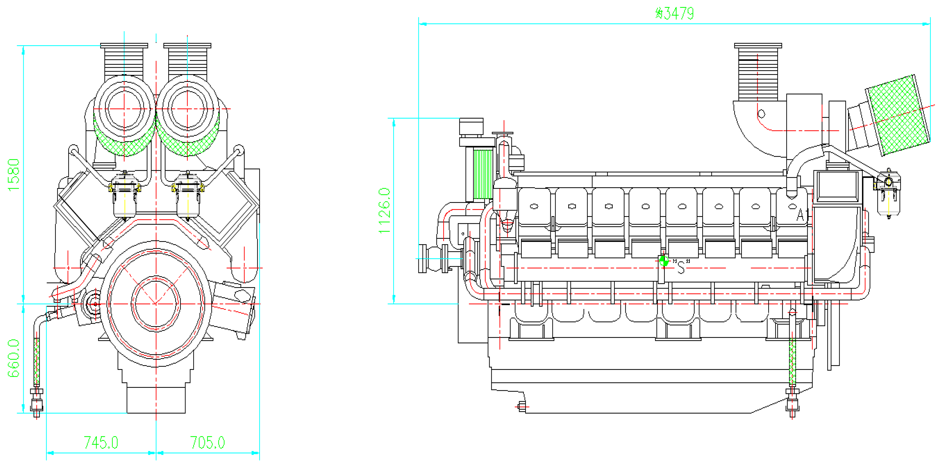
Explosion pressure	16.0 (MPa)

lists the main technical parameters of this type of diesel engine.

Figure 1 the side view and main view of this diesel engine.

4.1. Data Set Introduction.

The object of study is 29 16-cylinder diesel engines of the same type. The data set includes assembly clearance parameter data and quality grade data of the diesel engine. The assembly clearance parameter data of the diesel engine is numerical data, and the quality grade data of the diesel engine is classified data.

The marine diesel engine has a complex structure and many components, so there are many assembly clearance parameters. Chybowski L. and Gawdzixuska K. put forward the latest technology of component importance analysis for complex technical systems [28,29,30]. Choosing important components in complex systems is a key step. This type of diesel engine mainly includes four parts assembly clearance parameters: 2K, 5K, 10K and 11K. Among them, 2K refers to the mating clearance parameters of the crankshaft and the seat hole of the main bearing, 5K refers to the mating clearance parameters of the camshaft and the seat hole, 10K refers to the meshing clearance parameters of the gears, and 11K refers to the mating clearance parameters of the gear hole and the bearing.

Table 2. Assembling clearance parameters adopted.

Parameter Types	Related Components	Number of Parameters
2K	Spindle hole crankshaft and bearing seat	5
5K	Camshaft and its seat	7
10K	Gears	10
11K	Gears and bearings	6

lists the components involved in four types of assembly clearance parameters and the number of parameters.

A total of 28 assembly clearance parameters of the diesel engine were selected, that is, the experimental data set is 28-dimensional. The quality grade data comes from the test run of the diesel engine by the manufacturer before the diesel engine is delivered, including tests on flammability, diesel viscosity, and reliability. Through various test runs, the manufacturer determines the quality grade of the diesel engine. The quality grades are divided into three grades, Qualified, First grade, and High grade.

Table 3. Assembly clearance data and quality grade of the diesel engine.

Diesel Engine ID	2K1	2K2	……	11K6	Machine Quality Grade
1	0.193	0.176	……	0.11	Qualified
2	0.183	0.183	……	0.16	Qualified
3	0.183	0.179	……	0.11	First grade
4	0.174	0.164	……	0.18	High grade
5	0.161	0.167	……	0.15	Qualified
6	0.176	0.175	……	0.15	First grade
⋮	⋮	⋮	⋮	⋮	⋮
29	0.176	0.159	……	0.13	High grade

shows the part of data of the 28 assembly clearance parameters and the corresponding quality grades of the diesel engine.

4.2. Data Pre-Treatment

After the correlation analysis of the dataset, it is obvious that there is a strong correlation between the assembly clearance parameters of the same part of the diesel engine, and this strong correlation will affect the effectiveness and efficiency of the model. Therefore, according to the correlation analysis of the assembly clearance parameters of the diesel engine, the principal component analysis method is used to reduce the dimension of the dataset. Taking all diesel engine assembly clearance parameters as the input, principal component analysis is carried out, and the cumulative variance contribution rate of each principal component is obtained.

As listed in

Table 4. Results of the principal component analysis.

Component	Attribute			Principal Component Contribution Rate
	Total	Ratio of Variance (%)	Cumulative (%)	Total	Ratio of Variance (%)	Cumulative (%)
1	10.934	19.524	19.524	10.934	19.524	19.524
2	6.889	12.302	31.826	6.889	12.302	31.826
3	4.978	8.890	40.717	4.978	8.890	40.717
4	4.112	7.344	48.060	4.112	7.344	48.060
5	3.788	6.765	54.825	3.788	6.765	54.825
6	3.144	5.615	60.439	3.144	5.615	60.439
7	2.672	4.771	65.211	2.672	4.771	65.211
8	2.328	4.157	69.368	2.328	4.157	69.368
9	2.191	3.912	73.280	2.191	3.912	73.280
10	1.901	3.395	76.675	1.901	3.395	76.675
11	1.760	3.142	79.817	1.760	3.142	79.817
12	1.495	2.669	82.486	1.495	2.669	82.486
13	1.447	2.583	85.069	1.447	2.583	85.096
14	1.200	2.143	87.213	1.200	2.143	87.213
15	1.016	1.814	89.027	1.016	1.814	89.027
16	0.923	1.648	90.675
17	0.816	1.457	92.131
18	0.718	1.283	93.414
19	0.664	1.186	94.600
20	0.606	1.082	95.682
21	0.467	0.833	96.516
22	0.438	0.783	97.299
23	0.432	0.772	98.071
24	0.397	0.709	98.780
25	0.252	0.450	99.229
26	0.184	0.328	99.557
27	0.164	0.292	99.850
28	0.084	0.150	100.00

, the cumulative variance contribution rate of the first 15 principal components is up to 89%; that is, these 15 principal components can cover most of the information of the assembly clearance parameters. A new dataset made up of these 15 principal components is presented in

Table 5. A new dataset made up of these 15 principal components.

ID	PC1	PC2	PC3	……	PC15
1	0.908	−0.379	−0.489	……	1.228
2	−0.560	1.453	−0.921	……	−0.206
……	……	……	……	……	……
13	0.339	−0.882	−0.015	……	0.892
14	1.509	0.454	0.669	……	−0.116
15	−0.297	−0.925	0.043	……	1.370
……	……	……	……	……	……
20	−0.295	−0.285	0.915	……	0.243
……	……	……	……	……	……
29	−1.782	0.146	−1.386	……	−0.116

.

The new dataset simplifies the original dataset and retains most of the information contained in the original dataset. Consequently, we can avoid a series of problems that the high-dimensional datasets creates in data mining. Simultaneously, the simplification of the original dataset can improve the efficiency of the model.

Finally, we need to integrate the assembly clearance parameters and whole-quality grades after dimension reduction, and obtain the final dataset that is directly applied to the subsequent computation (see

Table 6. The final dataset.

ID	PC1	PC2	……	PC15	Level
1	0.908	−0.379	……	1.228	qualified
2	−0.560	1.453	……	0.206	qualified
……	……	……	……	……	……
13	0.339	−0.882	……	0.892	First grade
14	1.509	0.454	……	0.116	First grade
……	……	……	……	……	……
20	−0.295	−0.285	……	0.243	First grade
……	……	……	……	……	……
29	−1.782	0.146	……	0.116	High grade

).

4.3. Demonstration of the Process of the Model

Considering the specific object and dataset, the whole quality grades of diesel engine are known in this case, so that the result of partitioning the decisive attribute set to the universe is known in this instance. Therefore, we can simplify the model. We first remove the selected attributes in the decisive attribute set, and relative variables and constraints in the dividing universe. Then, we transfer the variable $q_{i{k}^{\prime }}^{\prime }$ into a parameter matrix, which is known to be a parameter that describes the result of universe partitioning by the decisive attribute set.

The model will be implemented in the MIP solver AMPL/CPLEX (version 12.6.0.1). In the operation of the model, the following parameters need to be set in advance:

1)

Minimum support number of the lower approximation set N = 3,

2)

Variable precision $\beta =0.9$,

3)

A large number M = 999,

4)

The initial condition of the conditional attribute set partitioning universe $q_{11}=1$,

5)

List of the threshold of the similarity of the conditional attribute set ${\alpha }_c=[0.0495,0.0369,\dots ,0.099]$, where c = 15 is the number of assembly clearance parameters in the instance,

6)

The initial number of the approximate equivalence class of the partition of the conditional attribute set to the universe is 10.

The model input consists of the principal component data of the assembly clearance parameters obtained by dimensionality reduction processing, quality grades of the diesel engine, and preset parameters described above. The output of the model includes the selection results of the principal components of the input, division results of the universe according to the conditional attribute set, calculation results of the lower approximation set, and calculation results of the number of elements in the determined region.

Fifteen principal component attributes are included in the conditional attribute set, which is composed of the assembly clearance parameters of a diesel engine. The model can filter the attributes from the attribute set to eliminate the attributes that have little impact on the accuracy of the decision system, and its filtering result are expressed by the variable $\mathrm{s}{l}_c$. The result is:

$$\mathrm{s}{l}_c=\{\begin{array}{c}1\\ 1\\ 1\\ 1\\ 1\\ 1\\ 1\\ 1\\ 1\\ 1\\ 1\\ 1\\ 1\\ 1\\ 1\end{array}\hspace{1em}\begin{array}{c}c=1\\ c=2\\ c=3\\ c=4\\ c=5\\ c=6\\ c=7\\ c=8\\ c=9\\ c=10\\ c=11\\ c=12\\ c=13\\ c=14\\ c=15\end{array}$$

If the $sl$ value of attribute c is 1, this attribute will be selected; otherwise, this attribute will be eliminated. Therefore, the result shows that all 15 principal component attributes will be selected.

The conditional attribute set partitioning the universe is an important step in the calculation process of the model. Meanwhile, it is also the prerequisite for the subsequent calculation; $k=10$ represents the 10 approximate equivalence classes. If a diesel engine belongs to an approximate equivalence class, the value of the element in the matrix is 1; otherwise, it is 0. The result is:

$$Q_k=\{\begin{array}{c}\begin{array}{c}4\\ 4\\ 4\end{array}\\ 3\\ 4\\ 3\\ 0\\ 3\\ 1\\ 3\end{array}\hspace{1em}\begin{array}{c}\begin{array}{c}k=1\\ k=2\\ k=3\end{array}\\ k=4\\ k=5\\ k=6\\ k=7\\ k=8\\ k=9\\ k=10\end{array}$$

This result indicates the number of diesel engines in each approximate equivalence class obtained by the partitioning of conditional attribute set to the universe. Among the 10 approximate equivalence classes, one has not been allocated any element; this approximate equivalence class will be deleted. One has been allocated only one element, and its number is less than the minimum support number; therefore, it will also be deleted. Only eight approximate equivalence classes can be regarded as the lower approximation set.

$$E=\left[\begin{array}{c}\begin{array}{c}0\\ 0\\ 0\end{array}\\ 0\\ 4\\ 0\\ 0\\ 0\\ 0\\ 3\end{array}\hspace{1em}\begin{array}{c}\begin{array}{c}0\\ 4\\ 4\end{array}\\ 3\\ 0\\ 0\\ 0\\ 3\\ 0\\ 0\end{array}\hspace{1em}\begin{array}{c}\begin{array}{c}4\\ 0\\ 0\end{array}\\ 0\\ 0\\ 3\\ 0\\ 0\\ 1\\ 0\end{array}\right]$$

The E matrix is the most important part of the model output. The E matrix represents the number of elements that not only belong to approximate equivalence class c, but also belong to one quality grade. E matrix is an important basis for solving the lower approximation set. In the E matrix for this case, the 10 lines indicates that the number of approximate equivalence classes determined by conditional attribute set partitioning of the universe is 10. Similarly, the number of approximate equivalence classes determined by decisive attribute set partitioning of the universe is 3.

$$Y_k=\{\begin{array}{c}\begin{array}{c}4\\ 4\\ 4\end{array}\\ 3\\ 4\\ 3\\ 0\\ 3\\ 0\\ 3\end{array}\hspace{1em}\begin{array}{c}\begin{array}{c}k=1\\ k=2\\ k=3\end{array}\\ k=4\\ k=5\\ k=6\\ k=7\\ k=8\\ k=9\\ k=10\end{array}$$

$Y_k$ is the number of elements in each lower approximation set. It can be concluded that eight approximate equivalence classes meet the condition of being members of the lower approximate set by analyzing the minimum support number and variable precision. Hence, the number of elements in the determined area is:

$${\displaystyle \sum }_{k=1}^{15}{Y}_k=28$$

The area of the model is:

$$\mathsf{\lambda }=\frac{{{\displaystyle \sum }}_{k=1}^{15}{Y}_k}{\left|I\right|}=0.97$$

On the basis of the inferences of the rough set and the function dependence, $0<\mathsf{\lambda }<1$. Thus, there is partial dependence between the conditional attribute set and the decisive attribute set of the decision system:

$$\{\mathrm{assembly}\mathrm{clearance}\mathrm{parameter}\}{\to }_{0.97}\{\mathrm{quality}\mathrm{grade}\}$$

4.4. Performance Comparison of Models

To validate the effectiveness and advantages of the model, experiments are performed to compare the accuracy of the models. The model that our model is compared to is the Φ-rough set.

As listed in

Table 7. Comparison of the accuracy of the two models.

Model	$\mathsf{\lambda }$
Φ-Rough set	0.68
MILP-FRST	0.97

, obviously, the accuracy of model MILP-FRST is higher than that of the model Φ-Rough set. The accuracy is close to one, which shows that our proposed model can establish an accurate decision-making rule between the diesel engine assembly clearance parameters and whole machine quality grades, and excavate a higher correlation between them.

MILP-FRST is an extension of the rough set. An obvious characteristic of a linear model is its ability to find the optimum solution. This characteristic enables the model to find the best way to classify attributes, even if the dataset can also obtain ideal results merely through simple data preprocessing, and it considerably increases the ability to resist noisy data.

4.5. Extension of the Model

As mentioned above, the minimum support number of the lower approximation set N and variable precision $\beta$ are set in advance. The classification quality reflects the degree of dependence of decisive attribute D on the conditional attribute C and the uncertainty of decision system. The classification quality is inversely proportional to the uncertainty. In the model, the classification quality largely depends on the value of $\beta$ [31]. Practically, the user does not always know how to set the value of $\beta$ to obtain the maximum accuracy model. The minimum support number of the lower approximation set N also influences the accuracy of the model. Similarly, the user always sets the value of N in accordance with their experience. 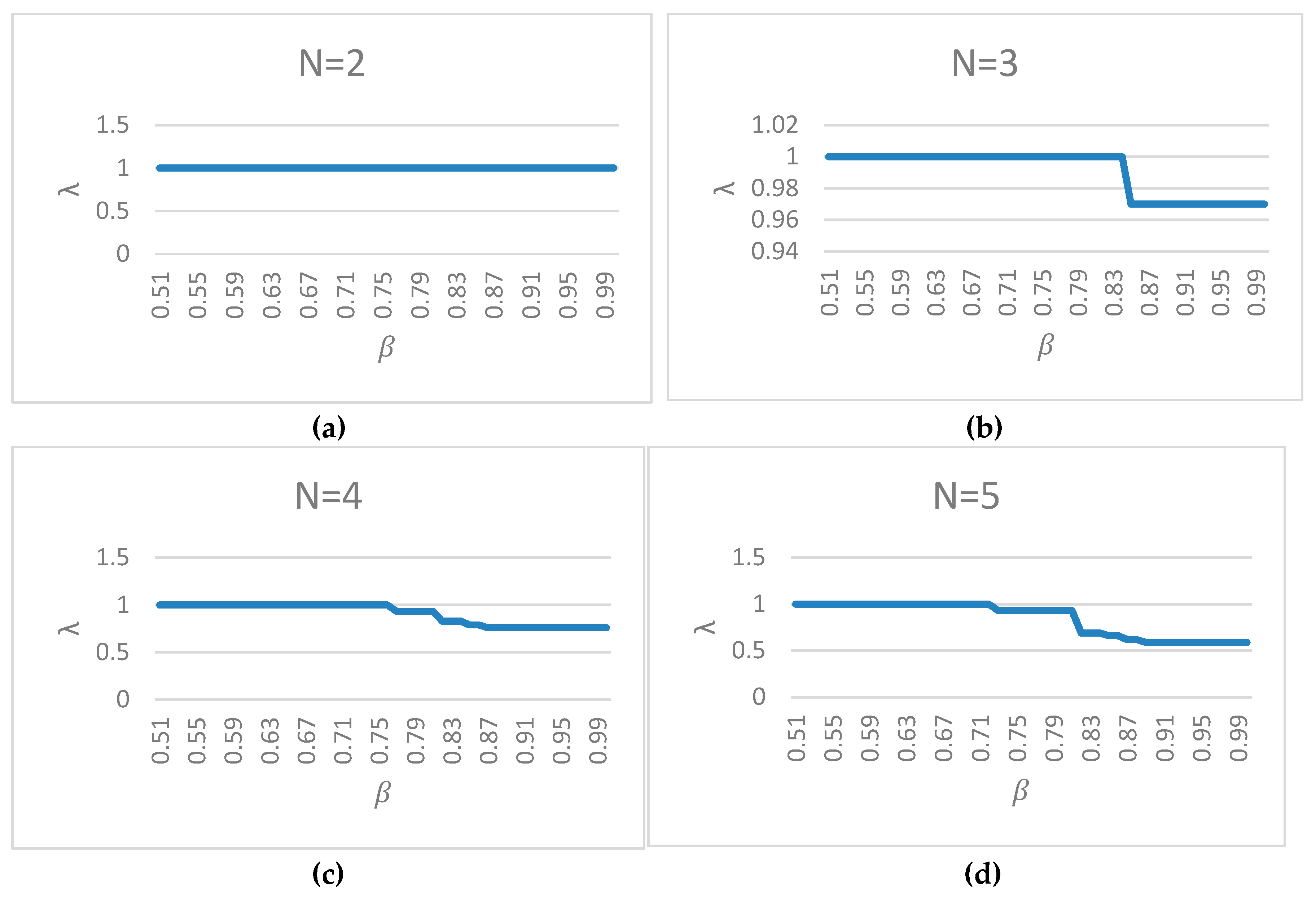To determine the best value of $\beta$ and N, we propose an algorithm. We set up a loop traverses all the values between 0.5–1, adding 0.01 each time. The results of the different N values are shown in Figure 2.

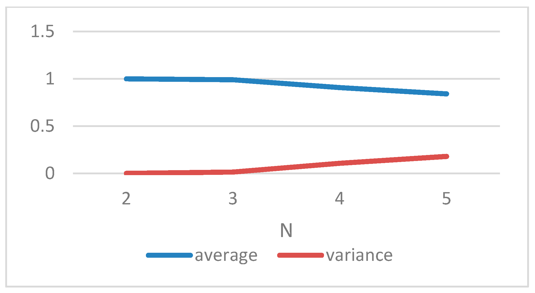
As shown in Figure 3, it is obvious that with the increase in N, the average of λ decreases and the variance of λ increases.

Although the model’s accuracy increases when $\beta$ decreases, for this model, the smaller $\beta$ does not make the model better. $\beta$ represents the tolerance degree of the rough set to noisy and incorrect information in the dataset, while a smaller $\beta$ tolerates more noisy data, but this violates our purpose in building MILP-FRST. Therefore, how to balance $\beta$ against λ requires further research. As for the minimum support number N, our results indicate that the smaller the N, the better the λ. This rule is useful in practical applications, but when using this rule, the characteristics of the object should be considered to determine the appropriate N.

5. Conclusions

The purpose of this paper is to establish an accurate decision-making method between the quality level of the diesel engine and the parameters of assembly clearance. Therefore, a novel mixed-integer linear programming model for the rough set-based classification with flexible attribute selection, called MILP-FRST, is presented. First, the correlation between the conditional attribute set and decisive attribute set according to the inference of the rough set and function dependence is calculated. Second, by integrating the data mining model with the mixed integer linear programming theory, the optimization method is studied with regard to the sensitivity of the rough set to noisy data. Integrating the MILP model with the rough set model, the related theories and concepts of the rough set are implemented in the model, and the extension of the rough set research is completed. Finally, a case study on test data from a diesel engine is carried out. Experiments show that the decision-making method proposed in this paper can realize the quantitative discussion of the relationship between assembly clearance and the quality level of the whole machine. Also, the effectiveness of and the advantages of the MILP-FRST are verified. Furthermore, the extension of the MILP-FRST indicates that the usage of the minimum support number N and related topics are worthy of more in-depth study.