A Projection of Extreme Precipitation Based on a Selection of CMIP5 GCMs over North Korea


1
Ministry of Environment, Han River Flood Control Office, Seoul 06501, Korea
2
K-Water Convergence Institute, K-Water, Daejeon 34045, Korea
3
Department of Statistics, University of Seoul, Seoul 02504, Korea
4
Division for Integrated Water Management, Korea Environment Institute, Sejong 30147, Korea
*
Author to whom correspondence should be addressed.
Sustainability 2019, 11(7), 1976; https://0-doi-org.brum.beds.ac.uk/10.3390/su11071976
Submission received: 15 March 2019
/
Revised: 28 March 2019
/
Accepted: 2 April 2019
/
Published: 3 April 2019
(This article belongs to the Special Issue Uncertainty of Climate Change Impacts on Hydrology, Water Quality and Ecology)
Abstract
:The numerous choices between climate change scenarios makes decision-making difficult for the assessment of climate change impacts. Previous studies have used climate models to compare performance in terms of simulating observed climates or preserving model variability among scenarios. In this study, the Katsavounidis-Kuo-Zhang algorithm was applied to select representative climate change scenarios (RCCS) that preserve the variability among all climate change scenarios (CCS). The performance of multi-model ensemble of RCCS was evaluated for reference and future climates. It was found that RCCS was well suited for observations and multi model ensemble of all CCS. Using the RCCS under RCP (Representative Concentration Pathway) 8.5, the future extreme precipitation was projected. As a result, the magnitude and frequency of extreme precipitation increased towards the farther future. Especially, extreme precipitation (daily maximum precipitation of 20-year return-period) during 2070-2099, was projected to occur once every 8.3-year. The RCCS employed in this study is able to successfully represent the performance of all CCS, therefore, this approach can give opportunities managing water resources efficiently for assessment of climate change impacts.
1. Introduction
Due to climate change, heavy rainfall events associated with meso-scale convective processes frequently occur during the East Asian summer monsoon [1,2,3]. The average temperature over North Korea has risen by 1.9 ℃ as observed over the past 100 years, which is the second highest increase worldwide. Generally, both climate change scenarios and long-term observations have been employed in assessing the impacts from climate change. In order to investigate trends from the observed hydrological variables in South and North Korea, Kim et al. [4] analyzed daily precipitation data of North Korea from 1983 to 2007 and of South Korea over a period of 35 years from 1973 to 2007. This study identified a clear decrease in summer precipitation across North Korea. By contrast, the opposite occurred in South Korea. Sung et al. [5] assessed meteorological hazards based on trends in precipitation for the Korean peninsula. The results suggested that the Annual Daily Maximum Precipitation (ADMP) in North Korea increased at four sites and decreased at three sites. North Korea is known to be under threat from climate change, and was ranked 2nd in the world in 2009 on the Global Climate Risk Index [6,7].
Climate change scenarios have been extensively used to assess impacts from extreme events [8,9,10,11,12], but the Global Circulation Models (GCMs) include significant uncertainties. For impact assessment concerning extremities of climate, it is necessary to quantify uncertainties caused by different dynamic systems, grid sizes simulated and parametrization physics. To quantify the uncertainty in climate change scenarios, many studies recommend the use of multi-models [13,14,15,16,17] or the selection of representative scenarios [18,19]. Several studies have suggested that scenarios should be weighted appropriately for the ensemble results [20,21]. To weight scenarios, Bayesian updating methods have been widely used to weight different members or models [22,23,24]. The previous studies demonstrated that the performance of predictability of the multi-model forecast assigning appropriate weights on individual models using Bayesian updating scheme can be enhanced. Nonetheless, the Intergovernmental Panel on Climate Change (IPCC) adopts the ‘one-model-one-vote’ for the CMIP3 (Coupled Model Inter-comparison Project Phase 3) and CMIP5 projections, assuming that the likelihood of each scenario is the same [25]. The use of as many models as possible has been recommended. However, the consideration of multiple scenarios is costly and time-consuming work so it can be difficult to make decisions. Therefore, studies have been conducted to select a few specific (representative) scenarios.
Until now, scenarios have been mainly selected based on the performance in reproducing the historical (observed) climate, but the reproducibility of past climate cannot guarantee the future climate projection. Therefore, in recent research, a methodology has been developed that can reflect inter-model variability to select a subset of the GCM [26,27]. In order to select suitable representative scenarios, cluster analysis such as k-means has primarily been used [28,29]. After Katsavounidis et al. [30] proposed the Katsavounidis-Kuo-Zhang (KKZ) algorithm, Cannon et al. [31] and Chen et al. [32] demonstrated the superiority of the KKZ algorithm over approaches based on clustering in terms of preserving the entire inter-model variability. Seo et al. [18] then employed the KKZ algorithm to select a subset of GCMs based on indices associated with extreme changes in climate.
Climate change scenarios produced on a national level contain high-quality data with different dynamics that may be a good choice for producing all possible outcomes. However, for countries that are trying to assess impacts using limited resources, it may be preferable to assess climate change impacts using selected representative scenarios. In this case, it may be a reasonable alternative to use techniques that can capture as extensive a range of inter-model variability in the future as possible while keeping the number of GCMs used at a minimum. For instance, despite the urgency to assess impacts using climate change scenarios in North Korea, there are few case studies projecting extreme precipitation in North Korea in the future. Hence, the first goal of this study is to select climate change scenarios which can represent inter-model variability using downscaled GCMs at a local scale. The second goal is to evaluate the ensemble mean of the selected scenarios by comparing observation with the ensemble mean of all the scenarios. Along with an evaluation of the performance of the representative scenarios, this study aims to predict the possibility of extreme precipitation in the future of North Korea.
2. Materials and Methods
2.1. Overview
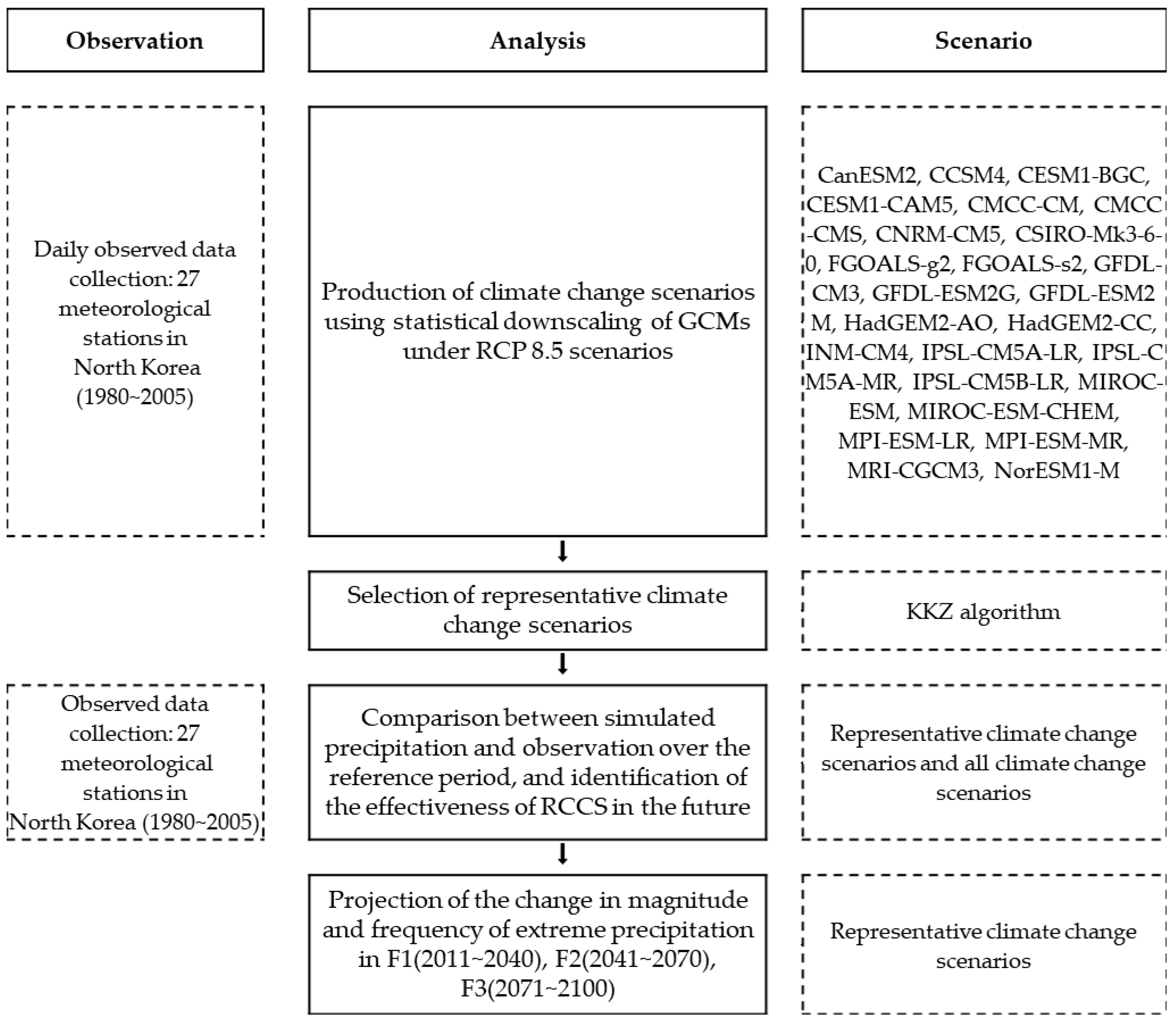
In this study, we used an MME (Multi-Model Ensemble) approach, which combines results from multiple models in order to project changes in and return periods of possible extreme precipitation in North Korea. Figure 1 illustrates the overall process of this study. By employing the daily precipitation series from 25 CMIP5 climate projections that were downscaled using a statistical downscaling scheme, we collected the annual maximum daily precipitation in North Korea. The KKZ algorithm was used to select representative climate change scenarios (RCCS) for extreme precipitation as defined from observations of a 20-year period of precipitation. We projected the frequency and magnitude of extreme precipitation using the Generalized Extreme Value (GEV) distribution both for the reference period (1980~2005) and for the three 30-year future periods (F1: 2011~2040, F2: 2041~2070, and F3: 2071~2100) (Figure 1).
2.2. Climate Change Scenarios
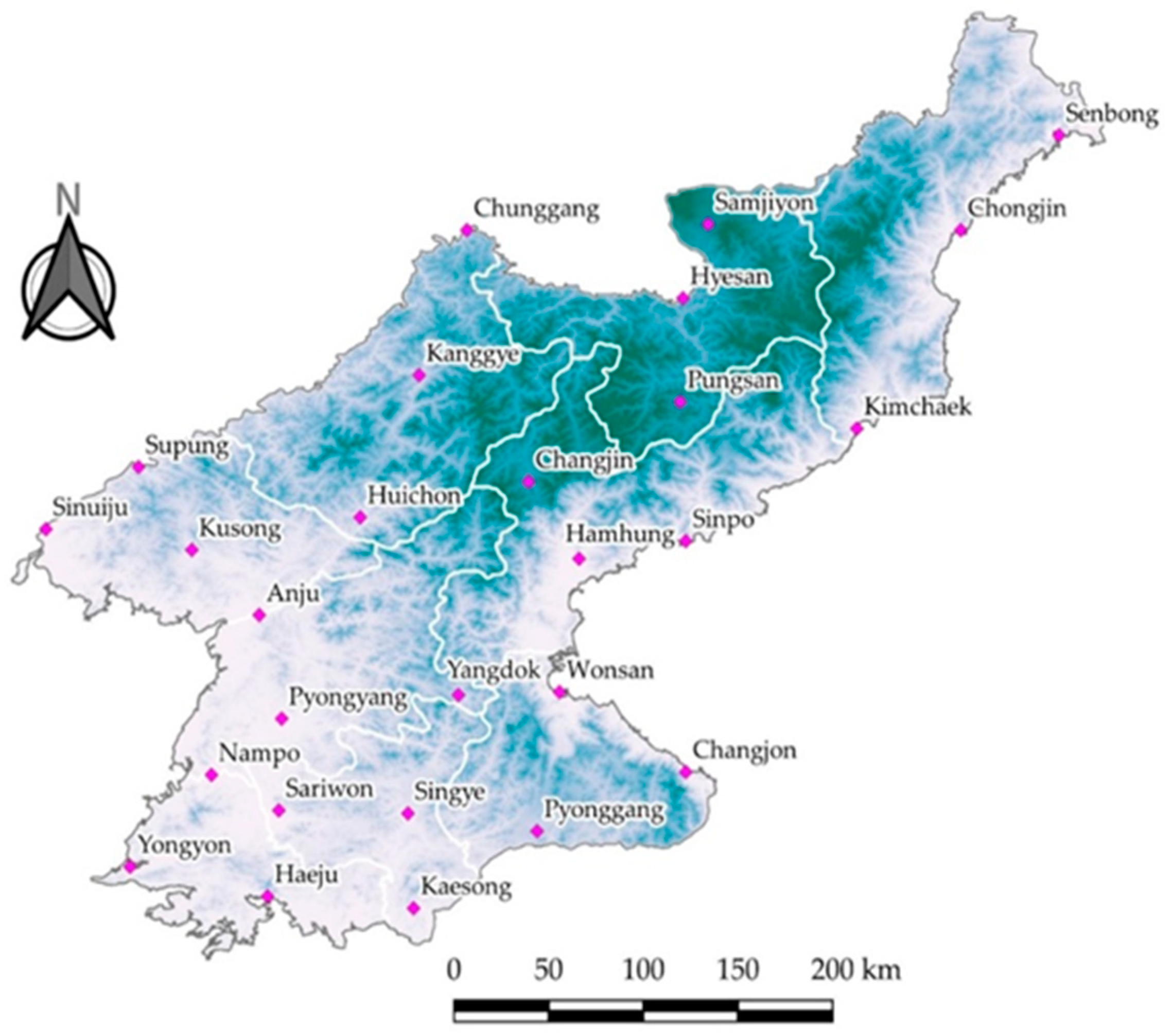
North Korea is the northern region of the Korea Peninsula, divided by the Military Demarcation Line (MDL), which was established in the armistice agreement of July 1953. The area covers 123,138 km2, thereby occupying 55.1% of the total 223,477 km2 of the Korean Peninsula (Figure 2, Kwon et al., 2019). Since North Korea is in contact with Manchu and Siberia to the north, it is relevant as the connection between continent and ocean. More than 80% of the country is mountainous, and North Korea has a continental climate with four seasons. The long winter season brings very cold and clear weather, with numerous snow storms that result from the northern Siberian winds. The summers are extremely hot, humid, and rainy because of the southern monsoon winds that bring moist air from the Pacific Ocean.
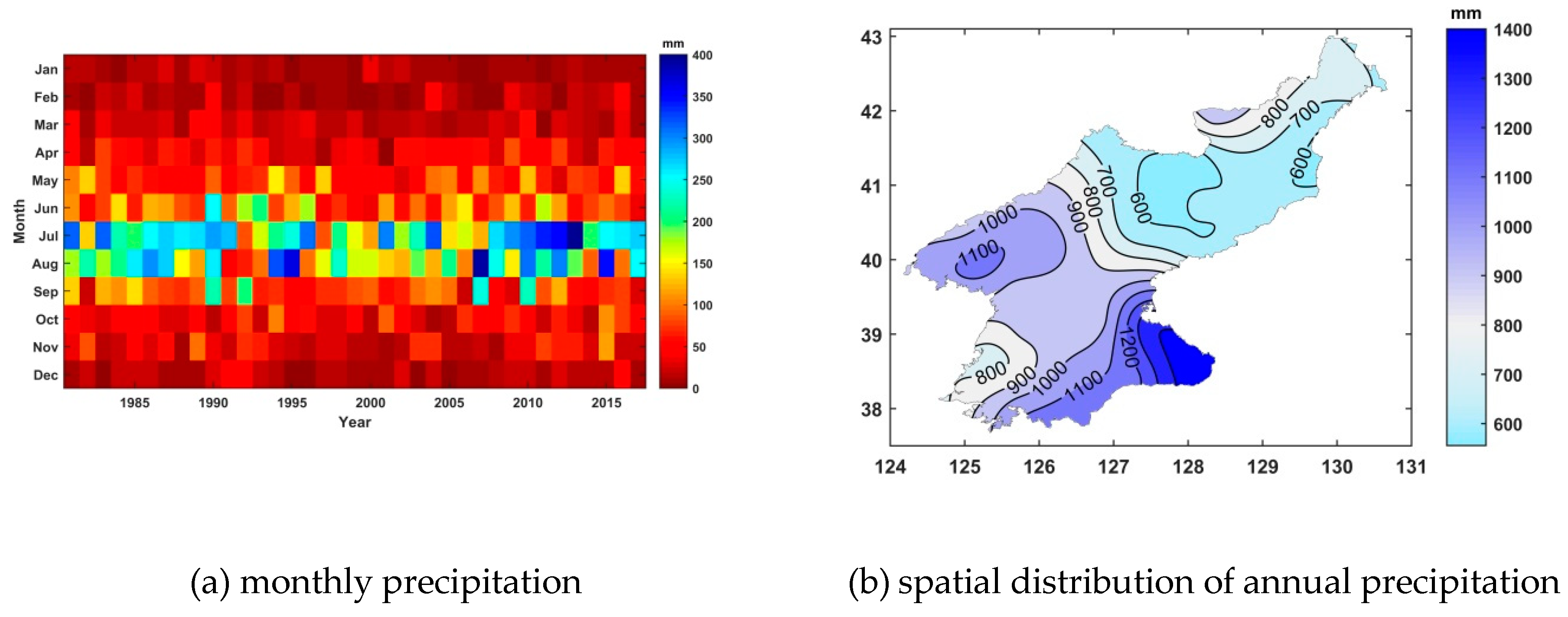
The monthly precipitation from 27 stations over North Korea was analyzed to identify both monthly and seasonal variability (Figure 3). July and August receive the highest annual precipitation at 48.1% of the total annual rainfall (969.3 mm), with relatively low precipitation in winter and spring. The amount of precipitation in July is increasing; in July 2013, rainfall for this month alone reached 811.2 mm (as shown in Figure 3a). The Gaema Plateau in the North receives less precipitation than other regions, with both the area around the Chungcheon River and the region near the MDL suffering from the highest amounts of rainfall in North Korea (as shown in Figure 3b).
This study employed climate change scenarios at local scale of 27 weather stations from which the 25 GCMs for the scenarios were downscaled (Table 1). Using climate projections at the grid points of each GCM, we applied a statistical downscaling method to downscale to the weather stations as in Figure 2. In Coupled Model Inter-comparison Project Phase 5 (CMIP5) we used the RCP (Representative Concentration Pathways) 8.5 scenario which represents the pathway using the highest greenhouse gas emissions.
The APCC (APEC Climate Center) Integrated Modeling (AIMS) produced downscaled climate projection data of South Korea using two BCSD (Bias-Correction Spatial Disaggregation) methods [17]; the SQM (Simple Quantile Method) and Spatial Disaggregation with Quantile Delta Mapping (SDQDM) [33] which can retain long-term temporal trends in climate. This study used the SDQDM method to downscale future projections of daily precipitation and temperature of 25 GCMs from CMIP5 under RCP 8.5 to locations of the 27 weather stations.
2.3. Theory
The KKZ algorithm [30] was applied to select representative climate change scenarios—GCMs in this study—for North Korea. The KKZ algorithm was designed to select models that cover the spread of an ensemble with sufficient characterization of high-density regions in multi-variate space [18,34]. Given the N number of GCMs and the P number of climate variables, the KKZ algorithms were applied as follows:
- For the first GCM, the model that is located closest to the centroid of the ensemble; i.e., the model with the lowest sum of squared errors (SSE) at the centroid across all of the climate variables is determined, as shown by Equation (1):where is the value of the pth climate variable for the ith model, and is the centroid value of the pth climate variable across all the models.For the second GCM, the model that lies farthest from the first model is selected. The p-space Euclidean distance is used to calculate the distance, , between the two models (the ith and jth GCMs):
- For selection of the rest of the GCMs (from the 3rd to the last selection)
- (i)
- the distances from each remaining model to the previously selected models are calculated;
- (ii)
- only the lowest distance among those calculated in step 3(i) for each remaining model is retained;
- (iii)
- the model with the maximum distance among those chosen in step 3(ii) is determined as the next model.
- Step 3 is repeated until all the models have been selected in order. Readers are referred to Seo and Kim [19] for an example of the step-by-step procedure used with a simple bi-variate case.
The GEV distribution has been widely used to describe extremities in hydro-meteorological variables [35,36,37]; because the GEV distribution includes three different limiting distributions of extreme value depending on the shape parameter value. The cumulative distribution function, which estimates the non-exceedance probability, can be estimated by Equation (3) and its solution is estimated using Equation (4) [38]:
where , , and are location, scale, and shape parameters, respectively. Because the GEV is represented by for , it follows that if , the distribution has a thicker right-hand tail. We used the GEV type II distribution. Among the parameters estimation scheme, the method of L-moment is not sensitive to outliers because of the order statistics of the data [39]. In this study, the method of L-moment was applied to estimate the parameters. Klein Tank et al. [40] suggested a return period of 20 years for evaluating the magnitude and frequency of rare events that lie far in the tails of the probability distribution of weather variables. We selected extreme precipitation as a target under a 20-year return period.
3. Scenario Selection and Evaluation
3.1. RCCS Selection
All the GCMs were placed into order by the KKZ algorithm corresponding to both the total annual precipitation and extreme event (1-day maximum precipitation) variables during the reference period (F3, 2071-2010). RCCS were then selected, and ranking from 1st to 5th, GCMs chosen were: FGOALS-s2, GFDL-ESM2G, HadGEM2-CC, CanESM2, and IPSL-CM5A-MR. It is anticipated that uncertainties in precipitation can be explained by the RCCS. The performance of the RCCS is discussed in the following section.
3.2. Evaluation of Performance during the Reference Period
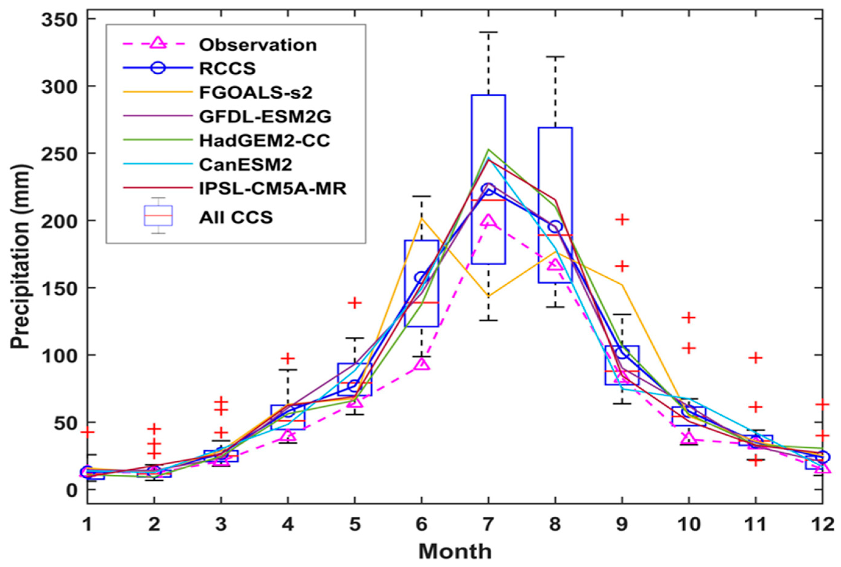
Many studies have quantified the uncertainty among scenarios through use of a MME of climate change scenarios (CCS), and the weight of the MME has been determined by comparing the model simulations with observations over a reference period [41,42]. Five scenarios were selected as the RCCS for extreme precipitation in North Korea, and the ensemble mean of these scenarios is expected to be similar to the ensemble mean of all scenarios. Therefore, in this section, the simulated and observed monthly precipitation for the reference period was compared to assess the performance of the precipitation simulation. Figure 4 shows the monthly precipitation determined from all CCS, the RCCS, each scenario of RCCS, and observation. Results indicated that most of the scenarios reflected the monthly and seasonal variability apparent from observation. The correlation coefficient was compared, of which FGOALS-s2 was the lowest at 0.81. All CCS and RCCS were 0.98, which highly correlated with observation. The rest were all above 0.95.
We evaluated the performance and effectiveness of the RCCS by comparing the difference between all CCS, RCCS, each scenario of RCCS and observation (Figure 5). At Changjon, which is a region with high precipitation (see Figure 2), simulated precipitations in most scenarios were lower than observations. However, simulated precipitation was greater than observation for Pungsan, Sinpo, Anju, Pyongyang, and Singye, all of which have less annual mean precipitation. The absolute deviation between each scenario was calculated and compared with the mean value of total absolute deviation. Results showed that the all CCS maintained the best performance, which was the smallest at 48.5mm. The RCCS was the next best at 50.1mm, which is not significantly different from the results of all CCS.
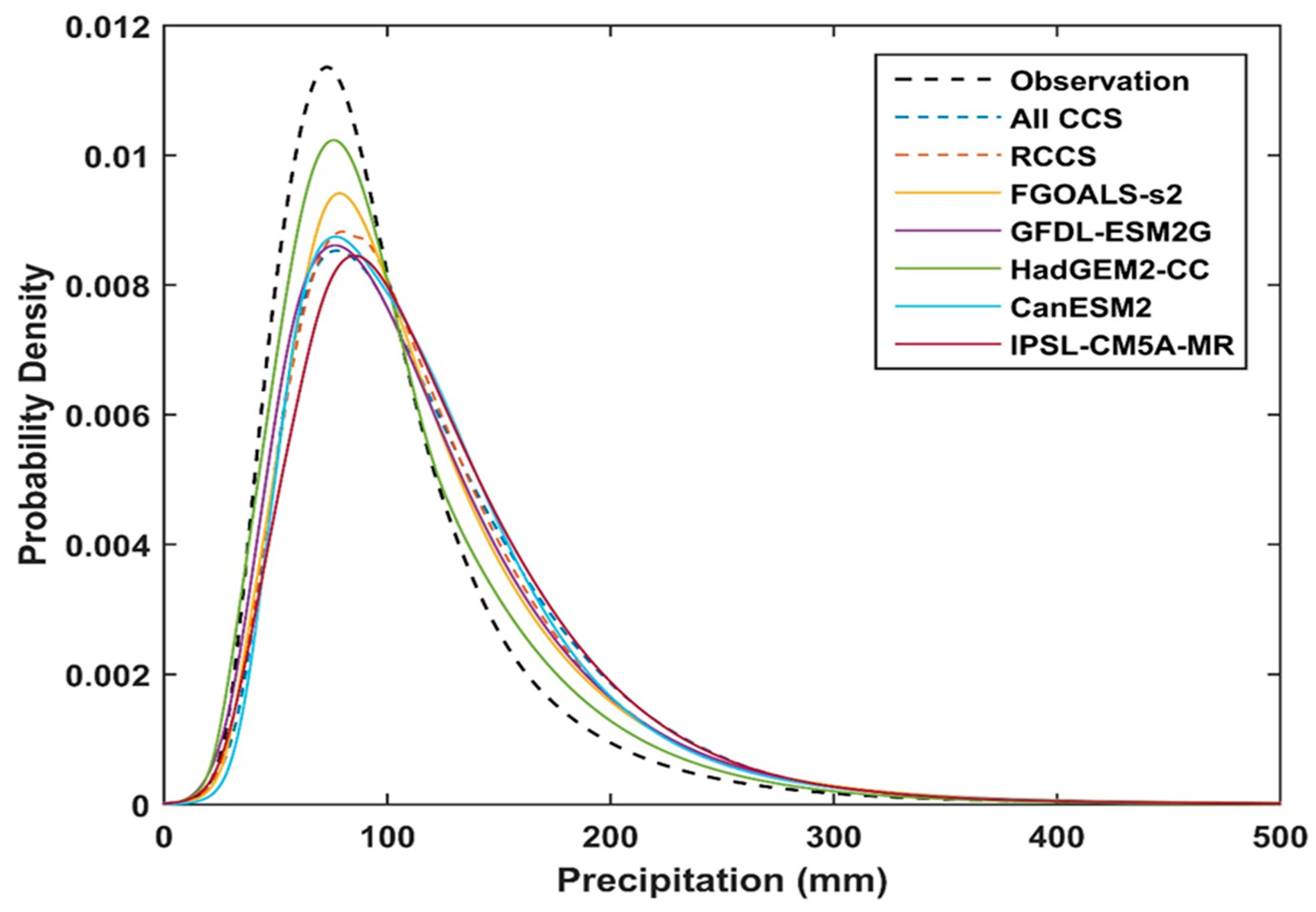
To confirm the performance of the simulations for extreme precipitation caused by climate change, we compared the 20-year frequency precipitation of all CCS, RCCS, each scenario of RCCS, and observation for the reference period. Table 2 shows the estimated values of GEV distribution parameters—location, scale and shape parameters—for each scenario. Figure 6 shows the probability density function (PDF) for each scenario. The location and scale parameters were largely estimated from comparisons of the scenarios with the observations. The extreme precipitation in the scenarios was greater than the observations, and the variation across the scenarios was significant. The median of the PDFs of the scenarios moved to the right when compared to observation, and the horizontal widths of the PDFs were wider. Thus, it is projected that magnitude and frequency of extreme precipitation will increase in comparison to observation.
4. Discussion
4.1. An Evaluation of the Performance for Future Analysis
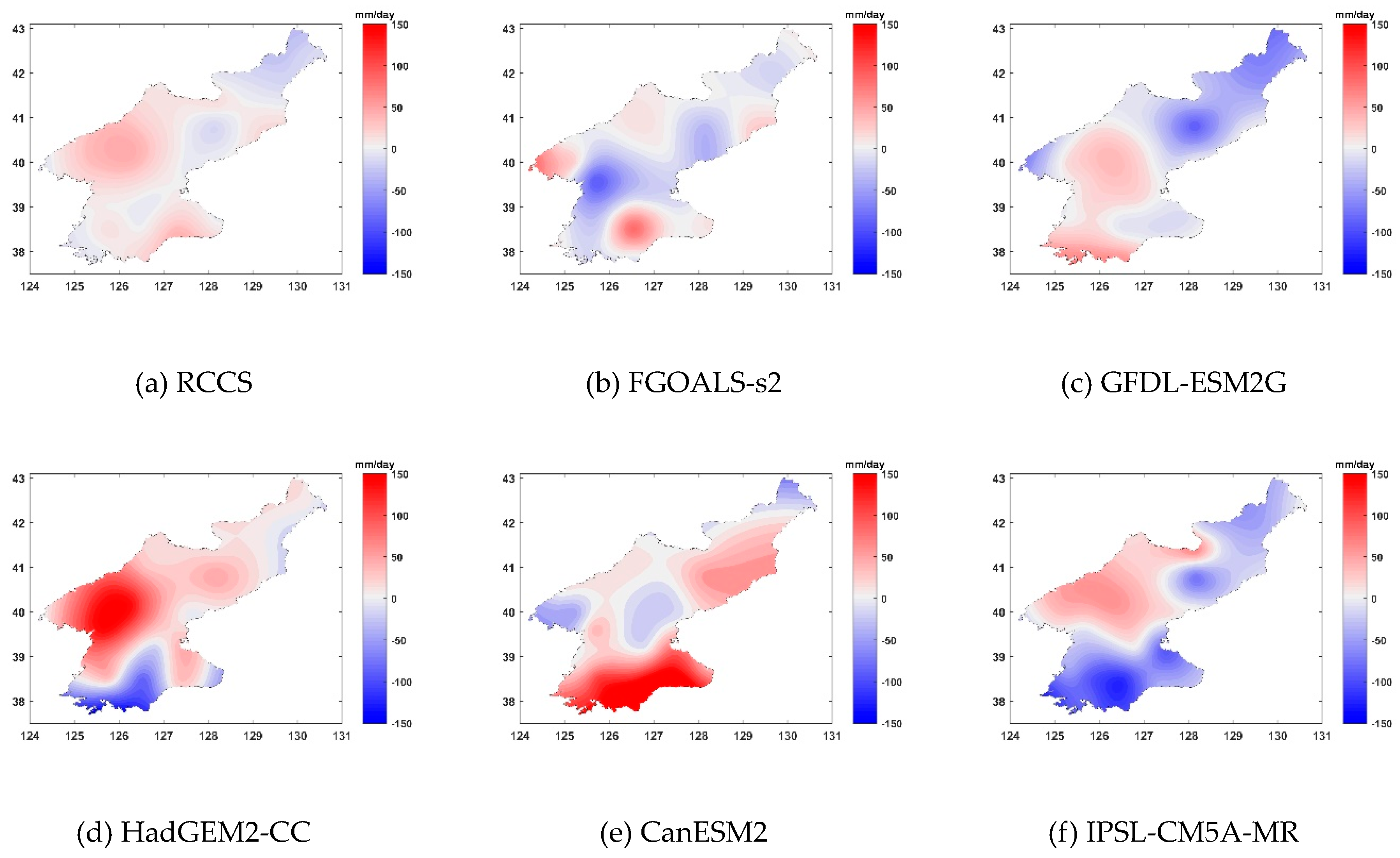
We compared the performance of the scenarios over the reference period in Section 3, and confirmed that the performance of the RCCS was adequate. This section compares the projection performance of the RCCS with the extreme precipitation of the late 21st century. First, we compared the magnitude of extreme precipitation for each scenario in the F3 (2071~2100) period. Figure 7 shows the difference between the RCCS, each five scenarios of RCCS and all CCSs in F3. The darker red and blue colors in the figure point to large differences from all CCS. As a result of comparing the spatial distribution of the differences, RCCS was smaller than all CCS (as shown in Figure 7a). The spatial averaged absolute deviation (range) in each scenario was calculated and quantitatively analyzed. As a result, the mean absolute deviations of RCCS, FGOALS-s2, GFDL-ESM2G, HadGEM2-CC, CanESM2, and IPSL-CM5A-MR were calculated at 12.8, 22.7, 23.5, 47.7, 55.5, and 43.9 mm, respectively. The RCCS was the smallest, and it was confirmed that there were under- and over-estimations in five scenarios corresponding to the RCCS around the MDL (as shown in Figure 7b–f). While CanESM2 (Figure 7e) produced the most over-estimated value, in contrast, IPSL-CM5A-MR (Figure 7f) produced the most under-estimated value.
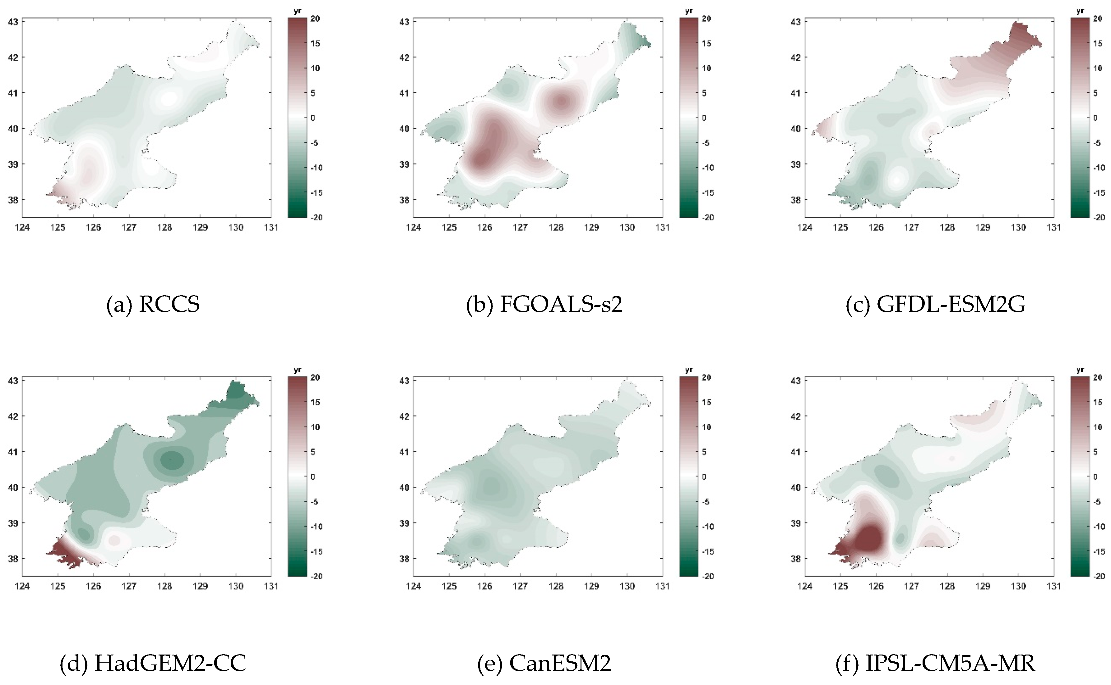
Next, we investigated the changes in the return period of extreme precipitation in F3 as compared to the reference period (20 years). Figure 8 shows the difference between the RCCS, the five scenarios included in the RCCS, and all CCS, where the darker green and brown colors of the figure mean significant differences from all CCS.
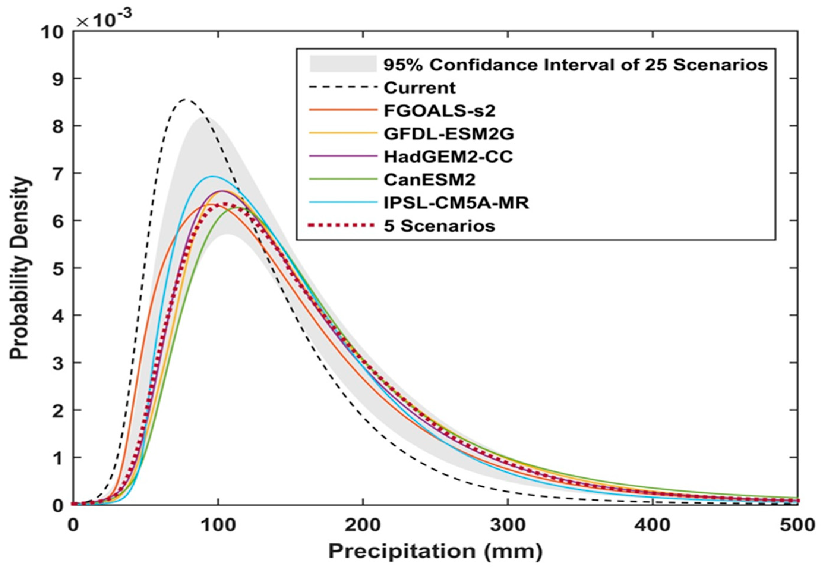
As shown in Figure 8a, use of the RCCS led to the smallest difference from all CCS. As a result, the mean absolute deviations of RCCS, FGOALS-s2, GFDL-ESM2G, HadGEM2-CC, CanESM2, and IPSL-CM5A-MR were calculated at 1.9, 3.9, 4.0, 6.4, 3.9 and 5.7 years, respectively. In terms of differences in spatial distribution, there was significant variability when comparing all CCS to HadGEM2-CC and IPSL-CM5A-MR. This is because the spatial variability (among sites) increased due to the wide horizontal band of the PDFs obtained by HadGEM2-CC and IPSL-CM5A-MR (Figure 9).
4.2. Future Projections Based on RCCS
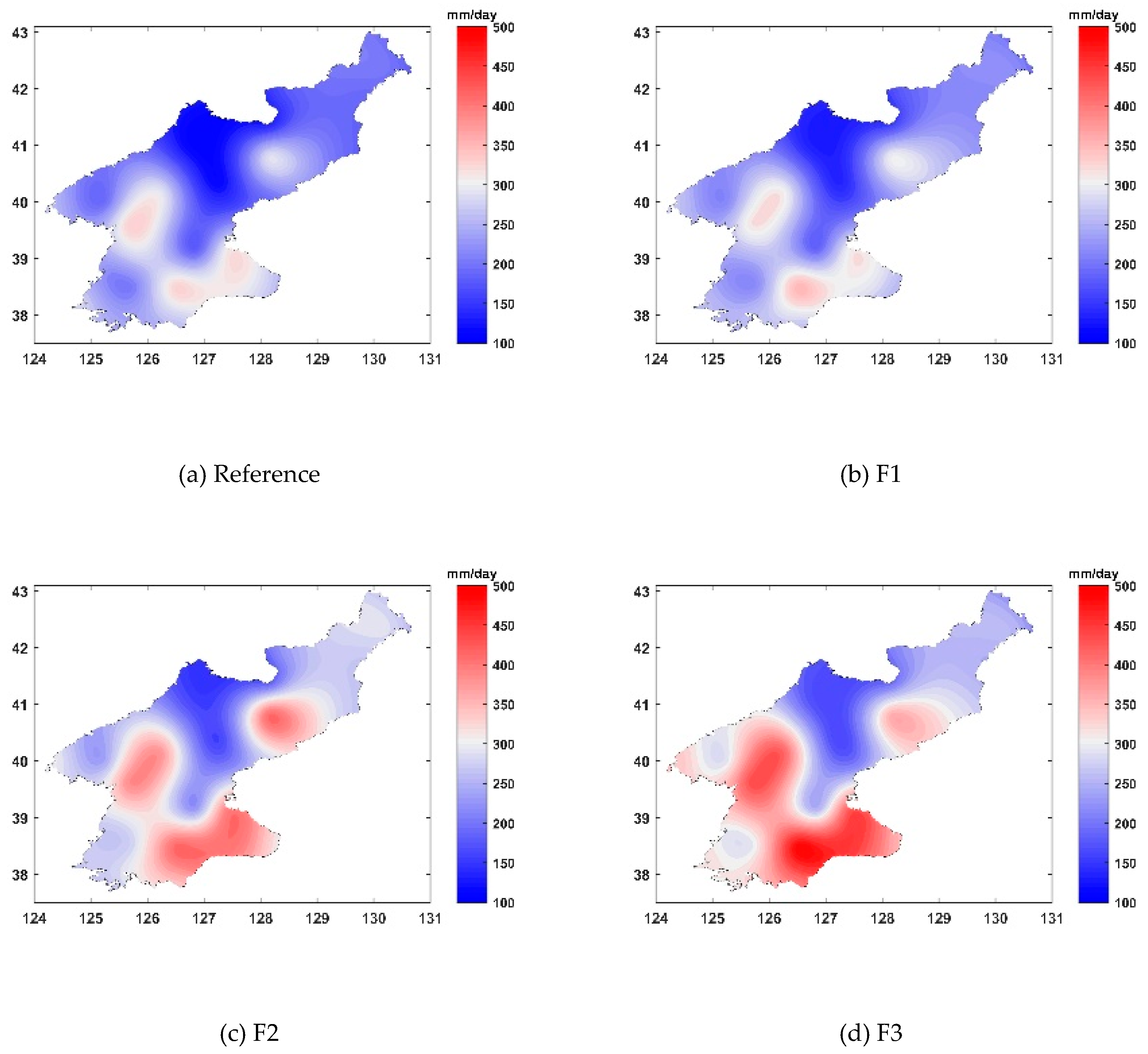
The performance of the RCCS and all CCS during the reference and future (F3) periods was similarly assessed. We also projected the magnitude and frequency of extreme precipitation throughout the 21st century, F1 (2011~2040), F2 (2041~2070) and F3 (2071~2100) using RCCS as presented in Figure 10. The average for the 20-year precipitation frequency of the 25 GCMs changed gradually from the reference period and through the F1, F2 and F3 periods. The 20-year precipitation frequency during the reference period was 227.0 mm/day (Figure 10a); this was expected to increase by 5.2% (F1), 27.9% (F2), and 39.9% (F3) in comparison with the present (Figure 10b–d). As a result of comparing the spatial distribution, larger precipitation was projected near the upper- and mid- Chuncheon River and around the MDL adjacent to South Korea. The region including the Anju and Huichon stations at the mid- and upstream Cheongcheon River is an area undergoing high precipitation because of a topographic effect. In regions near the MDL, the rate of increase in precipitation is very high compared to other regions, and Pyongyang, Singye and Kaesong were expected to increase by more than 50% compared to the present.
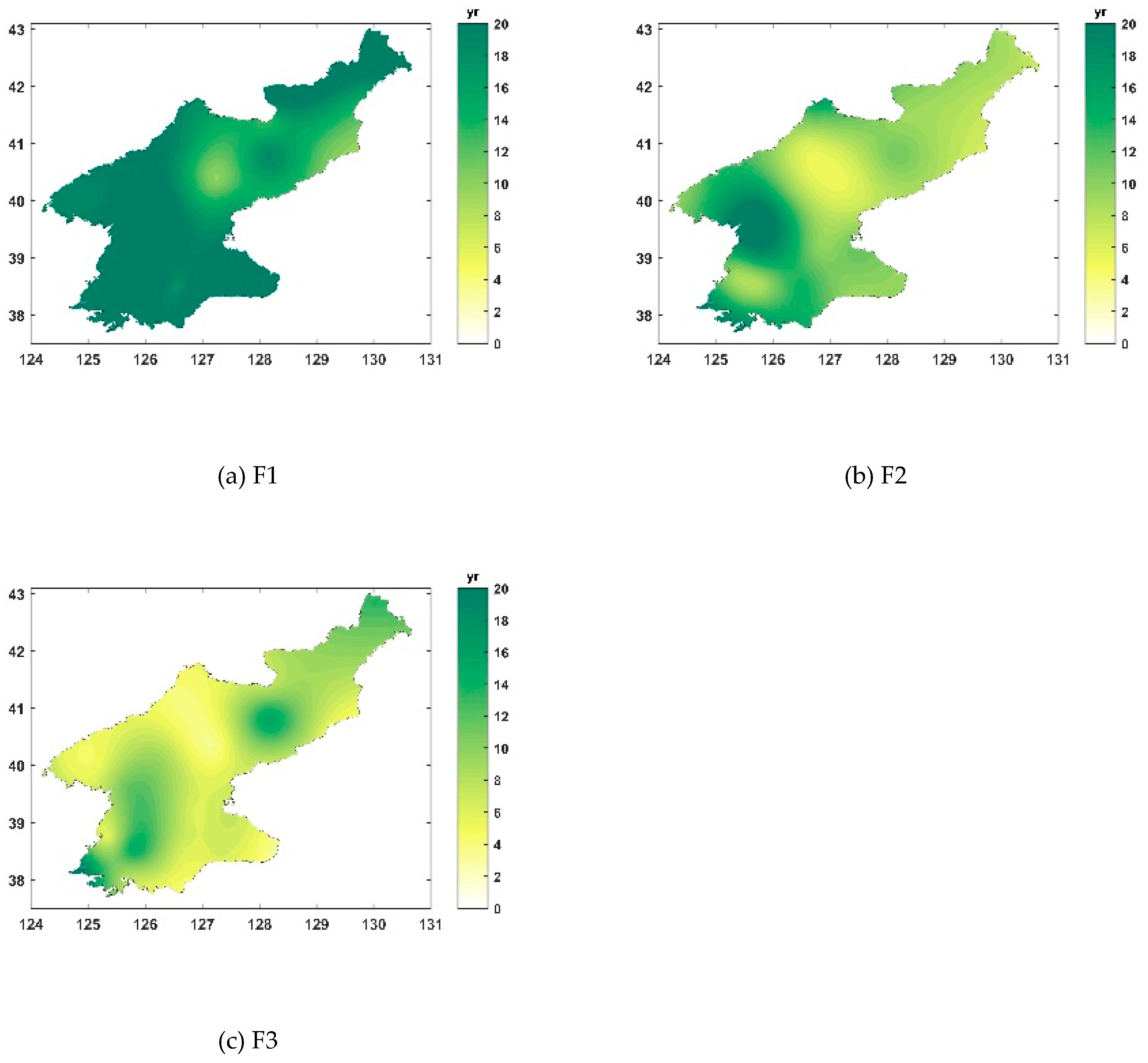
A non-stationarity was noticed in the 20-year precipitation frequency over time, and the 20-year return period in the current climate was expected to decrease in the future. Therefore, we projected the changed return periods for the 20-year frequency precipitation of the reference period (as shown in Figure 11). The spatially averaged return period in F1 was 20.7 years (Figure 11a), and climate change accelerated the return period to 11.7 years and 8.3 years in F2 and F3, respectively (as shown in Figure 11b,c). In particular, an extreme precipitation event in F3 was expected to occur every 4.4years in Changjon, located on the east coast of North Korea (Figure 11).
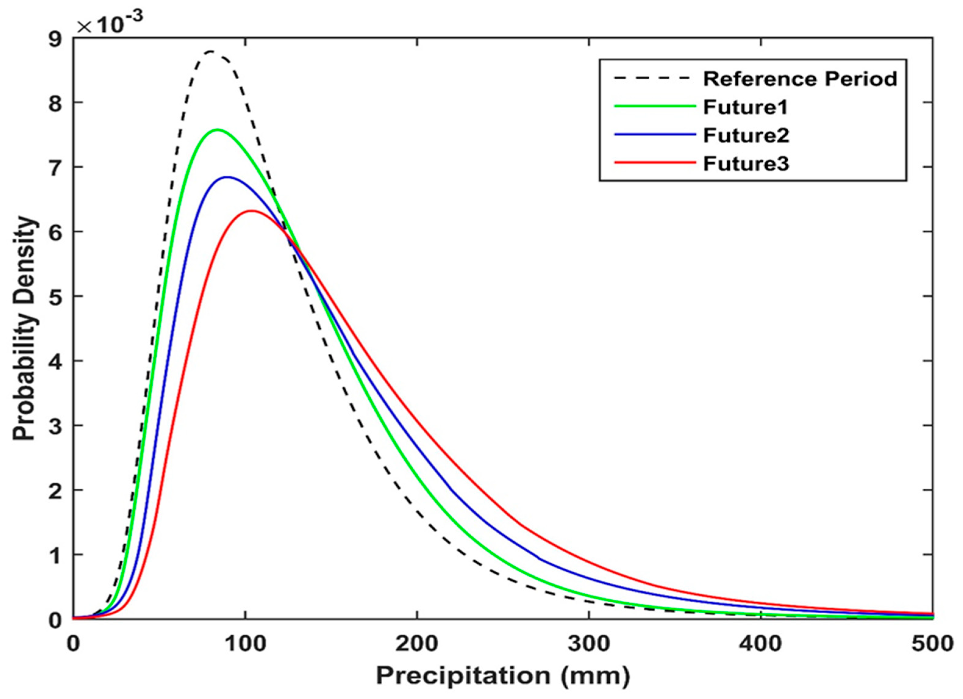
Generally, the PDF changes with time due to climate change, which means that the location and scale parameters of GEV distribution also increase over time, and the shape parameter becomes smaller [17]. Similar to previous studies, changes to the GEV parameters caused the location parameters from the present to F3 to increase from 93.5 to 127.0 and the scale parameters to increase from 35.0 to 50.2. The shape parameter decreased from −0.121 to −0.126. This means that the magnitude and frequency of extreme precipitation events would increase during future periods as compared to the reference period (as shown in Figure 12). The upper tail of GEV-PDF in the future would become thicker due to the decrease of the shape parameters, and therefore, the occurrence probability of extreme precipitation would increase.
5. Conclusions
The assessment of future changes in climate extremes has been challenging due to the intrinsic uncertainty associated with the use of different scales and mechanisms across a wide range of climate models. MME has been widely used for handling this uncertainty; meanwhile, the IPCC argued that likelihood of each model should be considered equally. Nonetheless, it is complicated and difficult to formulate decisions due to the large computational costs that arise in considering large numbers of climate change scenarios. Hence, this study selected the RCCS using the KKZ algorithm in order to assess the impact of climate change on extreme precipitation in North Korea. The selected RCCS were then evaluated by comparing with observation and all CCS. Finally, the magnitude and frequency of extreme precipitation in North Korea was projected for three future periods using RCCS. As a result, RCCS successfully retained the full range of variability and the same mean value across all months that was obtained by all CCS. The mean summer precipitation for North Korea as calculated from observation, all CCS, and RCCS was therefore 494, 533, and 536 mm, respectively.
Using RCCS for North Korea, extreme precipitation in North Korea was projected for three future periods. Compared to the present, although a slight decrease in extreme precipitation events was expected in F1, there was an increasing trend found in the magnitude and frequency of extreme precipitation from F1 through to F3. This is because the values of the location and scale parameters of GEV increase with projection further into the future. Moreover, since the value of the shape parameters displayed a decreasing trend, it was projected that the probability of occurrence of extreme precipitation events will increase in the future. When compared to previous study, Kwon et al. [41] and the current study both show consistent results, that is, 8.3 and 8.8 years for the return period of extreme precipitation under Kwon et al. [41] and the current study, respectively. Thus, the current study is able to deal with all the potential uncertainties arising from all the models by using only the RCCS, which is a subset of all the models.
There was a higher likelihood of extreme precipitation in Pyongyang, Singye, and Kaesong where are located near to the MDL. In these regions, extreme precipitation events have been caused mainly by mid-latitude cyclones approaching the Korean Peninsula, along with the enhanced Changma front supplying water vapor to the East China Sea. Lee et al. [43] indicated that these synoptic-scale features under current conditions are similar to those of future extreme events, using HadGEM3-RA simulations. Lee et al. [44] examined future changes in precipitation over Northeast Asia and Korea using five RCM simulations and indicated that extreme precipitation events are mainly associated with the southwest-to-northeast evolution of large-scale low-pressure systems in both current and future climates. The projected extreme precipitation events can cause frequent river erosion and sediment transport in these regions. The environmental impacts of sedimentation include loss of aquatic habitat, changes in fish migration, decrease in fishery resources, and so forth. There are also negative impacts of erosion, which include water pollution, siltation, and reduction in water storage capacity. Therefore, appropriate adaptive plans should be established. The recently announced policy about forest restoration would be one of them. Furthermore, in these regions, since the North-Han and Imjin River watersheds share both territories of South and North Korea, cooperative adaptation strategies to mitigate problems caused by future extreme precipitation should be established.
In this study, it is confirmed that the extreme precipitation obtained by the MME of the selected scenarios (RCCS) can fully account for all the scenarios (all CCS). The novelty of this study stems from the fact that there have been few studies addressing the impact of climate change with regards to extreme precipitation, although North Korea is known to be susceptible to significant threat from future climate change. Furthermore, it would be worth evaluating the future prospects of changes in flood volumes in North Korea, utilizing the RCCS.
Author Contributions
Conceptualization, J.H.S. and S.B.S.; Formal analysis, J.H.S. and M.K.; Funding acquisition, J.-J.J.; Investigation, J.-J.J.; Methodology, J.H.S. and S.B.S.; Software, M.K.; Supervision S.B.S.; Visualization, J.H.S.; Writing – original draft, J.H.S. and M.K.; Writing – review & editing, S.B.S.
Funding
This research was funded by the Ministry of Science, ICT and Future Planning, grant number NRF-2016R1C1B1010545, and The APC was funded by the Ministry of Science, ICT and Future Planning, grant number NRF-2016R1C1B1010545.
Acknowledgments
This research has been supported by a grant NRF-2016R1C1B1010545 funded by the Ministry of Science, ICT and Future Planning. The authors also thank Korea Environment Institute for their support.
Conflicts of Interest
The authors declare no conflict of interest.
References
- Lee, D.K.; Cha, D.H.; Kang, H.S. Regional climate simulation of the 1998 summer flood over East Asia. J. Meteorol. Soc. Jpn. 2004, 82, 1735–1753. [Google Scholar] [CrossRef]
- Kang, H.S.; Cha, D.H.; Lee, D.K. Evaluation of the mesoscale model/land surface model (MM5/LSM) coupled model for East Asian summer monsoon simulations. J. Geophys. Res.-Atmos. 2005, 110, D10105. [Google Scholar] [CrossRef]
- Hong, S.Y.; Lee, J.W. Assessment of the WRF model in reproducing a flash-flood heavy rainfall event over Korea. Atmos. Res. 2009, 93, 818–831. [Google Scholar] [CrossRef]
- Kim, Y.; Kang, B.; Adams, J.M. Opposite trends in summer precipitation in South and North Korea. Int. J. Climatol. 2012, 32, 2311–2319. [Google Scholar] [CrossRef]
- Sung, J.H.; Chung, E.-S.; Kim, Y.; Lee, B.R. Meteorological hazard assessment based on trends and abrupt changes in rainfall characteristics on the Korean peninsula. Theor. Appl. Climatol. 2017, 127, 305–326. [Google Scholar] [CrossRef]
- Harmeling, S.; Eckstein, D. Global Climate Risk Index 2013; Germanwatch: Bonn, Germany, 2012; ISBN 978-3-943704-04-4. [Google Scholar]
- Harmeling, S. Global Climate Risk Index 2009; Germanwatch: Bonn, Germany, 2008; ISBN 978-3-939846-45-1. [Google Scholar]
- Min, S.K.; Zhang, X.; Zwiers, F.W.; Hegerl, G.C. Human contribution to more-intense precipitation extremes. Nature 2011, 470, 378–381. [Google Scholar] [CrossRef]
- Kharin, V.V.; Zwiers, F.W.; Zhang, X.; Wehner, M. Changes in temperature and precipitation extremes in the CMIP5 ensemble. Clim. Chang. 2013, 119, 345–357. [Google Scholar] [CrossRef]
- Zhang, X.; Wan, H.; Zwiers, F.W.; Hegerl, G.C.; Min, S.K. Attributing intensification of precipitation extremes to human influence. Geophys. Res. Lett. 2013, 40, 5252–5257. [Google Scholar] [CrossRef] [Green Version]
- Fischer, E.M.; Knutti, R. Observed heavy precipitation increase confirms theory and early models. Nat. Clim. Chang. 2016, 6, 986–991. [Google Scholar] [CrossRef]
- Zhang, X.; Zwiers, F.W.; Li, G.; Wan, H.; Cannon, A.J. Complexity in estimating past and future extreme short-duration rainfall. Nat. Geosci. 2017, 10, 255–259. [Google Scholar] [CrossRef]
- Raftery, A.E.; Gneiting, T.; Balabdaoui, F.; Polakowski, M. Using Bayesian model averaging to calibrate forecast ensemble. Mon. Weather Rev. 2005, 133, 1155–1174. [Google Scholar] [CrossRef]
- Raisanen, J.; Palmer, T.N. A probability and decision-model analysis of a multimodel ensemble of climate change simulation. J. Clim. 2001, 14, 3212–3226. [Google Scholar] [CrossRef]
- Rajagopalan, B.; Lall, U.; Zebiak, S.E. Categorical climate forecasts through regularization and optimal combination of multiple GCM ensembles. Mon. Weather Rev. 2002, 130, 1792–1811. [Google Scholar] [CrossRef]
- Sung, J.H.; Chung, E.-S.; Shahid, S. Reliability–Resiliency–Vulnerability Approach for Drought Analysis in South Korea Using 28 GCMs. Sustainability 2018, 10, 3043. [Google Scholar] [CrossRef]
- Sung, J.H.; Eum, H.-I.; Park, J.; Cho, J. Assessment of Climate Change Impacts on Extreme Precipitation Events: Applications of CMIP5 Climate Projections Statistically Downscaled over South Korea. Adv. Meteorol. 2018, 2018, 4720523. [Google Scholar] [CrossRef]
- Seo, S.B.; Kim, Y.-O.; Kim, Y.; Eum, H.-I. Selecting climate change scenarios for regional hydrologic impact studies based on climate extremes indices. Clim. Dyn. 2019, 52, 1595–1611. [Google Scholar] [CrossRef]
- Seo, S.B.; Kim, Y.-O. Impact of Spatial Aggregation Level of Climate Indicators on a National-Level Selection for Representative Climate Change Scenarios. Sustainability 2018, 10, 2409. [Google Scholar] [CrossRef]
- Tebaldi, C.; Sanso, B. Joint projections of temperature and precipitation change from multiple climate models: A hierarchical Bayesian approach. J. R. Stat. Soc. Ser. C Appl. Stat. 2009, 172, 83–106. [Google Scholar] [CrossRef]
- Watterson, I.; Whetton, P. Joint PDFs for Australian climate in future decades and an idealized application to wheat crop yield. Aust. Meteorol. Ocean. 2011, 61, 221–230. [Google Scholar] [CrossRef]
- Luo, L.; Wood, E.F. Use of Bayesian merging techniques in a multimodel seasonal hydrologic ensemble prediction system for the eastern United States. J. Hydrometeorol. 2008, 9, 866–884. [Google Scholar] [CrossRef]
- Wang, H.; Reich, B.; Lim, Y.H. A Bayesian approach to probabilistic streamflow forecasts. J. Hydroinform. 2013, 15, 381–391. [Google Scholar] [CrossRef]
- Seo, S.B.; Kim, Y.-O.; Kang, S.-U.; Chun, G.I. Improvement in long-range streamflow forecasting accuracy using the Bayesian method. Hydrol. Res. 2019. [Google Scholar] [CrossRef]
- McSweeney, C.F.; Jones, R.G.; Lee, R.W.; Rowell, D.P. Selecting CMIP5 GCMs for downscaling over multiple regions. Clim. Dyn. 2015, 44, 3237–3260. [Google Scholar] [CrossRef]
- Lee, J.-K.; Kim, Y.-O. Selecting climate change scenarios reflecting uncertainties. Atmosphere 2012, 22, 149–161. [Google Scholar] [CrossRef]
- Knutti, R.; Masson, D.; Gettelman, A. Climate model genealogy: Generation CMIP5 and how we got there. Geophys. Res. Lett. 2013, 40, 1194–1199. [Google Scholar] [CrossRef] [Green Version]
- Molteni, F.; Buizza, R.; Marsigli, C.; Montani, A.; Nerozzi, F.; Paccagnella, T. A strategy for high-resolution ensemble prediction. I: Definition of representative members and global-model experiments. Q. J. R. Meteorol. Soc. 2001, 127, 2069–2094. [Google Scholar] [CrossRef]
- Houle, D.; Bouffard, A.; Duchesne, L.; Logan, T.; Harvey, R. Projections of future soil temperature and water content for three southern Quebec forested sites. J. Clim. 2012, 25, 7690–7701. [Google Scholar] [CrossRef]
- Katsavounidis, I.; Kuo, C.C.J.; Zhang, Z. A new initialization technique for generalized Lloyd iteration. IEEE Signal Process. Lett. 1994, 1, 144–146. [Google Scholar] [CrossRef]
- Cannon, A.J.; Sobie, S.R.; Murdock, T.Q. Bias Correction of GCM Precipitation by Quantile Mapping: How Well Do Methods Preserve Changes in Quantiles and Extremes? J. Clim. 2015, 28, 6938–6959. [Google Scholar] [CrossRef]
- Chen, J.; Brissette, F.P.; Lucas-Picher, P. Transferability of optimally-selected climate models in the quantification of climate change impacts on hydrology. Clim. Dyn. 2016, 47, 3359–3372. [Google Scholar] [CrossRef]
- Eum, H.-I.; Cannon, A.J. Intercomparison of projected changes in climate extremes for South Korea: Application of trend preserving statistical downscaling methods to the CMIP5 ensemble. Int. J. Climatol. 2017, 37, 3381–3397. [Google Scholar] [CrossRef]
- Cannon, A.J. Selecting GCM scenarios that span the range of changes in a multimodel ensemble: Application to CMIP5 climate extremes indices. J. Clim. 2015, 28, 1260–1267. [Google Scholar] [CrossRef]
- Katz, R.W.; Parlange, M.B.; Naveau, P. Statistics of extremes in hydrology. Adv. Water Resour. 2002, 25, 1287–1304. [Google Scholar] [CrossRef] [Green Version]
- Kharin, V.V.; Zwiers, F.W. Estimating extremes in transient climate change simulations. J. Clim. 2005, 18, 1156–1173. [Google Scholar] [CrossRef]
- Kharin, V.V.; Zwiers, F.W.; Zhang, X. Intercomparison of near surface temperature and precipitation extremes in AMIP-2 simulations, reanalyses, and observations. J. Clim. 2006, 18, 5201–5223. [Google Scholar] [CrossRef]
- Stedinger, J.R.; Vogel, R.M.; Foufoula-Georgiou, E. Chapter 18: Frequency Analysis of Extreme Events. In Handbook of Hydrology; Maidment, D.R., Ed.; McGraw-Hill: New York, NY, USA, 1993. [Google Scholar]
- Hosking, J.R.M.; Wallis, J.R. Regional Frequency Analysis: An Approach Based on L-Moments; Cambridge University Press: Cambridge, UK, 1997. [Google Scholar]
- Klein Tank, A.M.G.; Zwiers, F.W.; Zhang, X. Guidelines on Analysis of Extremes in a Changing Climate in Support of Informed Decisions for Adaptation; Climate Data and Monitoring WCDMP-No. 72, WMO-TD 2009; No. 1500; World Meteorological Organization: Geneva, Switzerland, 2009; 56p. [Google Scholar]
- Kwon, M.; Sung, J.H.; Ahn, J. Change in Extreme Precipitation over North Korea Using Multiple Climate Change Scenarios. Water 2019, 11, 270. [Google Scholar] [CrossRef]
- Kwon, M.; Sung, J.H. Changes in Future Drought with HadGEM2-AO Projections. Water 2019, 11, 312. [Google Scholar] [CrossRef]
- Lee, H.; Moon, B.-K.; Wie, J. Future extreme temperature and precipitation mechanisms over the Korean peninsula using a regional climate model simulation. J. Korean Earth Sci. Soc. 2018, 39, 327–341. [Google Scholar] [CrossRef]
- Lee, D.; Min, S.-K.; Jin, J.; Lee, J.-W.; Cha, D.-H.; Suh, M.-S.; Joh, M. Thermodynamic and dynamic contributions to future changes in summer precipitation over Northeast Asia and Korea: A multi-RCM study. Clim. Dyn. 2017, 49, 4121–4139. [Google Scholar] [CrossRef]
Figure 1.
The procedure utilized for this study.

Figure 2.
Weather stations in North Korea.

Figure 3.
Precipitation characteristics over North Korea.

Figure 4.
Simulated and observed monthly precipitation (All CCS, RCCS, FGOALS-s2, GFDL-ESM2G, HadGEM2-CC, CanESM2, IPSL-CM5A-MR and observation (mm/month)).
Figure 4.
Simulated and observed monthly precipitation (All CCS, RCCS, FGOALS-s2, GFDL-ESM2G, HadGEM2-CC, CanESM2, IPSL-CM5A-MR and observation (mm/month)).

Figure 5.
Difference between (a) all CSS, (b) RCCS, (c) FGOALS-s2, (d) GFDL-ESM2G, (e) HadGEM2-CC, (f) CanESM2, (g) IPSL-CM5A-MR and Observations in terms of 20-year return value of precipitation (unit: mm).
Figure 5.
Difference between (a) all CSS, (b) RCCS, (c) FGOALS-s2, (d) GFDL-ESM2G, (e) HadGEM2-CC, (f) CanESM2, (g) IPSL-CM5A-MR and Observations in terms of 20-year return value of precipitation (unit: mm).

Figure 6.
GEV-PDF of All CCS, RCCS, FGOALS-s2, GFDL-ESM2G, HadGEM2-CC, CanESM2, IPSL-CM5A-MR, and Observation for reference period.
Figure 6.
GEV-PDF of All CCS, RCCS, FGOALS-s2, GFDL-ESM2G, HadGEM2-CC, CanESM2, IPSL-CM5A-MR, and Observation for reference period.

Figure 7.
Difference between RCCS, five scenarios of RCCS and all CCS for 20-year frequency of extreme precipitation (unit: mm).
Figure 7.
Difference between RCCS, five scenarios of RCCS and all CCS for 20-year frequency of extreme precipitation (unit: mm).

Figure 8.
Difference between RCCS, five scenarios of RCCS, and all CCS in the return period (unit: years).
Figure 8.
Difference between RCCS, five scenarios of RCCS, and all CCS in the return period (unit: years).

Figure 9.
GEV-PDF of All CCS (grey envelop), RCCS (5 scenarios), FGOALS-s2, GFDL-ESM2G, HadGEM2-CC, CanESM2, IPSL-CM5A-MR for F3 period, and observation for reference period (current).
Figure 9.
GEV-PDF of All CCS (grey envelop), RCCS (5 scenarios), FGOALS-s2, GFDL-ESM2G, HadGEM2-CC, CanESM2, IPSL-CM5A-MR for F3 period, and observation for reference period (current).

Figure 10.
Projection of changes in 20-year return value of precipitation based on RCCS (unit: mm).

Figure 11.
Change in 20-year return period of AMDP for 25 CMIP5 GCMs for the F1, F2, and F3 periods under RCP8.5. (a) F1 under RCP8.5, (b) F2 under RCP8.5, and (c) F3 under RCP8.5 (unit: years).
Figure 11.
Change in 20-year return period of AMDP for 25 CMIP5 GCMs for the F1, F2, and F3 periods under RCP8.5. (a) F1 under RCP8.5, (b) F2 under RCP8.5, and (c) F3 under RCP8.5 (unit: years).

Figure 12.
Changes in GEV-PDF for F1 (Future1), F2 (Future2), and F3 (Future3) period comparing to RCCS of current period (Reference Period).
Figure 12.
Changes in GEV-PDF for F1 (Future1), F2 (Future2), and F3 (Future3) period comparing to RCCS of current period (Reference Period).


Table 1.
25 GCMs from CMIP5 used for this study.
| No. | GCMs | Resolution (degree) | Institution |
|---|---|---|---|
| 1 | CanESM2 | 2.813 × 2.791 | Canadian Centre for Climate Modelling and Analysis |
| 2 | CCSM4 | 1.250 × 0.942 | National Center for Atmospheric Research |
| 3 | CESM1-BGC | 1.250 × 0.942 | |
| 4 | CESM1-CAM5 | 1.250 × 0.942 | |
| 5 | CMCC-CM | 0.750 × 0.748 | Centro Euro-Mediterraneo per I Cambiamenti Climatici |
| 6 | CMCC-CMS | 1.875 × 1.865 | |
| 7 | CNRM-CM5 | 1.406 × 1.401 | Centre National de Recherches Meteorologiques |
| 8 | CSIRO-Mk3-6-0 | 1.875 × 1.865 | Commonwealth Scientific and Industrial Research Organisation and Queensland Climate Change Center of Excellence |
| 9 | FGOALS-g2 | 2.791 × 2.813 | LASG, Institute of Atmospheric Physics, Chinese Academy of Sciences |
| 10 | FGOALS-s2 | 2.813 × 1.659 | |
| 11 | GFDL-CM3 | 2.500 × 2.000 | Geophysical Fluid Dynamics Laboratory |
| 12 | GFDL-ESM2G | 2.000 × 2.023 | |
| 13 | GFDL-ESM2M | 2.500 × 2.023 | |
| 14 | HadGEM2-AO | 1.875 × 1.250 | Met Office Hadley Centre |
| 15 | HadGEM2-CC | 1.875 × 1.250 | |
| 16 | INM-CM4 | 2.000 × 1.500 | Institute for Numerical Mathematics |
| 17 | IPSL-CM5A-LR | 3.750 × 1.895 | Institute Pierre-Simon Laplace |
| 18 | IPSL-CM5A-MR | 2.500 × 1.268 | |
| 19 | IPSL-CM5B-LR | 3.750 × 1.895 | |
| 20 | MIROC-ESM | 2.813 × 2.791 | Japan Agency for Marine-Earth Science and Technology |
| 21 | MIROC-ESM-CHEM | 2.813 × 2.791 | |
| 22 | MPI-ESM-LR | 1.875 × 1.865 | Max Planck Institute for Meteorology (MPI-M) |
| 23 | MPI-ESM-MR | 1.875 × 1.865 | |
| 24 | MRI-CGCM3 | 1.125 × 1.122 | Meteorological Research Institute |
| 25 | NorESM1-M | 2.500 × 1.895 | Norwegian Climate Centre |
Table 2.
Generalized Extreme Value (GEV) parameters of each scenario for the reference period.
| Data | GEV Parameter | ||
|---|---|---|---|
| Location | Scale | Shape | |
| Observation | 80.618 | 28.585 | −0.107 |
| All CCS | 95.510 | 36.541 | −0.092 |
| FGOALS−s2 | 92.094 | 34.936 | −0.177 |
| GFDL-ESM2G | 91.938 | 38.509 | −0.107 |
| HadGEM2-CC | 94.081 | 33.118 | −0.060 |
| CanESM2 | 93.565 | 32.818 | −0.173 |
| IPSL-CM5A-MR | 95.620 | 35.775 | −0.112 |
| RCCS | 93.460 | 35.031 | −0.126 |
© 2019 by the authors. Licensee MDPI, Basel, Switzerland. This article is an open access article distributed under the terms and conditions of the Creative Commons Attribution (CC BY) license (http://creativecommons.org/licenses/by/4.0/).
Share and Cite
MDPI and ACS Style
Sung, J.H.; Kwon, M.; Jeon, J.-J.; Seo, S.B. A Projection of Extreme Precipitation Based on a Selection of CMIP5 GCMs over North Korea. Sustainability 2019, 11, 1976. https://0-doi-org.brum.beds.ac.uk/10.3390/su11071976
AMA Style
Sung JH, Kwon M, Jeon J-J, Seo SB. A Projection of Extreme Precipitation Based on a Selection of CMIP5 GCMs over North Korea. Sustainability. 2019; 11(7):1976. https://0-doi-org.brum.beds.ac.uk/10.3390/su11071976
Chicago/Turabian StyleSung, Jang Hyun, Minsung Kwon, Jong-June Jeon, and Seung Beom Seo. 2019. "A Projection of Extreme Precipitation Based on a Selection of CMIP5 GCMs over North Korea" Sustainability 11, no. 7: 1976. https://0-doi-org.brum.beds.ac.uk/10.3390/su11071976
Note that from the first issue of 2016, this journal uses article numbers instead of page numbers. See further details here.