A Stochastic Differential Game in the Closed-Loop Supply Chain with Third-Party Collecting and Fairness Concerns

Abstract

This paper investigates the optimal return control problem in a closed-loop supply chain consisted of one manufacturer, one retailer, and one third-party collector, in the presence of stochastic return disturbance and fairness concern of followers. We formulate the stochastic differential game-theoretic models and resolve the feedback Stackelberg equilibriums without and with fairness concern. We also derive the evolutionary paths of the stochastic return rate and the value functions of the supply chain members under the optimal control strategies. We find that the feedback equilibrium exists only under a specific condition, and the expectation and variance of the return rate both approach the stable state for a specific closed-loop supply chain system. We further discussed the impact of fairness concerns on the supply chain system. The manufacturer would shift profit to the retailer by lowering the wholesale price, and the stable expected return rate will be lower in the supply chain with fairness concerns, as the third party will have less incentive to collect used products, considering unfairness. The manufacturer should set a higher transfer subsidy to incentivize the third party to collect when the third party is concerned with fairness.

1. Introduction

Remanufacturing of used products is cost saving for the manufacturers and is thus adopted by more and more manufacturers [1], e.g., HP, Lenovo, Apple, and Xerox [2,3]. However, collection activities involve complexity and uncertainty because of the long distance of the supply chain, the broad area of the used-product distribution, and uncertainty of product quality [4,5,6]. Therefore, how to collect used products in the presence of stochastic disturbance is an essential problem for the manufacturers.

In practice, third-party collection is widely used by manufacturers to gather their used products. For example, the ‘big three’ auto manufacturers (i.e., General Motors, Ford, and Chrysler) started to cooperate with third parties on used-product collection and remanufacturing [7]. Third parties usually serve as a maintenance service provider or waste products recycler. As a result, they have the advantage of a better chance to come into contact with end customers who may have used products to dispose of, which makes third-party collection an effective way to collect used products. On the other hand, more and more studies are considering that the decision members in the supply chain are concerned with fairness [8,9,10], especially the followers in the supply chain. Thus, we want to investigate how the followers’ concerns about fairness would affect the optimal return strategies in a closed-loop supply chain.

In the area of closed-loop supply chains, most of the existing studies [2,11] adopted the static formulation of return rate, which ignored the dynamic characteristic of the return rate with collection efforts. However, most of the collecting activities, such as return advertising, collecting facilities maintenance, and reverse logistics establishing, are marketing-type activities which have dynamic characteristics and long-term effects, i.e., the system state depends on the whole efforts accumulation and not just on the current effort level [6,12,13]. To investigate the used-product return problem in the dynamic setting, we develop a stochastic differential game in a supply chain which consisted of one manufacturer, one retailer, and one third-party collector. This study aims to formulate the dynamic model of a closed-loop supply chain with third-party collection and then resolve the Stackelberg equilibrium and optimal collection control strategies for the supply chain members in the presence of the stochastic disturbance.

In a closed-loop supply chain, the supply chain members are usually formulated as rational in their payoffs and do not care about others’ payoffs. However, more and more researchers are arguing that the players may be concerned about fairness, especially in the supply chain with one leader and several followers [14,15]. The Stackelberg leader in the supply chain may take a large proportion of the revenue from the system, which results in feelings of unfairness for the followers. This study wants to incorporate the concept of fairness concern into the third-party collection closed-loop supply chain and discuss how the presence of fairness concerns would affect the equilibrium and profitability for the supply chain members.

Given the importance of remanufacturing closed-loop supply chain, lots of studies have dealt with the operation, pricing, and return problem of a closed-loop supply chain. We refer to Atasu et al. [16], Govindan et al. [17], and Govindan and Soleimani [18] for comprehensive reviews of closed-loop supply chain operations.

The reverse-channel management is a critical issue in closed-loop supply chain management. Savaskan et al. [11] utilized the game theory to formulate the reverse-channel design problem in the closed-loop supply chain, i.e., manufacturer collecting channel, retailer collecting channel, and third-party collecting channel. They found that the reverse channel with retailer collecting might be the optimal reverse channel for a closed-loop supply chain. Savaskan and Van Wassenhove [2] further considered the reverse-channel design problem in the scenario of competing retailers. Huang et al. [19] examined a CLSC with a dual recycle channel in which the manufacturer sells products via the retailer in the forward chain, while the retailer and the third party simultaneously collect used products in the reverse channel. De Giovanni and Zaccour [20] studied the collection outsourcing choice of the manufacturer in a CLSC, where the retailer or the third-party firm can undertake the outsourcing task. These papers focused on the reverse-channel management problem with a single supply chain member take the collection activities in the supply chain.

Some researchers have considered the co-operation of used-products return problem across the supply chain members. Subramanian et al. [21] studied the effect of extended producer responsibility (EPR) on a remanufacturing supply chain. Jacobs and Subramanian [22] also considered the EPR programs, and they attempted to share the EPR responsibility within the supply chain. Jena and Sarmah [23] and Ma et al. [7] have investigated the co-operation problems in the competing scenarios in the closed-loop supply chain. These papers mainly focused on improving the collection efficiency by co-operation across the supply chain members.

The above papers are static return model-based, which ignores the dynamic characteristics in the return activities. Some studies have begun to discuss the used-product collection problem with dynamic models. Guide and Wassenhove [24] considered the used-product collection problem in the face of uncertain quality. Nakashima et al. [25] studied the optimal control problem in remanufacturing systems. Fallah et al. [26] studied the competition between two closed-loop supply chains in an uncertain environment. These papers mainly focused on the issues of product collection in terms of quality or timing uncertainty.

Regarding the dynamic return problems, De Giovanni and Zaccour [27], De Giovanni et al. [12], and Huang et al. [6] have developed the differential game model to formulate the return dynamics and discuss the optimal return control problems in decentralized supply chains. De Giovanni and Zaccour [27] formulated the differential game of a closed-loop supply chain and resolved the feedback equilibrium as well as the cost and revenue-sharing contract. De Giovanni et al. [12] further developed their model and examined the dynamic incentive strategies across the CLSC members to increase the return rate for the system. Huang et al. [6] formulated the stochastic differential game and derived the feedback equilibrium with manufacturer collection in the supply chain. These papers mainly focus on the optimal control strategy for a closed-loop supply chain. As best as we know, there is no existing research which has discussed the optimal return control problem for a third-party collection closed-loop supply chain system. Our study contributes to this area of literature by investigating the optimal control strategy and discussing the impact of fairness concerns for a third-party collection closed-loop supply chain.

There is an increasing number of studies focusing on the topic of fairness concerns in the supply chain management area during the past decade. Cui et al. [15] investigated how fairness may affect channel coordination in a dyadic supply chain. Du et al. [28] dealt with the newsvendor problem for a dyadic supply chain where both manufacturer and retailer have the preference of status-seeking with fairness concerns. Nie and Du [10] further considered the quantity discount contracts with dual-fairness in the supply chain. Ho et al. [29] discussed the contact design problem in the supply chain with two retailers with peer-induced fairness. These papers mainly focus on the impact of fairness on a general supply chain and how to coordinate the supply chain with fairness concern. Our study contributes to this area by incorporating the concept of fairness into the closed-loop supply chain and dealing with the impact of fairness concerns for the followers on the equilibrium and profitability for the supply chain members.

The existing studies tend to focus on either closed-loop supply or fairness concerns in the supply chain. Especially in the area of dynamic closed-loop supply chain management, there are few researchers who investigated the optimal return problem in the presence of fairness concern. In this paper, we deal with the stochastic optimal return control problem in a closed-loop supply chain with third-party collection. We derive the feedback equilibrium for the stochastic differential game and the evolutionary path of the return rate. Furthermore, we study the impact of fairness concerns on the third-party collection closed-loop supply chain. Specifically, we attempt to answer the following questions:

(1)

What is the equilibrium strategy for a third-party collection closed-loop supply chain system considering the random disturbance in the return process?

(2)

How would the presence of fairness concerns for the followers affect the equilibrium strategy as well as the profits for the supply chain members?

Our main results are as follows. First, we found that the feedback equilibrium exists only under a specific condition, and the expectation and variance of the return rate both approach the stable state. The monotonicity of the expectation and variance of the return rate is relevant to the initial value of the return rate. Second, the presence of fairness concerns for the followers in the supply chain would not change the equilibrium strategy for the retailer but do change strategies for the manufacturer and the third party. The manufacturer would shift profit to the retailer by lowering the wholesale price, and the stable expected return rate will be lower in the supply chain with fairness concerns, as the third party will have less incentive to collect used products considering the unfairness.

The remainder of this paper is organized as follows. Section 2 presents our modeling framework. Section 3 resolves the feedback equilibrium of the stochastic differential game presented in Section 2. Section 4 is the numerical analysis of the stochastic return rate and profitability of supply chain members. Section 5 extends the model into the scenario with fairness concerns of followers and derives the corresponding feedback equilibrium. Section 6 concludes the paper.

2. The Model

We consider a closed-loop supply chain system, which consists of one manufacturer, one retailer, and one third-party collector. The manufacturer distributes its products through the retailer and collects the used products from the consumers by the third-party collector. The unit production cost for the manufacturer is $c_m$ when only the raw material is used to make the new product. The manufacturer can also make use of the used products for manufacturing the new product, with a unit production cost $c_r$. We assume $c_r<c_m$, which means that the remanufacturing is cost saving; otherwise, the manufacturer would not utilize the remanufacturing technique. Denote $\mathsf{\Delta }=c_m-c_r$ as the unit cost savings by remanufacturing the used product. We consider the case where the products made from new raw materials as well as used products are entirely the same, which means the manufacturer uses the used products as production materials; the case where the products made by the new raw materials and the used products are differentiated in some dimensions is beyond the scope of this paper.

Time $t$ is continuous, and the planning horizon for the decision makers is $t\in [0, \infty )$. $R\left(t\right)$ denotes the return rate of used products from the consumers at time $t$, which represents the percentage of used products collected from the consumers by the third party and also represents the percentage of product made by used products as materials for the manufacturer. $E\left(t\right)$ denotes the collecting efforts of the third party at time $t$, which indicates the efforts that the third party invests in collection activities, such as collection advertising, collection facilities, and reverse logistics. We follow the setting in De Giovanni and Zaccour [27] and Huang et al. [6], i.e., the return rate $R\left(t\right)$ depends on the whole history of collection efforts, formulating the return rate by the Itô equation as

$$\begin{array}{c}dR\left(t\right)=\left(\theta E\left(t\right)-\delta R\left(t\right)\right)dt+\sigma \left(R\left(t\right)\right)dz\left(t\right),R\left(t\right)=R_0\ge 0\end{array}$$

(1)

where $\theta$ represents the impact of collecting efforts on the return rate; $\delta$ measures the decaying rate of the dynamic system, which indicates the rate that the consumers forget about the returning policy or the wearing of the return facilities. $R_0\in \left[0,1\right]$ represents the initial return rate of the closed-loop supply chain system. $\sigma \left(R\left(t\right)\right)$ is a variance term and $z\left(t\right)$ is a standard Wiener process. The term $\left(\theta E\left(t\right)-\delta R\left(t\right)\right)dt$ is deterministic and represents the net influence of collecting effort on the return rate, while the term $\sigma \left(R\left(t\right)\right)dz\left(t\right)$ is indeterminate and represents the stochastic disturbance of the random factors on the return rate. Equation (1) captures the dynamics in the collecting process in the closed-loop supply chain system, which shows the dynamic return rate is impacted by three parts, i.e., collecting efforts, system decaying and the stochastic disturbance.

The return rate must satisfy $0\le R\le 1$. Therefore, $E$ and $\sigma \left(R\right)$ should be continuous functions, and they should satisfy the Lipschitz conditions on each closed subinterval of $\left(0,1\right)$. Moreover, $E\left(R\right)\ge 0$ when $R\in \left[0,1\right]$, and $\sigma \left(R\right)>0$ when $R\in \left(0,1\right)$ and $\sigma \left(0\right)=0$. With this condition, the drift at $R=0$ is positive as long as $\theta E\left(0\right)-\delta R\left(0\right)>0$, which can be met easily when $R\left(0\right)$ is small enough. Similar to Prasad and Sethi [30] and Huang et al. [6], we will adopt $\sigma \left(R\right)=\sigma \sqrt{R}$ to reduce the mathematical complexity.

The manufacturer is the Stackelberg leader in the supply chain system, and the retailer and third party are followers. The manufacturer announces the wholesale price $\omega \left(t\right)$ and distributes new products to the retailer, and then the retailer sets the retailer price $p\left(t\right)$ and sells new products to the consumers; in the meantime, the third-party collector will decide its collecting efforts $E\left(t\right)$ to collect used products from the hands of consumers and transfer to the manufacturer for remanufacturing, with unit return subsidy $s$. The cost function of the third-party for investing in collecting activities is assumed by $k{E}^2\left(t\right)/2$, where $k>0$ is a scaling parameter which represents the complexity degree for the third-party to collect used products. Denote the $A$ as the fixed payment given to the consumer for the third-party to collect a used product. Without loss of generality, we assume $A=0$ for the sake of simplicity.

Denote by $D\left(t\right)$ the demand of the retailer at time $t$. We adopt the classic demand function in the economics and management literature, which is given by

$$\begin{array}{c}D\left(t\right)=a-bp\left(t\right)\end{array}$$

(2)

where $a$ represents the market potential of the product, and $b$ measures the price sensitivity in the market.

The discount rate for the supply chain members is $\rho$. Denote $J_i\left(i=m,r,3p\right)$ as the profit function for player $i$ in the supply chain, where $m,r,3p$ represents the manufacturer, retailer, and third party, respectively. The objective function of the manufacturer is formulated as

$$\begin{array}{c}\underset{\omega \left(t\right)\ge 0}{\max }\left\{J_m^{}=\mathrm{E}{{\displaystyle \int }}_0^{\infty }{e}^{-\rho t}\left[\left(\omega \left(t\right)-c+\mathsf{\Delta }R\left(t\right)\right)D\left(t\right)-sR\left(t\right)D\left(t\right)\right]dt\right\}.\end{array}$$

(3)

The objective function of the retailer is formulated as

$$\begin{array}{c}\underset{p\left(t\right)\ge 0}{\max }\left\{J_r^{}=\mathrm{E}{{\displaystyle \int }}_0^{\infty }{e}^{-\rho t}\left[\left(p\left(t\right)-\omega \left(t\right)\right)D\left(t\right)\right]dt\right\}.\end{array}$$

(4)

The third-party maximizes the objective function in the following:

$$\begin{array}{c}\underset{E\left(t\right)\ge 0}{\max }\left\{J_{3p}^{}=\mathrm{E}{{\displaystyle \int }}_0^{\infty }{e}^{-\rho t}\left[sR\left(t\right)D\left(t\right)-\frac{1}{2}k{E}^2\left(t\right)\right]dt\right\}.\end{array}$$

(5)

The supply chain members seek to maximize their expected discounted profit stream subject to the system dynamics in Equation (1). The Hamilton–Jacobi–Bellman (HJB) equation method will be used to resolve the stochastic differential game presented above.

3. Equilibrium Analysis

We will resolve the feedback Stackelberg equilibrium of the differential game formulated in the previous section, and then characterize the evolutionary path of the system return rate.

3.1. Feedback Stackelberg Equilibrium

The manufacturer first announces its wholesale price control strategy $\omega \left(t\right)$, and then the retailer and the third-party decide their retail price control strategy $p\left(t\right)$ and collecting efforts $E\left(t\right)$, respectively. Denote $V_i\left(i=m,r,3p\right)$ as the value functions of the supply chain member, and the Hamilton–Jacobi–Bellman equations of the retailer and the third-party are formulated by

$$\begin{array}{c}\rho V_r^{}=\underset{p}{\max }\left\{\left(p-\omega \right)D+V_r^{\prime }\left(R\right)\left(\theta E-\delta R\right)+\frac{{\sigma }^2}{2}R{V}_r^{\prime \prime }\left(R\right)\right\},\end{array}$$

(6)

$$\begin{array}{c}\rho V_{3p}^{}=\underset{E}{\max }\left\{sRD-\frac{1}{2}k{E}^2+V_{3p}^{\prime }\left(R\right)\left(\theta E-\delta R\right)+\frac{{\sigma }^2}{2}R{V}_{3p}^{\prime \prime }\left(R\right)\right\},\end{array}$$

(7)

where $V_i^{\prime }=d{V}_r^{}/dR$ and $V_r^{\prime \prime }=d^2{V}_r^{}/d{R}^2$, $i=m,r,3p$. Thus, the best response of the retailer and third party can be resolved as

$$\begin{array}{c}p\left(\omega ,R\right)=\frac{a+b\omega }{2b}, E\left(R\right)=\frac{\theta }{k}{V}_{3p}^{\prime }\left(R\right).\end{array}$$

(8)

It is shown in Equation (8) that the collecting effort is irrelevant to the strategy of the manufacturer, and only related to the marginal value of the return rate of the third party. The HJB equation of the manufacturer can be formulated by

$$\begin{array}{c}\rho V_m^{}=\underset{\omega }{\max }\left\{\left(\omega -c+\mathsf{\Delta }R\right)D-sRD+V_m^{\prime }\left(R\right)\left(\theta E-\delta R\right)+\frac{{\sigma }^2}{2}R{V}_m^{\prime \prime }\left(R\right)\right\}.\end{array}$$

(9)

Inserting the best responses of the retailer and third party into the value function of the manufacturer and maximizing the HJB function of the manufacturer yields the optimal feedback wholesale price control strategy

$$\begin{array}{c}{\omega }^{*}\left(R\right)=\frac{a+b\left(c-\left(\mathsf{\Delta }-s\right)R\right)}{2b}.\end{array}$$

(10)

Taking back into the response function can obtain the optimal feedback retail price control strategy

$$\begin{array}{c}{p}^{*}\left(R\right)=\frac{3a+b\left(c-\left(\mathsf{\Delta }-s\right)R\right)}{4b}, E^{*}\left(R\right)=\frac{\theta }{k}{V}_{3p}^{\prime }\left(R\right).\end{array}$$

(11)

The term $c-\left(\mathsf{\Delta }-s\right)R$ reflects the real unit production of the manufacturer, which decreases with the return rate and increases with the transfer subsidy. Substituting the optimal control strategies into the value functions of the supply chain members, we find that the value functions are quadratic according to the return rate. As a result, we conjecture the value functions of the supply chain members as follows,

$$\begin{array}{c}\{\begin{array}{c}{V}_{3p}^{}=e_0+e_{1}R+e_2{R}^2,\\ V_r^{}=f_0+f_{1}R+f_2{R}^2,\\ V_m^{}=g_0+g_{1}R+g_2{R}^2.\end{array}\end{array}$$

(12)

where $e_j$, $f_j$, and $g_j$ $\left(j=0,1,2\right)$ are undetermined coefficients. Taking Equation (12) and their derivations into the value functions $V_i\left(p^{*}\left(R\right),{\omega }^{*}\left(R\right), E^{*}\left(R\right)\right)$ $\left(i=m,r,3p\right)$, we can obtain the coefficients equations that are to be solved,

$$\begin{array}{c}\{\begin{array}{c}\rho e_0=\frac{{\theta }^2}{2k}{e}_1{}^2,\hfill \\ \rho e_1=\frac{1}{4}s\left(a-bc\right)+e_1\left(\frac{2{\theta }^2}{k}{e}_2-\delta \right)+{\sigma }^2{e}_2\hfill \\ \rho e_2=\frac{1}{4}bs\left(\mathsf{\Delta }-s\right)+\frac{2{\theta }^2}{k}{e}_2{}^2-2\delta e_2,\hfill \end{array},\hfill \\ \{\begin{array}{c}\rho f_0=\frac{1}{16b}{\left(a-bc\right)}^2+\frac{{\theta }^2}{k}{e}_1{f}_1,\hfill \\ \rho f_1=\frac{1}{8}\left(a-bc\right)\left(\mathsf{\Delta }-s\right)+f_1\left(\frac{2{\theta }^2}{k}{e}_2-\delta \right)+\frac{2{\theta }^2}{k}{f}_2{e}_1+f_2{\sigma }^2,\hfill \\ \rho f_2=\frac{1}{16}b{\left(\mathsf{\Delta }-s\right)}^2+2f_2\left(\frac{2{\theta }^2}{k}{e}_2-\delta \right),\hfill \end{array}\hfill \\ \{\begin{array}{c}\rho g_0=\frac{1}{8b}{\left(a-bc\right)}^2+\frac{{\theta }^2}{k}{e}_1{g}_1,\hfill \\ \rho g_1=\frac{1}{4}\left(\mathsf{\Delta }-\mathrm{s}\right)\left(a-bc\right)+g_1\left(\frac{2{\theta }^2}{k}{e}_2-\delta \right)+\frac{2{\theta }^2}{k}{e}_1{g}_2+{\sigma }^2{g}_2,\hfill \\ \rho g_2=\frac{1}{8}b{\left(\mathsf{\Delta }-s\right)}^2+2g_2\left(\frac{2{\theta }^2}{k}{e}_2-\delta \right).\hfill \end{array}\hfill \end{array}$$

Denote ${\theta }_k={\theta }^2/2k$, $A=a-bc$, ${\mathsf{\Delta }}_s=\mathsf{\Delta }-s$, and the coefficients are solved by

$$\begin{array}{c}\{\begin{array}{c}\begin{array}{c}{e}_0=\frac{{\theta }_k}{\rho }{e}_1{}^2,\hfill \\ e_1=\frac{sA+4{\sigma }^2{e}_2}{4\left[\rho +\delta -4{\theta }_k{e}_2\right]},\hfill \\ e_2=\frac{\rho +2\delta \pm \sqrt{{\left(\rho +2\delta \right)}^2-4{\theta }_{k}bs{\mathsf{\Delta }}_s}}{8{\theta }_k},\hfill \end{array}\end{array}\end{array}\{\begin{array}{c}\begin{array}{c}{f}_0=\frac{1}{\rho }\left(\frac{A^2}{16b}+2{\theta }_k{e}_1{f}_1\right),\hfill \\ f_1=\frac{{\mathsf{\Delta }}_{s}A+32{\theta }_k{e}_1{f}_2+8{\sigma }^2{f}_2}{8\left[\rho +\delta -4{\theta }_k{e}_2\right]},\hfill \\ f_2=\frac{b{\mathsf{\Delta }}_s{}^2}{16\left(\rho +2\delta -8{\theta }_k{e}_2\right)},\hfill \end{array}\end{array}\{\begin{array}{c}\begin{array}{c}{g}_0=\frac{1}{\rho }\left(\frac{A^2}{8b}+2{\theta }_k{e}_1{g}_1\right),\hfill \\ g_1=\frac{{\mathsf{\Delta }}_{s}A+16{\theta }_k{e}_1{g}_2+4{\sigma }^2{g}_2}{4\left[\rho +\delta -4{\theta }_k{e}_2\right]}\hfill \\ g_2=\frac{b{\mathsf{\Delta }}_s{}^2}{8\left(\rho +2\delta -8{\theta }_k{e}_2\right)}.\hfill \end{array}\end{array}$$

(13)

Assume ${\left(\rho +2\delta \right)}^2-4{\theta }_{k}bs{\mathsf{\Delta }}_s>0$ to make sure $e_2$ is real. When $e_2=\frac{\rho +2\delta +\sqrt{{\left(\rho +2\delta \right)}^2-4{\theta }_{k}bs{\mathsf{\Delta }}_s}}{8{\theta }_k}$, $\rho +\delta -4{\theta }_k{e}_2=\frac{\rho -\sqrt{{\left(\rho +2\delta \right)}^2-4{\theta }_{k}bs{\mathsf{\Delta }}_s}}{2}$ needs to be positive, otherwise if $\rho +\delta -4{\theta }_k{e}_2<0$, $e_1$ will be negative; from $E^{*}=\frac{\theta }{k}\left(2e_{2}R+e_1\right)$ we can infer that there would be some small return rate values which make $E^{*}<0$ when $e_1<0$. However, $\rho +\delta -4{\theta }_k{e}_2>0$ means $\rho -\sqrt{{\left(\rho +2\delta \right)}^2-4{\theta }_{k}bs{\mathsf{\Delta }}_s}>0$, i.e., ${\theta }_{k}bs{\mathsf{\Delta }}_s>\delta \left(\rho +\delta \right)$. That is to say, $\theta >\sqrt{2k\delta \left(\rho +\delta \right)/bs{\mathsf{\Delta }}_s}$ or $k<{\theta }^{2}bs{\mathsf{\Delta }}_s/\left(2\delta \left(\rho +\delta \right)\right)$. However, this is counterintuitive as we always deem that the impact of collecting efforts should be small and the cost coefficient should be large. Therefore, we assume ${\theta }_{k}bs{\mathsf{\Delta }}_s<\delta \left(\rho +\delta \right)$ to exclude the larger root. When $e_2=\frac{\rho +2\delta -\sqrt{{\left(\rho +2\delta \right)}^2-4{\theta }_{k}bs{\mathsf{\Delta }}_s}}{8{\theta }_k}$, one can easily verify that $e_1>0$, and $E^{*}>0, \forall R\in \left[0,1\right]$.

Proposition 1.

When${\theta }_k< \raisebox{1ex}{$\delta \left(\rho +\delta \right)$}\!\left/ \!\raisebox{-1ex}{$bs{\mathsf{\Delta }}_s$}\right.$, there exists only one feedback Stackelberg Markov equilibrium. The equilibrium control strategies are given by

$${\omega }^{*}\left(R\right)=\frac{a+b\left(c-\left(\mathsf{\Delta }-s\right)R\right)}{2b},p^{*}\left(R\right)=\frac{3a+b\left(c-\left(\mathsf{\Delta }-s\right)R\right)}{4b}, E^{*}\left(R\right)=\frac{\theta }{k}\left(2e_{2}R+e_1\right).$$

The equilibrium values of the supply chain members are calculated by

$$\{\begin{array}{c}{V}_{3p}^{*}=e_0+e_{1}R+e_2{R}^2,\\ V_r^{*}=f_0+f_{1}R+f_2{R}^2,\\ V_m^{*}=g_0+g_{1}R+g_2{R}^2,\end{array}$$

where$e_2=\frac{\rho +2\delta -\sqrt{{\left(\rho +2\delta \right)}^2-4{\theta }_{k}bs{\mathsf{\Delta }}_s}}{8{\theta }_k}$and other coefficients are given in Equation (13).

3.2. The Evolutionary Path of the Stochastic Return Rate

Inserting the equilibrium collecting control strategy $E^{*}\left(R\right)$ into the system dynamics, i.e., Equation (1), the systems dynamics under the optimal collecting strategy becomes

$$\begin{array}{c}dR\left(t\right)=\left(\left(4{\theta }_k{e}_2-\delta \right)R\left(t\right)+2{\theta }_k{e}_1\right)dt+\sigma \left(R\left(t\right)\right)dz\left(t\right).\end{array}$$

(14)

Since ${\theta }_k<\delta \left(\rho +\delta \right)/bs{\mathsf{\Delta }}_s$, $4{\theta }_k{e}_2-\delta <0$. Denote $\xi =-\left(4{\theta }_k{e}_2-\delta \right)$, and let $\sigma \left(R\left(t\right)\right)=\sigma \sqrt{R\left(t\right)}$, thus

$$\begin{array}{c}dR\left(t\right)=\left(-\xi R\left(t\right)+2{\theta }_k{e}_1\right)dt+\sigma \sqrt{R\left(t\right)}dz\left(t\right).\end{array}$$

(15)

Rewrite Equation (15) as the stochastic integral equation form,

$$\begin{array}{c}R\left(t\right)=R\left(0\right)+{{\displaystyle \int }}_0^t\left(-\xi R\left(u\right)+2{\theta }_k{e}_1\right)du+{{\displaystyle \int }}_0^t\sigma \sqrt{R\left(u\right)}dz\left(u\right).\end{array}$$

(16)

The expectation of the stochastic return rate is then,

$$\begin{array}{c}E\left[R\left(t\right)\right]=R\left(0\right)+{{\displaystyle \int }}_0^t\left(-\xi E\left[R\left(u\right)\right]+2{\theta }_k{e}_1\right)du.\end{array}$$

(17)

Solve the above ordinary differential equation in terms of $E\left[R\left(t\right)\right]$ with $E\left[R\left(0\right)\right]=R\left(0\right)$,

$$\begin{array}{c}E\left[R\left(t\right)\right]=\frac{2{\theta }_k{e}_1}{\xi }+\left(R\left(0\right)-\frac{2{\theta }_k{e}_1}{\xi }\right)e^{-\xi t}.\end{array}$$

(18)

The limit of the expectation of return rate is then $\underset{t\to \infty }{\lim }E\left[R\left(t\right)\right]=2{\theta }_k{e}_1/\xi$. Assume that ${\theta }_k<\xi /2e_1$ to ensure that the long-run return rate is smaller than 1. To resolve the variance of the stochastic return rate, we apply the Itô formula to Equation (15)

$$\begin{array}{c}d{R}^2=\left[2R\left(-\xi R+2{\theta }_k{e}_1\right)+{\sigma }^{2}R\right]dt+2R\sigma \sqrt{R}dz.\end{array}$$

(19)

Equation (19) can be rewritten as the stochastic integral form,

$$\begin{array}{c}{R}^2\left(t\right)=R^2\left(0\right)+{{\displaystyle \int }}_0^t\left[\left(4{\theta }_k{e}_1+{\sigma }^2\right)R\left(u\right)-2\xi R^2\left(u\right)\right]du+{{\displaystyle \int }}_0^{t}2R\left(u\right)\sigma \sqrt{R\left(u\right)}dz\left(u\right).\end{array}$$

(20)

Take the expectation of Equation (20),

$$\begin{array}{c}E\left[R^2\left(t\right)\right]=R^2\left(0\right)+{{\displaystyle \int }}_0^t\left[\left(4{\theta }_k{e}_1+{\sigma }^2\right)E\left[R\left(u\right)\right]-2\xi E\left[R^2\left(u\right)\right]\right]du.\end{array}$$

(21)

Inserting the expression of $E\left[R\left(t\right)\right]$ in Equation (18), and solving the linear differential equation, we get the following results,

$$E\left[R^2\left(t\right)\right]=\frac{{\theta }_k{e}_1\left(4{\theta }_k{e}_1+{\sigma }^2\right)}{{\xi }^2}\left(1-e^{-2\xi t}\right)+\frac{\left(R\left(0\right)\xi -2{\theta }_k{e}_1\right)\left(4{\theta }_k{e}_1+{\sigma }^2\right)}{{\xi }^2}\left(e^{-\xi t}-e^{-2\xi t}\right)+R^2\left(0\right)e^{-2\xi t}.$$

Thus,

$$D\left[R\left(t\right)\right]=E\left[R^2\left(t\right)\right]-{\left[E\left[R\left(t\right)\right]\right]}^2=\frac{{\theta }_k{e}_1{\sigma }^2}{{\xi }^2}+\frac{\left(R\left(0\right)\xi -2{\theta }_k{e}_1\right){\sigma }^2}{{\xi }^2}{e}^{-\xi t}-\frac{\left(R\left(0\right)\xi -{\theta }_k{e}_1\right){\sigma }^2}{{\xi }^2}{e}^{-2\xi t}.$$

Proposition 2.

Under the feedback equilibrium, the expectation and variance of the stochastic return rate are given by,

$$\begin{gathered} E\left[R\left(t\right)\right]=\frac{2{\theta }_k{e}_1}{\xi }+\left(R\left(0\right)-\frac{2{\theta }_k{e}_1}{\xi }\right)e^{-\xi t}, \\ D\left[R\left(t\right)\right]=\frac{{\theta }_k{e}_1{\sigma }^2}{{\xi }^2}+\frac{\left(R\left(0\right)\xi -2{\theta }_k{e}_1\right){\sigma }^2}{{\xi }^2}{e}^{-\xi t}-\frac{\left(R\left(0\right)\xi -{\theta }_k{e}_1\right){\sigma }^2}{{\xi }^2}{e}^{-2\xi t}. \end{gathered}$$

The long-run stable expectation and variance values of the return rate are calculated by,

$$\underset{t\to \infty }{\lim }E\left[R\left(t\right)\right]=\frac{2{\theta }_k{e}_1}{\xi },\underset{t\to \infty }{\lim }D\left[R\left(t\right)\right]=\frac{{\theta }_k{e}_1{\sigma }^2}{{\xi }^2}.$$

The long-run stable expectation of return rate is in direct proportion to $e_1$ and $e_2$, which indicates a higher collecting effort level will lead to a higher stable expectation return rate for the system. However, the stable long-run variance of return rate is also in direct proportion to $e_1$ and $e_2$, which means a higher collecting effort level will also lead to a higher variance for the return rate. Intuitively, the stable long-run variance is in direct proportion to the variance of the stochastic disturbance of the random factors.

As a result of the random disturbance, we cannot predict the exact evolutionary path of the return rate, even when we have calculated the equilibrium control strategies. However, we can estimate the interval that the return rate would likely to be with the expectation and variance values. Assuming the disturbance is normally distributed, the confidence interval at the 95% level can be calculated by

$$\left(E\left(R\left(t\right)\right)-1.96\sqrt{D\left(R\left(t\right)\right)},E\left(R\left(t\right)\right)+1.96\sqrt{D\left(R\left(t\right)\right)}\right).$$

Proposition 3.

(1)

When$\mathrm{R}\left(0\right)>\frac{2{\mathsf{\theta }}_{\mathrm{k}}{\mathrm{e}}_1}{\mathsf{\xi }}$, the expectation of the return rate decreases with time, and when$\mathrm{R}\left(0\right)<\frac{2{\mathsf{\theta }}_{\mathrm{k}}{\mathrm{e}}_1}{\mathsf{\xi }}$, the expectation of return increases with time.

(2)

When$R\left(0\right)<\frac{2{\theta }_k{e}_1}{\xi }$, the variance of the return rate increases with time, and when$R\left(0\right)>\frac{2{\theta }_k{e}_1}{\xi }$, the variance of the return rate increases first in$0<t<-\frac{1}{\xi }\ln \frac{R\left(0\right)\xi -2{\theta }_k{e}_1}{R\left(0\right)\xi -{\theta }_k{e}_1}$, and then decreases when$t>-\frac{1}{\xi }\ln \frac{R\left(0\right)\xi -2{\theta }_k{e}_1}{R\left(0\right)\xi -{\theta }_k{e}_1}$.

Proposition 3 shows that the monotonicity of the expectation and variance of the return rate is relevant to the initial value of the return rate. Thus, they may increase or decrease with time according to the initial return rate. However, they all approach the same stable state, which means the dynamic collection system has a unique stable state under the feedback control strategies.

4. Numerical Analysis

In Section 3, we have resolved the feedback Markov equilibrium of the stochastic differential game proposed in Section 2. We will conduct a numerical analysis in this section to illustrate our theoretical results. The system parameters are chosen by $a=40, b=0.8, c=6, \mathsf{\Delta }=2, \theta =1, \delta =1, \rho =0.15, k=20, \sigma =0.1,s=1$. It is easy to verify that the values of the parameters satisfy the existence condition of the equilibrium. We utilize the following equation to approximate the system dynamics under equilibrium collecting control strategy:

$$R\left(t+dt\right)=R\left(t\right)+\left(-\xi R\left(t\right)+2{\theta }_k{e}_1\right)dt+\sigma \sqrt{R\left(t\right)}\sqrt{dt}\zeta \left(t\right),$$

where $\left\{\zeta \left(t\right)\right\}$ are independent and identically distributed (i.i.d) standard normal random variables. Time step $dt$ is set by 0.01.

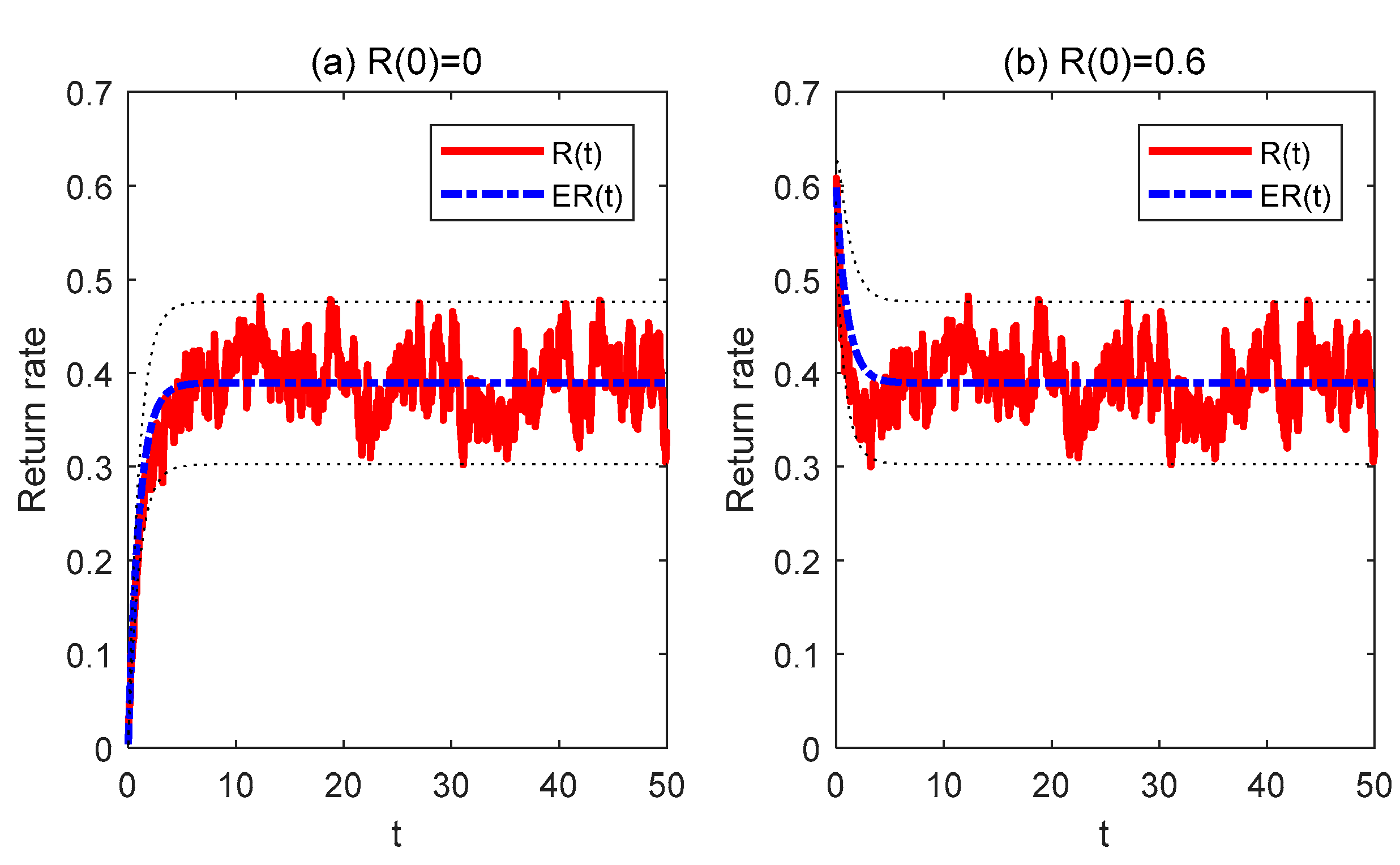
Figure 1 demonstrates how the return rate would tend to be in the presence of stochastic disturbances. Figure 1a shows evolutionary path of the return rate with the initial return rate $R\left(0\right)=0$ and Figure 1b shows the result with $R\left(0\right)=0.6$. The expectation of the return rate will approach the stable state along with the time, whatever the initial return rate. In other words, there exists a unique stable state of the expectation of the return rate for a specific system, and the stable state irrelevant with the initial return rate. The optimal strategy for the third party is to try to keep the system return rate be as close as possible to the stable expectation, even though the initial return rate is higher than the stable state. As a result of the stochastic disturbance, the return rate always hovers around its expectation and could not be possible to approach a stable state. However, the confidence interval of the return rate is stable as the expectation and variance of the return both go for a stable state.

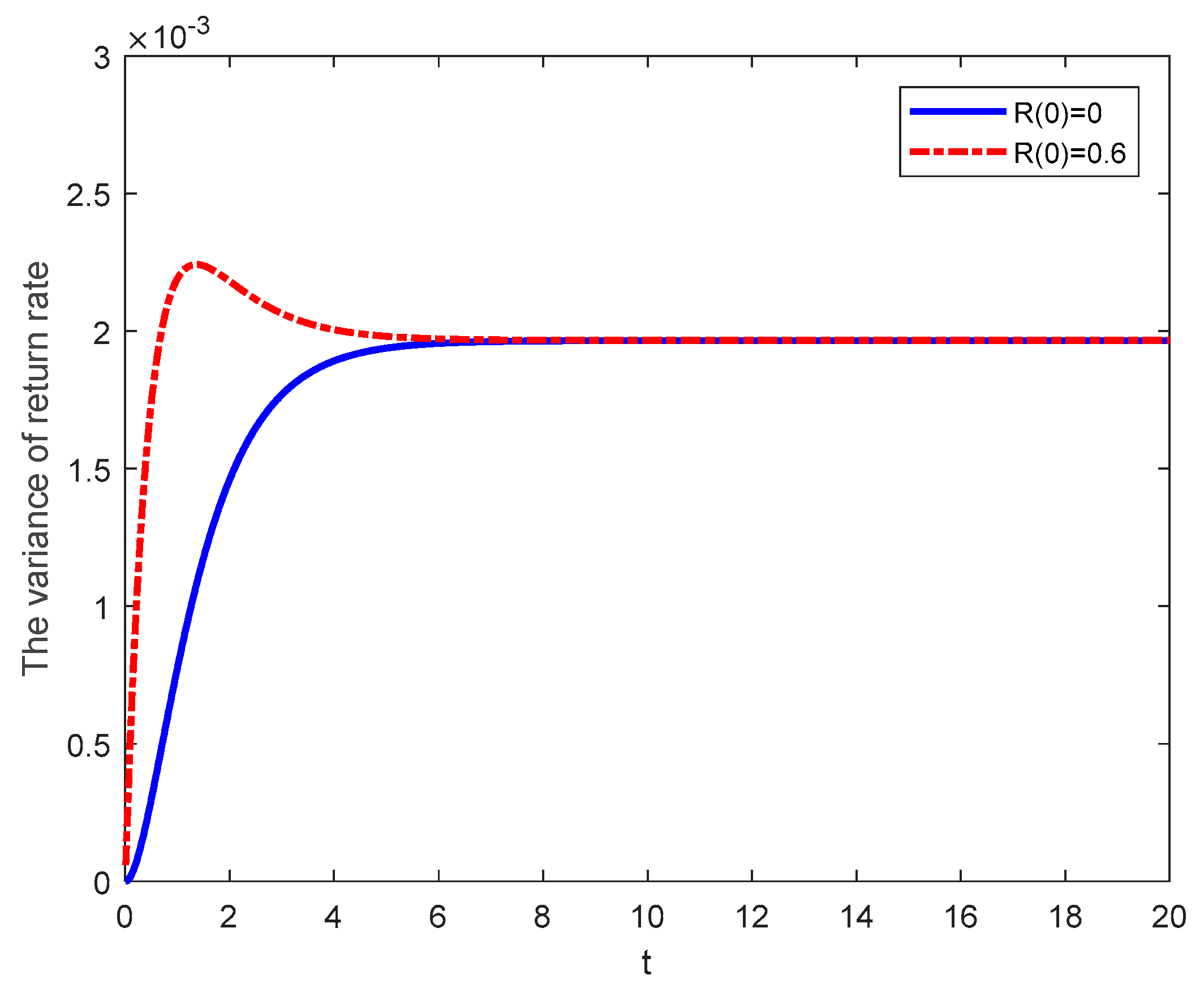
Figure 2 shows how the variance would change along with time. It is evident that there exists a stable state for the variance of the return rate and also the stable state would not be affected by the initial return rate. When the initial return rate is low, the variance will increase with time as the collecting effort grows with time. When the initial return rate is high, the variance would increase very fast and then decrease to approach its stable state. To keep the expectation of the return rate’s smoothly decreasing direction with the stable state, the third party needs to invest higher collecting efforts as the initial return rate is higher under this circumstance. However, the variance of the return rate will approach very close to the stable state after some steps, whatever the initial return rate.

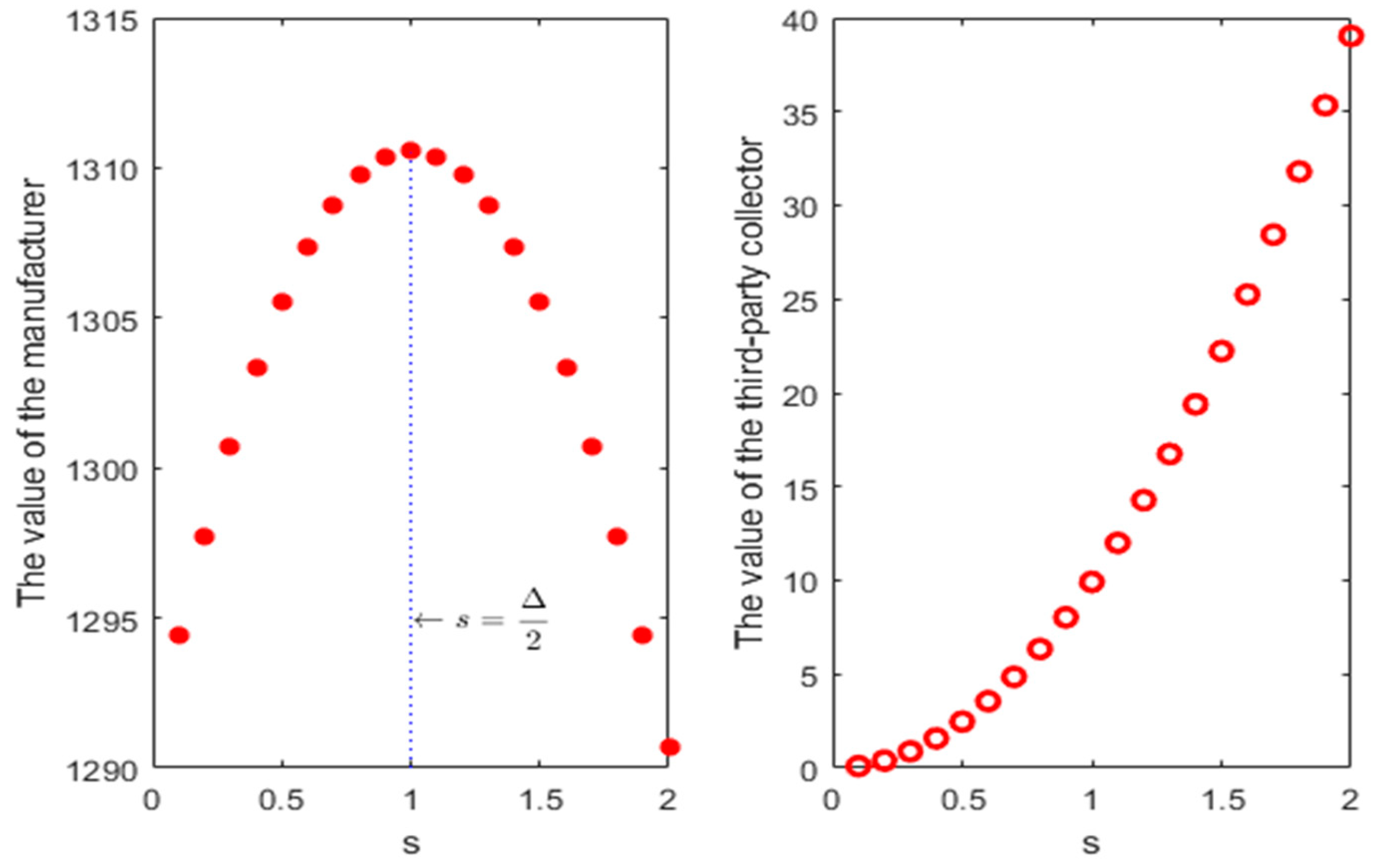
Figure 3 illustrates the impact of the transfer subsidy the manufacturer pays the third party for collecting used products on the profitability of the supply chain members. The profit of the manufacturer increases first and then decreases along with the increasing of transfer subsidy, while the profit of the third-party increases all the time. That is to say, increasing the transfer subsidy would help to give more incentive to the third party on collecting used products. However, the manufacturer would not benefit from the increase of transfer subsidy once the transfer subsidy exceeds a critical value. Given all the unit cost savings from the remanufacturing, this is not the optimal transfer subsidy strategy but given half of the unit cost savings to the third party, it is the optimal transfer subsidy for the manufacturer, i.e., $s^{*}=\mathsf{\Delta }/2$. This result coincides with the result which inferred from the static setting [11]. However, as the value of the third-party is quite small compared to that of the manufacturer, which may cause unfairness feeling for the third party, we argue that the manufacturer should transfer all the unit cost savings to the third party to motivate the third party to collect used products. Although the manufacturer transfers all the unit cost-savings to the third-party, the manufacturer can still benefit from the remanufacturing as the higher transfer subsidy brings higher return rate and thus lower retailer price and higher demand rate for the closed-loop supply chain system.

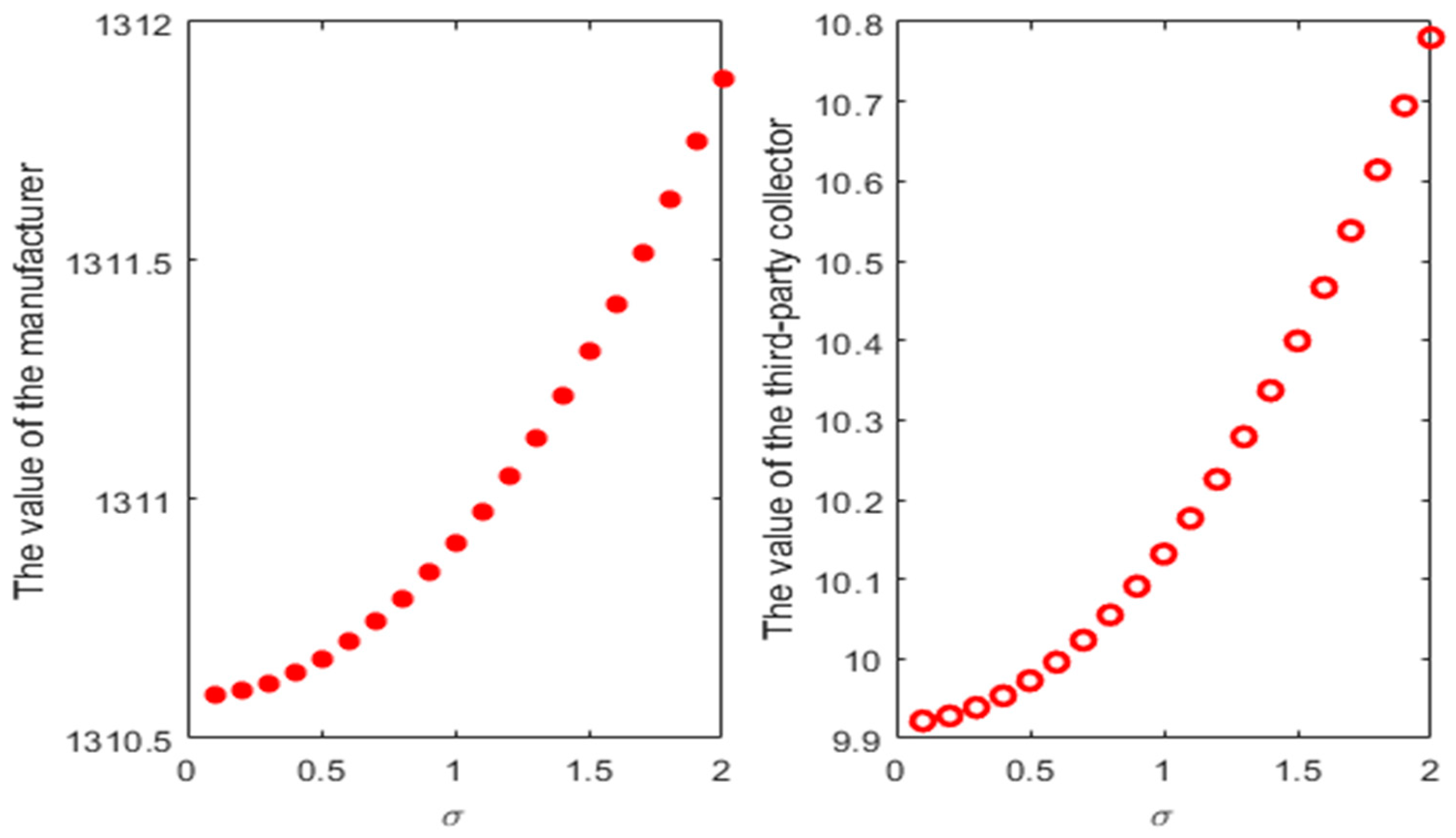
Figure 4 investigates the impact of disturbance intensity on the profitability of supply chain members. As the profit of the retailer and the manufacturer is in the same direction, we can conclude that all the supply chain members can benefit from the increasing of disturbance intensity. This may come from when the disturbance intensity increases, as the third party has to invest more collecting efforts to keep the return dynamics close to the stable state, which results in a higher return rate for the system and thus higher profit for both the manufacturer and the third party. However, the profit increment from the increasing of disturbance intensity is not that remarkable.

5. Stochastic Differential Game with Fairness Concern Followers

In this section, we will extend our model into the scenario of the supply chain with fairness concerns from followers, i.e., the retailer and the third-party collector. To simplify the model, we set the fairness concern coefficients for the retailer and the third party to be same as $\lambda$. We resolve the feedback equilibrium with fairness concern followers in 5.1, the evolutionary path in 5.2, and analyze the impact of fairness concern on the system in 5.3.

5.1. Feedback Stackelberg Equilibrium with Fairness Concern

Denote ${\pi }_{3p}\left(i=m,r,3p\right)$ as the instant profit rate for player $i$ at time $t$, which are given as

$$\begin{gathered} {\pi }_m\left(t\right)=\left(\omega \left(t\right)-c+\mathsf{\Delta }R\left(t\right)\right)D\left(t\right)-sR\left(t\right)D\left(t\right), \\ {\pi }_r\left(t\right)=\left(p\left(t\right)-\omega \left(t\right)\right)D\left(t\right), \\ {\pi }_{3p}\left(t\right)=sR\left(t\right)D\left(t\right)-\frac{1}{2}k{E}^2\left(t\right). \end{gathered}$$

Considering the fairness concern of the followers in the Stackelberg game, the objective functions of the supply chain members are then formulated as

$$\begin{array}{c}\underset{\omega \left(t\right)\ge 0}{\max }\left\{J_m^F=\mathrm{E}{{\displaystyle \int }}_0^{\infty }{e}^{-\rho t}{\pi }_{m}dt\right\},\end{array}$$

(22)

$$\begin{array}{c}\underset{p\left(t\right)\ge 0}{\max }\left\{J_r^F=\mathrm{E}{{\displaystyle \int }}_0^{\infty }{e}^{-\rho t}\left[{\pi }_r-\lambda \left({\pi }_m-{\pi }_r\right)\right]dt\right\},\end{array}$$

(23)

$$\begin{array}{c}\underset{E\left(t\right)\ge 0}{\max }\left\{J_{3p}^F=\mathrm{E}{{\displaystyle \int }}_0^{\infty }{e}^{-\rho t}\left[{\pi }_{3p}-\lambda \left({\pi }_m-{\pi }_{3p}\right)\right]dt\right\},\end{array}$$

(24)

in which $\lambda$ is the fairness concern coefficient for the retailer and the third party. A larger $\lambda$ represents a greater extent of fairness concern for the decision members [31]. The superscript $F$ is used to represent the scenario with fairness followers, and the return dynamics of the objective functions subject to is the same with no fairness scenario, i.e., Equation (1). The followers with fairness concern are trying to maximize their utilities regarding their fairness concern. We also utilize the HJB method to derive the optimal feedback control strategies for the supply chain members. Due to the similarity of the resolution procedure, we omit the details of the resolving of the stochastic differential game with fairness concern followers.

Proposition 4.

When${\theta }_k< \raisebox{1ex}{$\delta \left(\rho +\delta \right)\left(\lambda +1\right)$}\!\left/ \!\raisebox{-1ex}{$b\left(s-{\lambda }_1\right){\mathsf{\Delta }}_s$}\right.$, there exists only one feedback Stackelberg Markov equilibrium in the fairness scenario. The equilibrium control strategies are thus given by

$$\begin{gathered} {\omega }^{F*}\left(R\right)=\frac{a\left(\lambda +1\right)+b\left(3\lambda +1\right)\left(c-\left(\mathsf{\Delta }-s\right)R\right)}{2b\left(2\lambda +1\right)}, \\ {p}^{F*}\left(R\right)=\frac{3a+b\left(c-\left(\mathsf{\Delta }-s\right)R\right)}{4b}, \\ {E}^{F*}\left(R\right)=\frac{\theta }{k\left(\lambda +1\right)}\left(2l_{2}R+l_1\right), \end{gathered}$$

where

$$\begin{gathered} l_1=\frac{\left(s-{\lambda }_2\right)A+4{\sigma }^2{l}_2}{4\left[\rho +\delta -\raisebox{1ex}{$4{\theta }_k{l}_2$}\!\left/ \!\raisebox{-1ex}{$\left(\lambda +1\right)$}\right.\right]}, l_2=\frac{\rho +2\delta -\sqrt{{\left(\rho +2\delta \right)}^2-\raisebox{1ex}{$4{\theta }_{k}b{\mathsf{\Delta }}_s\left(s-{\lambda }_1\right)$}\!\left/ \!\raisebox{-1ex}{$\left(\lambda +1\right)$}\right.}}{\raisebox{1ex}{$8{\theta }_k$}\!\left/ \!\raisebox{-1ex}{$\left(\lambda +1\right)$}\right.}, \\ {\lambda }_1=\frac{\lambda \left(\mathsf{\Delta }\lambda +\mathsf{\Delta }-5\lambda s-3s\right)}{2\left(2\lambda +1\right)}, {\lambda }_2=\frac{\lambda \left(\mathsf{\Delta }\lambda +\mathsf{\Delta }-2\lambda s-2s\right)}{\left(2\lambda +1\right)}. \end{gathered}$$

Proposition 4 shows the feedback control strategies in the fairness concern scenario. It states that the equilibrium price control strategy is the same as that in the setting with no fairness concern. The fairness concern would change the control strategies for the manufacturer and the third-party, and wholesale control price will be lower compared to the scenario with no fairness concern, which means the manufacturer would like to shift some of its profit to the retailer when the retailer is considered to have fairness concerns. However, as the constant setting of the transfer subsidy for the returned used products, the manufacturer cannot shift profit to the third-party. As a result, the incentive of the third party would be lower in the presence of fairness concerns of the third party.

5.2. The Evolutionary Path of the Return Rate with Fairness Concern

Proposition 5 characterizes the evolutionary path of the return rate in the supply chain with fairness concerns from followers. It is obvious that the fairness concern extent would affect the control strategy of the third party and thus the evolutionary path for the return rate.

Proposition 5.

With fairness concern followers, the expectation and variance of the stochastic return rate are given by

$$\begin{gathered} E\left[R^F\left(t\right)\right]=\frac{2{\theta }_k{l}_1}{\varsigma \left(\lambda +1\right)}+\left(R\left(0\right)-\frac{2{\theta }_k{l}_1}{\varsigma \left(\lambda +1\right)}\right)e^{-\varsigma t}, \\ D\left[R^F\left(t\right)\right]=\frac{{\theta }_k{l}_1{\sigma }^2}{{\varsigma }^2\left(\lambda +1\right)}+\frac{\left(R\left(0\right)\left(\lambda +1\right)\varsigma -2{\theta }_k{l}_1\right){\sigma }^2}{{\varsigma }^2\left(\lambda +1\right)}{e}^{-\varsigma t}-\frac{\left(R\left(0\right)\varsigma \left(\lambda +1\right)-{\theta }_k{l}_1\right){\sigma }^2}{{\varsigma }^2\left(\lambda +1\right)}{e}^{-2\varsigma t}. \end{gathered}$$

The long-run stable expectation and variance values of the return rate are calculated by

$$\underset{t\to \infty }{\lim }E\left[R^F\left(t\right)\right]=\frac{2{\theta }_k{l}_1}{\varsigma \left(\lambda +1\right)},\underset{t\to \infty }{\lim }D\left[R^F\left(t\right)\right]=\frac{{\theta }_k{l}_1{\sigma }^2}{{\varsigma }^2\left(\lambda +1\right)}.$$

5.3. The Impact of Fairness Concern on the System

In this subsection, we will further investigate how the fairness concern extent would affect the system dynamics as well as the profitability for the supply chain members by using the numerical method. Figure 5 shows how the fairness concern would affect the dynamics of the stochastic return rate, and Figure 6, Figure 7 and Figure 8 demonstrate the impact of fairness concern on the profitability for the supply chain members. It should be noticed that we utilize the long-run expected profit rate, which gives the instant profit earned from a stable expected perspective, to represent the profitability of the supply chain members.

It is evident that the system with a higher fairness concern extent would result in a lower expected return rate, which means the fairness concern would decrease the enthusiasm for the third-party to collect used-products. As the expected return rate decreases with the fairness concern extent, we could conclude that the collecting efforts will also be reduced with the fairness concern extent. Therefore, the manufacturer needs to give more incentive to the third party in the presence of fairness concerns.

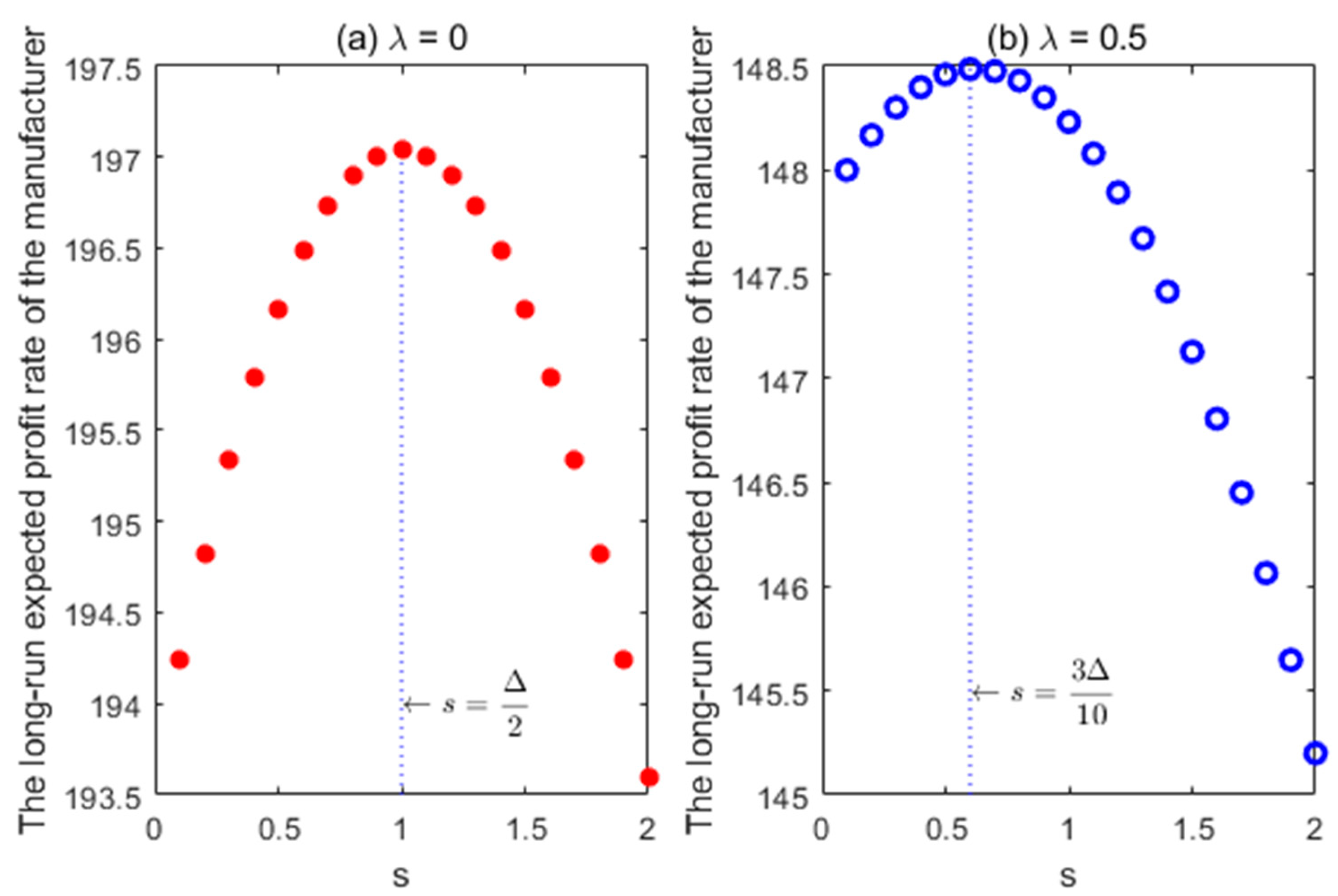
Figure 6 illustrates the optimal transfer subsidy for the manufacturer should be lower in the presence of fairness concern of the third party. The reason for this is the third party collects less when considering the unfairness. As a result, the manufacturer should reduce its optimal subsidy. However, the lower subsidy would result in a lower return rate for the system and lower profit rate for the third party, and thus causing more unfairness for the third-party. When the manufacturer takes the fairness concern into consideration, he will shift some of his profit to other supply chain members. We could conclude from Figure 7 and Figure 8 that the manufacturer only shifts profit to the retailer, while no profit is shifted to the third party. Thus, we argue that the manufacturer should not lower its transfer subsidy; on the contrary, the manufacturer should set a higher subsidy to shift profit and give incentive to the third party.

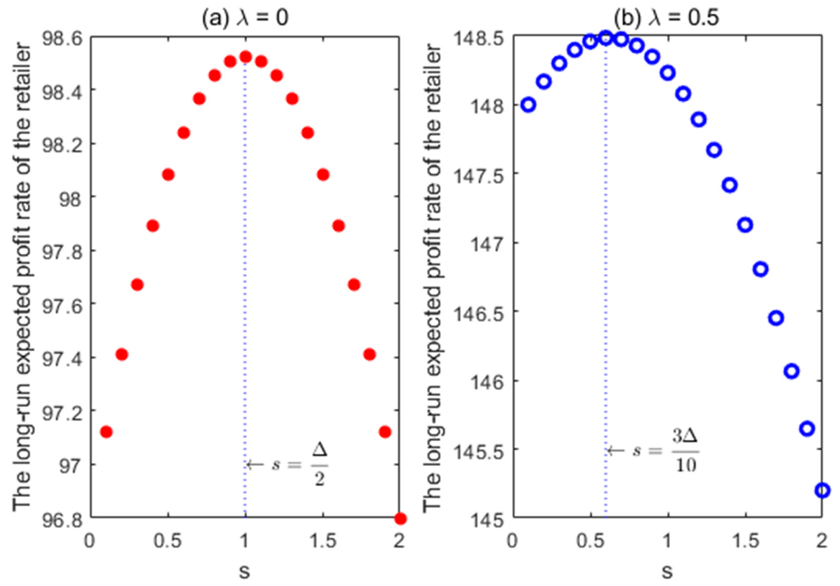
Figure 7 shows that the retailer would make more profit when the manufacturer considers the fairness concerns. As the retail price is unchanged, we could conclude that the extra profit earned by the retailer is shifted from the manufacturer, and the impact of the transfer subsidy on the profitability for the retailer is the same as the manufacturer. When the fairness concern coefficient equals 0.5, the retailer can make a profit rate as much as the manufacturer makes.

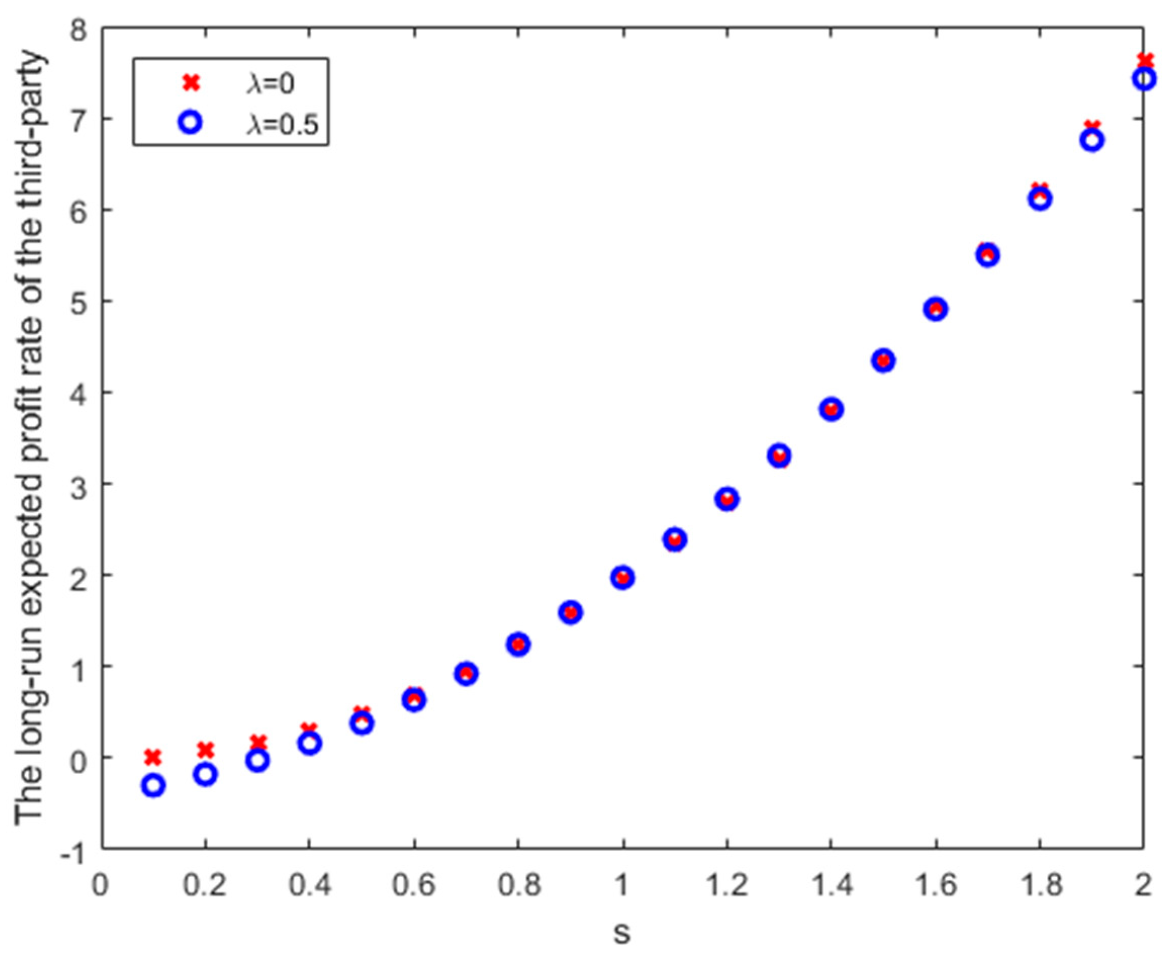
Figure 8 illustrates that the profit the third party earns with and without the fairness concern is quite similar. This mainly comes from the constant setting of the transfer price. The manufacturer could shift profit to the retailer by lower the wholesale price, however, the manufacturer could not do a similar thing to the third party. As the profit rate increases with the transfer subsidy, we argue that the manufacturer should set the transfer subsidy equal to the unit cost savings, to give maximize incentives to the third party for collecting.

6. Conclusions

This paper investigates the dynamic collecting control problem in a closed-loop supply chain consisted of one manufacturer, one retailer, and one third-party collector, in the presence of the stochastic return disturbance. A stochastic differential game model is formulated to discuss the optimal return problem with dynamic characteristics and random factors, and the feedback equilibrium is resolved by the HJB equation method. We also derived the evolutionary path of the stochastic return rate and the value functions of the supply chain members under the optimal control strategies.

We have found there exists only one feedback Stackelberg Markov equilibrium only under a specific condition. The optimal wholesale price and the retail price control strategy decreases with the return rate, and the optimal return control strategy increases with the return rate. As a result of the stochastic disturbance, the evolutionary path cannot be predicted precisely. However, the expectation and variance of the stochastic return rate will both approach a stable state along with the time. We could estimate the interval that the return rate would likely to be with the expectation and variance values. The monotonicity of the expectation and variance is relevant to the initial value of the return rate. However, the expectation and variance both approach the same stable state for a specific closed-loop supply chain system, whatever the initial return rate. The optimal strategy for the third party is to try to keep the system return rate as close as possible to the stable expectation, even though the initial return rate is higher than the stable state. The third party prefers higher transfer subsidy for the used products. However, the manufacturer should not give all the unit cost savings, but rather give half of the unit cost savings to the third party. What is surprising is that all the supply chain members can benefit from the increasing of disturbance intensity.

We further investigate how the presence of fairness concerns would affect the supply chain system. We derived the feedback equilibrium with the retailer and third party as fairness-concerned followers and also the evolutionary path of the stochastic return rate. The results state that third party would lower its collecting effort while the retailer keeps the same retail price regarding the return rate in the context of fairness concern, and the expected return rate will decrease with the extent of fairness concerns. The manufacturer can shift profit to the retailer by lowering the wholesale price, while he cannot shift profit to the third party. As a result, the manufacturer should set the transfer subsidy equals to the unit cost savings of the used product to give incentive to the third party to collect more used products.

This study could be extended in several aspects. Firstly, it would be interesting to investigate how the manufacturer should incentivize the third party to improve the efficiency of the closed-loop supply chain system. Secondly, what would be the optimal strategy when there is more than one member involved in the collecting activities in the supply chain. Also, the optimal return control problem in the supply chain with competing retailers or competing manufacturers is also worthy of further investigation.

References

- Qiang, Q.P. The closed-loop supply chain network with competition and design for remanufactureability. J. Clean. Prod. 2015, 105, 348–356. [Google Scholar] [CrossRef]
- Savaskan, R.C.; Van Wassenhove, L.N. Reverse channel design: The case of competing retailers. Manag. Sci. 2006, 52, 1–14. [Google Scholar] [CrossRef]
- Qiang, Q.; Ke, K.; Anderson, T.; Dong, J. The closed-loop supply chain network with competition, distribution channel investment, and uncertainties. Omega 2013, 41, 186–194. [Google Scholar] [CrossRef]
- Shi, J.; Zhang, G.; Sha, J. Optimal production planning for a multi-product closed loop system with uncertain demand and return. Comput. Oper. Res. 2011, 38, 641–650. [Google Scholar] [CrossRef] [Green Version]
- Giri, B.C.; Sharma, S. Optimal production policy for a closed-loop hybrid system with uncertain demand and return under supply disruption. J. Clean. Prod. 2016, 112, 2015–2028. [Google Scholar] [CrossRef]
- Huang, Z.; Nie, J.; Tsai, S.B. Dynamic collection strategy and coordination of a remanufacturing closed-loop supply chain under uncertainty. Sustainability 2017, 9, 683. [Google Scholar] [CrossRef]
- Ma, Z.; Zhang, N.; Dai, Y.; Hu, S. Managing channel profits of different cooperative models in closed-loop supply chains. Omega 2016, 59, 251–262. [Google Scholar]
- Katok, E.; Pavlov, V. Fairness in supply chain contracts: A laboratory study. J. Oper. Manag. 2013, 31, 129–137. [Google Scholar] [CrossRef]
- Caliskan-Demirag, O.; Chen, Y.F.; Li, J. Channel coordination under fairness concerns and nonlinear demand. Eur. J. Oper. Res. 2010, 207, 1321–1326. [Google Scholar] [CrossRef]
- Nie, T.; Du, S. Dual-fairness supply chain with quantity discount contracts. Eur. J. Oper. Res. 2017, 258, 491–500. [Google Scholar] [CrossRef]
- Savaskan, R.C.; Bhattacharya, S.; Van Wassenhove, L.N. Closed-loop supply chain models with product remanufacturing. Manag. Sci. 2004, 50, 239–252. [Google Scholar] [CrossRef]
- De Giovanni, P.; Reddy, P.V.; Zaccour, G. Incentive strategies for an optimal recovery program in a closed-loop supply chain. Eur. J. Oper. Res. 2016, 249, 605–617. [Google Scholar] [CrossRef]
- Feng, J.; Liu, B. Dynamic impact of online word-of-mouth and advertising on supply chain performance. Int. J. Environ. Res. Public Health 2018, 15, 69. [Google Scholar] [CrossRef] [PubMed]
- Fehr, E.; Schmidt, K.M. A theory of fairness, competition, and cooperation. Q. J. Econ. 1999, 114, 817–868. [Google Scholar] [CrossRef]
- Cui, T.H.; Raju, J.S.; Zhang, Z.J. Fairness and channel coordination. Manag. Sci. 2007, 53, 1303–1314. [Google Scholar]
- Atasu, A.; Sarvary, M.; Van Wassenhove, L.N. Remanufacturing as a marketing strategy. Manag. Sci. 2008, 54, 1731–1746. [Google Scholar] [CrossRef]
- Govindan, K.; Soleimani, H.; Kannan, D. Reverse logistics and closed-loop supply chain: A comprehensive review to explore the future. Eur. J. Oper. Res. 2015, 240, 603–626. [Google Scholar] [CrossRef] [Green Version]
- Govindan, K.; Soleimani, H. A review of reverse logistics and closed-loop supply chains: A Journal of Cleaner Production focus. J. Clean. Prod. 2017, 142, 371–384. [Google Scholar] [CrossRef]
- Huang, M.; Song, M.; Lee, L.H.; Ching, W.K. Analysis for strategy of closed-loop supply chain with dual recycling channel. Int. J. Prod. Econ. 2013, 144, 510–520. [Google Scholar] [CrossRef]
- De Giovanni, P.; Zaccour, G. A two-period game of a closed-loop supply chain. Eur. J. Oper. Res. 2014, 232, 22–40. [Google Scholar] [CrossRef]
- Subramanian, R.; Gupta, S.; Talbot, B. Product design and supply chain coordination under extended producer responsibility. Prod. Oper. Manag. 2009, 18, 259–277. [Google Scholar] [CrossRef]
- Jacobs, B.W.; Subramanian, R. Sharing responsibility for product recovery across the supply chain. Prod. Oper. Manag. 2012, 21, 85–100. [Google Scholar] [CrossRef]
- Jena, S.K.; Sarmah, S.P. Price competition and co-operation in a duopoly closed-loop supply chain. Int. J. Prod. Econ. 2014, 156, 346–360. [Google Scholar] [CrossRef]
- Guide, V.D., Jr.; Van Wassenhove, L.N. Managing product returns for remanufacturing. Prod. Oper. Manag. 2001, 10, 142–155. [Google Scholar] [CrossRef]
- Nakashima, K.; Arimitsu, H.; Nose, T.; Kuriyama, S. Optimal control of a remanufacturing system. Int. J. Prod. Res. 2004, 42, 3619–3625. [Google Scholar] [CrossRef] [Green Version]
- Fallah, H.; Eskandari, H.; Pishvaee, M.S. Competitive closed-loop supply chain network design under uncertainty. J. Manuf. Syst. 2015, 37, 649–661. [Google Scholar] [CrossRef]
- De Giovanni, P.; Zaccour, G. Cost–Revenue Sharing in a Closed-Loop Supply Chain. In Advances in Dynamic Games; Birkhäser: Boston, MA, USA, 2013; pp. 395–421. [Google Scholar]
- Du, S.; Nie, T.; Chu, C.; Yu, Y. Newsvendor model for a dyadic supply chain with Nash bargaining fairness concerns. Int. J. Prod. Res. 2014, 52, 5070–5085. [Google Scholar] [CrossRef]
- Ho, T.H.; Su, X.; Wu, Y. Distributional and peer-induced fairness in supply chain contract design. Prod. Oper. Manag. 2014, 23, 161–175. [Google Scholar] [CrossRef]
- Prasad, A.; Sethi, S.P. Competitive advertising under uncertainty: A stochastic differential game approach. J. Optim. Theory Appl. 2004, 123, 163–185. [Google Scholar] [CrossRef]
- Li, T.; Xie, J.; Zhao, X.; Tang, J. On supplier encroachment with retailer’s fairness concerns. Comput. Ind. Eng. 2016, 98, 499–512. [Google Scholar] [CrossRef]
Figure 1.
The simulation of the stochastic return rate with different initial values. (a) R(0) = 0; (b) R(0) = 0.6.
Figure 2.
The variance of the return rate changes with time.
Figure 3.
The impact of transfer subsidy on the profitability of supply chain members.
Figure 4.
The impact of disturbance variance on the profitability of supply chain members.
Figure 5.
The impact of fairness concern on the return rate.
Figure 6.
The impact of transfer subsidy on the profitability of the manufacturer.
Figure 7.
The impact of transfer subsidy on the profitability of the retailer.
Figure 8.
The impact of transfer subsidy on the profitability of the third party.
© 2019 by the authors. Licensee MDPI, Basel, Switzerland. This article is an open access article distributed under the terms and conditions of the Creative Commons Attribution (CC BY) license (http://creativecommons.org/licenses/by/4.0/).
Share and Cite
MDPI and ACS Style
Xiao, J.; Huang, Z. A Stochastic Differential Game in the Closed-Loop Supply Chain with Third-Party Collecting and Fairness Concerns. Sustainability 2019, 11, 2241. https://0-doi-org.brum.beds.ac.uk/10.3390/su11082241
AMA Style
Xiao J, Huang Z. A Stochastic Differential Game in the Closed-Loop Supply Chain with Third-Party Collecting and Fairness Concerns. Sustainability. 2019; 11(8):2241. https://0-doi-org.brum.beds.ac.uk/10.3390/su11082241
Chicago/Turabian StyleXiao, Jianmin, and Zongsheng Huang. 2019. "A Stochastic Differential Game in the Closed-Loop Supply Chain with Third-Party Collecting and Fairness Concerns" Sustainability 11, no. 8: 2241. https://0-doi-org.brum.beds.ac.uk/10.3390/su11082241
Note that from the first issue of 2016, this journal uses article numbers instead of page numbers. See further details here.