Combined Impact of Socioeconomic Forces and Policy Implications: Spatial-Temporal Dynamics of the Ecosystem Services Value in Yangtze River Delta, China

Abstract

Water can carry or overturn a boat. Natural resources form the foundation of human survival and development. However, land use change caused by human urban civilization has damaged the natural environment and in turn threatened the continuation of human civilization. Accordingly, it is crucial to analyze the impacts of human activities on land use change and consequent dynamics of ecosystem service value (ESV). For the sustainable development of human beings, an investigation should be conducted to explore what type of land use behavior will be considerably beneficial to improve our relationship with the natural environment. This study analyzes the spatial–temporal dynamics of ESV of 148 counties in the Yangtze River Delta in China over three five-year periods (2000–2015) and examines the influence of socioeconomic forces and policy implications. Exploratory spatial data analysis and spatial regression were applied to facilitate the analysis. Results show that the averages of the ESV change ratios of the 148 counties in each of the aforementioned periods are −0.667%, −2.690%, and −4.668%, respectively. The number of counties that showed an ESV loss trend in the three periods are 72 (48.6%), 125 (84.4%), and 139 (93.9%), respectively. In terms of spatial pattern, ESV change demonstrates the spatial distribution characteristic of “high loss spreading from the northeast to the middle and west” with a tendency to strengthen spatial agglomeration. Results of the spatial regression analysis determine the overwhelming importance of population growth and economic advancement. The results also indicate that the development mode characterized by industrial structure, capital input, and technology upgrades can exert considerable influence on socioeconomic development, thereby affecting the change of ESV. Moreover, the constraints of policy substantially affect the changes of ESV from 2010 to 2015. Policy makers should consider the relationship between land use patterns and the ESV variation in different development stages to formulate appropriate measures, thereby reducing or preventing the loss of ecological service value and promoting sustainable development.

1. Introduction

Research on land-use and land-cover (LULC) change over the last decade is one of the core projects in the context of the International Human Dimensions Program (IHDP) and International Geosphere–Biosphere Program (IGBP). Such research clearly demonstrates that human activities result in dramatic changes in landscape pattern and thoroughly affect the climate, biogeochemical cycles, and ecological balance at the global and regional scales. The LULC changes are the most direct and close relationship between humans and the natural world [1,2], in which the former continuously allocate and utilize various land resources to meet humanity’s social and economic development needs [3,4]. Land use patterns include quantity, structure, and spatial pattern [5,6], as well as land use quality, management mode, and productive ability [7,8]. That is, land use changes and transitions comprise a dynamic process that embeds the evolution of landscape structure and land use function. Researches on LULC mapping and change detection has received more attention in recent years. Using accurate remote sensing data and image classification techniques, changes in land use cover and urban environment can be monitored [9,10]. The land use change matrix is widely applied to represent the quantity of land change, while landscape metrics can provide both general and specific information about landscape dynamic patterns [11,12]. The recent development of geographic data analysis methods, including spatial autoregression, neural network [13], spectrum analysis [14], time series analysis [15], cellular automata models [16] and so on, has helped to uncover spatial-temporal dynamics of land use transition and to reach better explanations and predictions of land use evolution.

Natural ecosystem service refers to the vital benefits that humans derive from ecosystems, including food production, nutrient recycling, water regulation, recreation and culture, biodiversity protection, and other supporting services [17,18,19,20,21,22,23]. The majority of the related studies have introduced domain knowledge and auxiliary information for the connotation and techniques of ecosystem service valuation (ESV) [20,24,25,26]. Given the concern for natural resource limitation and constantly emerging environmental problems in recent years, ESV assessment has attracted universal attention in research and policy formulation [17,27,28]. Undoubtedly, LULC change is the most important reason for the variation of ecological service value. ESV is substantially reduced because of the massive transition of cultivated land and woodland and wetland to construction land, while the ecological function of the former land use type is completely lost, thereby leading to far-reaching consequences of environmental problems [29,30,31].

Urbanization is among the most crucial characteristics of human development in the 20th century. Industrialization and urbanization are characterized by population growth, economic agglomeration, and technology advancement, as well as substantially changing the global environment [32,33,34]. China has witnessed an increase in urbanization rates from 19.39% in 1980 to 57.35% in 2016 [35], thereby attracting the world’s attention with its apparent effects on a global scale. Since the implementation of economic reforms and the open-door policy, particularly the opening up and development of Pudong district in Shanghai, the Yangtze River Delta (YRD) has been undergoing thorough and rapid urbanization and industrialization. The YRD range comprises four provincial regions, namely, Shanghai, Zhejiang, Jiangsu, and Anhui. YRD has a clear strategic positioning, including the presence of important international portals in the Asia–Pacific region, world-class metropolitan agglomerations with a globally important modern service industry, and an advanced manufacturing center. The China Urban Agglomeration Development Report (2010) revealed that the YRD urban agglomeration will develop into a world-class city cluster with the strongest comprehensive competitiveness in China in 10–20 years. However, environmental problems, such as the pollution of Tai Lake, security problems of drinking water, loss of high-quality farmland, and air and soil heavy metal pollution are becoming serious [36,37]. Although rapid urbanization promotes rapid social and economic development, this process also weakens the important ecological services provided by the natural ecosystem for cities. The accelerated urbanization and increasingly frequent human activities have exerted large changes in land use and strongly affected ESV [38,39].

Since LULC reflects the most direct and close relationship between human and nature, it is crucial to closely combine it with social, political, and economic issues, especially identifying the impact of enhanced human activities on land use change. In terms of the sustainable development, although human welfare depends on the natural resources provided by the ecosystem, the sustainability, frequency, and density of the impacts of humanity factors on the giant earth system are far more extensive than natural process [40]. Ehrlich and Holden (1971) summarized all humanity factors which can affect the environment as population, product affluence, and technology level and proposed the IPAT equation [41]. In recent years, numerous studies have been conducted to explore the driving forces of land use evolution and have determined the strong effects of population growth, economic conditions, technical level, policy measure, and culture [42,43,44,45]. However, there remains room for improvement to comprehensively analyze the influence of these driving forces and identify the main driving factors in different stages. Furthermore, to support the aim of utilizing natural resources without destroying the resource base, the impact of land use change on the environment and its frequent interaction with human decision-making should be comprehensively understood [46,47]. Thus, enhancing the value of ecological services and promoting sustainable development during urbanization are urgently needed, while the relationship between ecosystem service dynamics and anthropogenic activities should be examined. However, the loss of natural resources appears to be the inevitable price of urbanization, while different development modes and investment levels can have varying impact on the ESV changes. In addition, regional development is not a random independent phenomenon or stationary process over space [48,49,50], while the changes between regions will have evident geographical dependence. Previous studies have confirmed that the positive spatial spillover effects of industry development play an important role in improving urbanization level [51,52], while spatial agglomeration will be one of the most significant characteristics in China’s new urbanization development [53]. Accordingly, the spatial pattern of ESV loss may show spatial dependence and spatial heterogeneity. If we can determine how land use patterns affect ESV variation at different development stages, then we may formulate a solution to delay or even prevent the loss of ESV through policy intervention at different urbanization stages. Although numerous studies have analyzed the effects of landscape patterns on ESV [11,18,54,55], only minimal focus has been on the heterogeneous impact and spatiotemporal variation characteristics of land use transitions on ecosystem services, which is key to investigating the relationship between urban growth characteristics and the consequent loss of ESV. To fill in this gap, the present research attempts to explore the relationship between the variations of ESVs and changes of land use pattern from the spatial and temporal perspectives. Moreover, only a few studies have attempted to jointly analyze the control policy in land use and ecosystem security. Policies can directly or indirectly affect ecosystem structure, change landscape patterns, and manage natural resource utilization to affect ecosystem functioning and change ecosystem service supply [56]. Land use conversion is modulated by land governance through land engineering, economic measures, policies, and institutions [57,58]. However, the impact of constraint policies on land use change and ecosystem services should undergo in-depth analysis.

The aim of our study is to recognize the aforementioned research gap and to identify the dynamic patterns of ESV change and the driving forces related to ESV loss in the YRD region. In particular, the aims of this research are as follows: (1) analyze the land use changes and assess the ESV loss in YRD from 2000 to 2015, (2) depict the spatial-temporal dynamic patterns of ESV in different urbanization periods, and (3) understand the complexities of socioeconomic forces and their causal relations with ESV change.

2. Materials and Methods

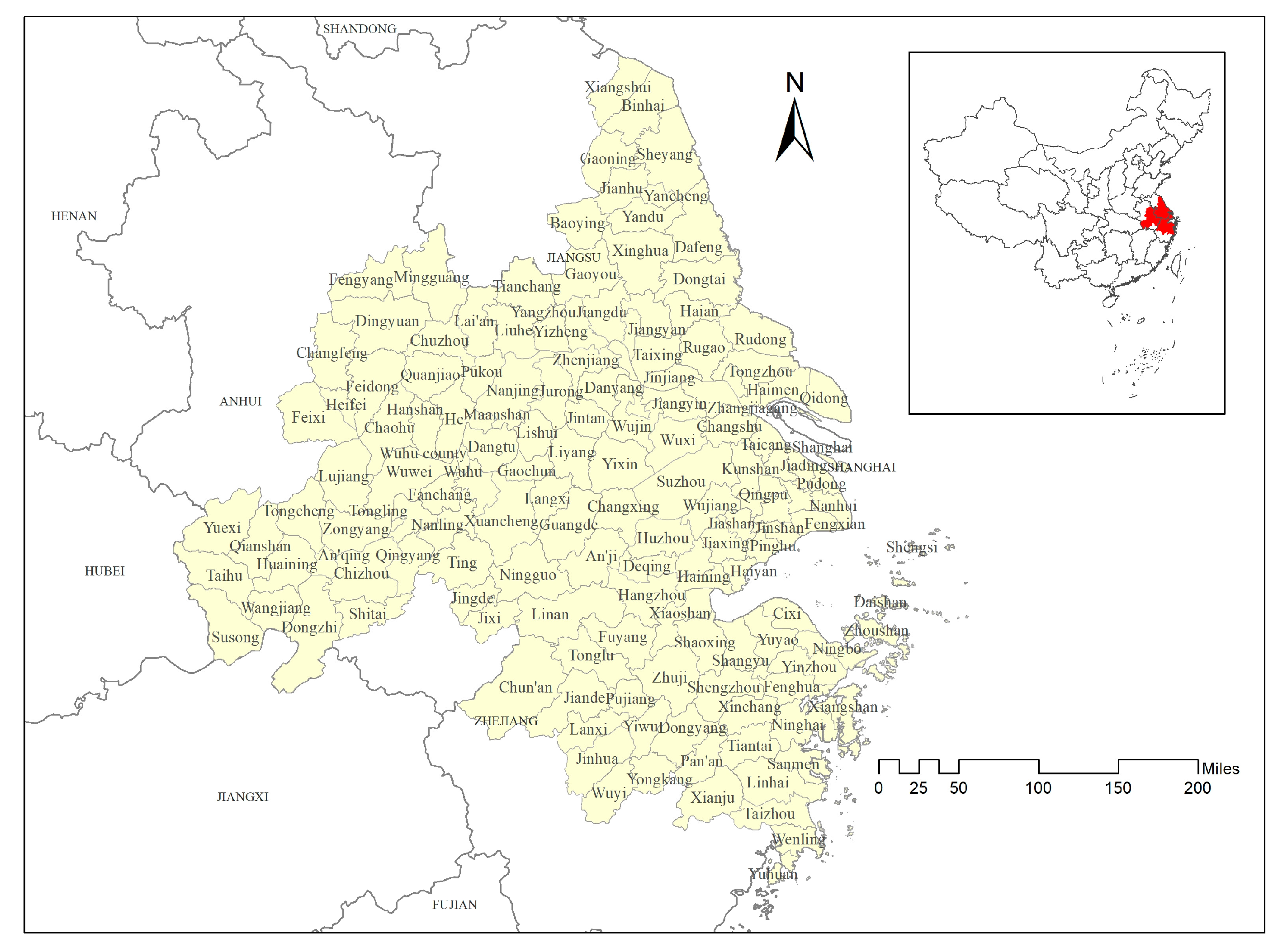
2.1. Study Area

The geographical range of YRD, which is located in an alluvial plain, includes Shanghai Municipality, Zhejiang Province, and Jiangsu Province. This area covers 210,700 square kilometers, which accounts for 2.19% of China’s land area. The YRD region is China’s main economic zone with a population of 156 million and contributes nearly 20% of the gross domestic product (GDP) of the country. As a rapidly developing area of urbanization in China, YRD is a hot spot of substantial land changes and rapid population growth. The current urbanization level is approximately 70%, which is significantly higher than that of the national average. The YRD region remains in the rapid development period and is a substantial attraction to rural–urban immigrants and various industries. This research covers the entire YRD region, which includes one direct-controlled municipality, three subprovincial cities, and 22 prefecture-level cities. The entire area is divided into 148 spatial units consisting of 26 municipal districts and 122 county-level cities (see Figure 1).

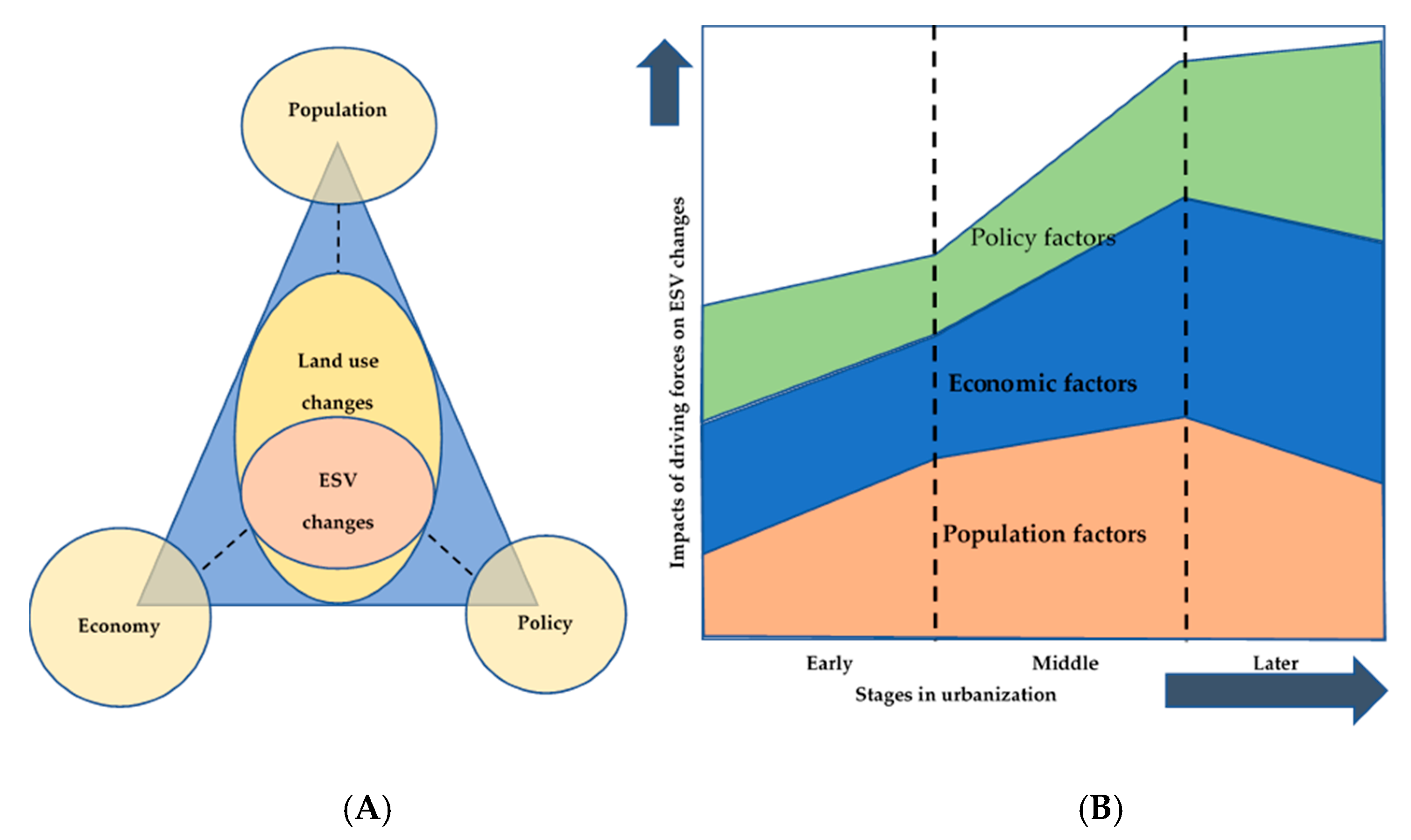
2.2. Analytical Framework

For a limited region, the driving factors of the LULC changes in a certain period are mainly natural factors, socio-economic factors, and land use policy factors [59]. In general, natural factors include environmental change, climate, natural disasters, topography and slope, etc. Given the relatively short research period, changes in natural factors are not significant in our study. In addition, the YRD is a hot spot of rapid population growth and substantial economic advancement, and our literature review enabled us to determine that population, economic, and policy factors are three main driving forces of land use changes and loss of ESV in urbanization. Therefore, we build a theoretical framework containing three aspects: population factors, economic factors, and policy factors (see Figure 2A). In terms of the temporal and spatial ESV dynamics, we suppose that different stages can be influenced by distinct factors and the importance of each factor can vary during these periods (see Figure 2B).

2.3. Data Sources

2.3.1. LULC Data

Accurate land use data are required to precisely assess the ESV change. Accordingly, data on land-use changes from 2000 to 2015 were acquired from the land-use changing investigation developed by the Ministry of Land and Resources (now it has been restructured into Ministry of Natural Resources). The relevant Chinese authorities have consistently updated the land use change database based on the annually conducted surveys and remote sensing monitoring since 1996. Each survey table covers reliable information of land area in various types and years along with the transition among different types. Given that the land-use change investigation adopted different land cover classification criteria in the entire study periods, the current study unified such land use classification standards into seven categories, namely, farmland, forest land, grassland, built-up land, water body, wetland, and unused land. The entire research period was divided into 2000–2005, 2005–2010, and 2010–2015.

2.3.2. Driving Factors Data

Based on the analytical framework, a total of 12 potential factors from the perspectives of population, economy, and policy were chosen referring to the existing literature and available data (see

Table 1. Descriptive statistics of selected explanatory variables.

Category	Dimensions	Factors	Abb	Max	Min	Mean	Std.	Skew	Kurt
Population factors	Population urbanization	Urban permanent residents (104)	UPP	875.0	7.8	91.8	93.0	4.71	27.27
		Population density (person/km2)	PD	7925.0	65.1	802.0	866.0	3.86	20.69
Economic factors	Economic growth	GDP per capita (yuan)	GDPPC	389,873.4	2030.5	42,053.9	43,321.3	2.57	11.00
		Secondary and tertiary industries products (108 yuan)	STIP	9674.7	1.37	469.9	1016.3	5.23	33.39
	Industrial structure	Share of secondary industry in GDP (%)	S_share	85.5	5.8	50.0	0.1	−0.70	0.62
		Share of tertiary industry in GDP (%)	T_share	88.5	2.9	36.5	0.1	1.10	4.04
	Investment	Total investment of fixed asset (108 yuan)	TIFA	4750.8	1.13	263.6	494.1	4.76	30.05
		Foreign direct investment (104 USD)	FDI	1,011,101.0	8.0	30,262.6	80,780.5	6.47	55.80
		Road density (102 m/km2)	RD	350.0	31.7	103.6	51.4	1.40	2.54
Policy factors	Urban planning and land-use policy	1 = optimized development; 0 = no such policy	Pol_1	1	0	0.3	0.5	0.86	−1.28
		1 = core development; 0 = no such policy	Pol_2	1	0	0.3	0.5	0.90	−1.21
		1 = limited development; 0 = no such policy	Pol_3	1	0	0.4	0.5	0.48	−1.80

). Population urbanization is an important force of LULC changes and it can be reflected by total quantity and population density [42,43,44,45]. For economic factors, we set three dimensions to specifically reveal the impact, that is, economic growth, industrial share, and investment were considered to represent quantity growth, structure change, and technical input (associated with the economic quality) [44,60,61]. Although policy factors are difficult to express quantitatively and spatially [62], we attempt to examine the binding effect of urban planning and land use policy.

We collected the socioeconomic data of 148 districts and counties of YRD. The urban permanent residents, population density, GDP per capita, secondary and tertiary industry products, share of the secondary and tertiary industries in GDP, and total investment of fixed asset were collected from the China County Statistical Yearbook (CCSY). The data of foreign direct investment and road density were obtained from the annual county statistical bulletin for each year, while the policy type information was acquired from the YRD urban agglomeration development plan. All data were collected for 2000, 2005, 2010, and 2015 and Table 1 lists the descriptive statistics of explanatory variables. The change amounts of every five years were calculated and all explanatory variables were spatially matched with 148 counties. In addition, we used the variance inflation factor (VIF) to test whether multicollinearity exists among the explanatory variables and the computed results showed that all VIFs of the explanatory variables are below 10, thereby indicating that multicollinearity did not exist among the explanatory variables.

2.4. ESV Assessment

The ESV calculation has become a popular topic in global sustainable development ecological economic and environmental issues [30,31]. Costanza et al. (1997) proposed the basic guidance and valuation methods [20]. In China, Xie et al. (2008) considered the local ecological characteristics, classified the country’s terrestrial ecosystem into six ecosystems, and posed appropriate adjustments to the ecological services value coefficient [24]. A proxy method that matches the land use type to equivalent biomes is widely adopted by Chinese scholars on the basis of the service value table of unit area of China’s terrestrial ecosystem [63,64]. This study adopted this method as well, and by applying the data of grain products of per unit (ha), the standard ecosystem service equivalent value nationwide was revised to that of the research area. Specifically, ecosystem services value equivalent factor is the relative contribution rate of the ecosystem’s potential service value, and its unit value is equal to one-seventh of the value of annual grain product per hectare. The average annual grain yield in the Yangtze River Delta region from 2000 to 2015 was 5638.37 kg/ha, and the average grain price in 2015 was 2.57 RMB/kg. Therefore, the unit value of equivalent factor in the Yangtze River Delta region was 2066.86 RMB/ha/year. Then, we multiplied it with ecosystem services equivalent factor per unit area in China to obtain the revised ESV coefficient (2.335 times of the nationwide level) [65]. Note that our ESV calculation adopted the overall coefficient of each ecosystem biome type instead of the specific coefficients for each ecosystem service. ESV of YRD at four time points (i.e., 2000, 2005, 2010, and 2015) were valuated and the formula was as follows:

$$\mathrm{ESV}={\displaystyle \sum }\left(A_k\ast V{C}_K\right),$$

(1)

wherein, $A_K$ and $V{C}_K$ denote the acreage and value coefficient (the revised ESV coefficient in

Table 2. Ecosystem service value (ESV) coefficient (RMB/ha/year).

LULC Type	Farmland	Forest Land	Grassland	Water Body	Wetland	Unused Land
ESV equivalent factor a	6.91	21.85	7.24	45.97	62.71	0.42
Nationwide ESV coefficient a	6114	19,334	6406	40,676	55,489	371 b
Revised ESV coefficient	14,281	45,158	14,963	95,008	129,606	867

Source: ^a [24,65]; ^b [66].

), respectively, for the ecosystem biome of each land use type “k”.

To compare the intensity of the ESV changes, we further calculated the ESV change ratio in three periods from 2000 to 2015 at the YRD county level. The ESV change ratio is expressed as follows:

$$R_{esv}=\frac{ES{V}_{t_2}-ES{V}_{t_1}}{ES{V}_{t_1}}\ast 100\%,$$

(2)

where t₁ and t₂ are the initial and final years, respectively, of each period and $ES{V}_{t_1}$ and $ES{V}_{t_2}$ are ESVs at times t₁ and t₂, respectively. The ESV change ratio is expressed as R_p1 for period 1 (i.e., 2000–2005), R_p2 for period 2 (i.e., 2005–2010), and R_p3 for period 3 (i.e., 2010–2015). The low change ratio value means high ESV loss, while the change ratio values near or above 0 indicate that ESV has minimal change or even improvement.

2.5. Exploratory Spatial Data Analysis

Our study utilizes exploratory spatial data analysis (ESDA) to measure whether the attributes in neighboring areas are generally similar or dissimilar [67,68]. ESDA is widely used to explore global and local spatial agglomeration or spatial outliers and reveal the spatial interaction between various spatial elements [69].

2.5.1. Global Spatial Autocorrelation

We used global Moran’s I index for global spatial autocorrelation to identify whether spatial significant autocorrelations can be found in the distribution of spatial objects. Moran’s I value is expressed as follows:

$$I=\frac{k{{\displaystyle \sum }}_{i=1}^k{{\displaystyle \sum }}_{j=1}^k{W}_{ij}\left(x_i-\overline{x}\right)\left(x_j-\overline{x}\right)}{{{\displaystyle \sum }}_{i=1}^k{{\displaystyle \sum }}_{j=1}^k{W}_{ij}{{\displaystyle \sum }}_{i=1}^k{\left(x_i-\overline{x}\right)}^2},$$

(3)

where $x_i$ and $x_j$ denote the actual attribute values in regions i and j, respectively; $\overline{x}$ represents the mean value of the observations; $W_{ij}$ is a spatial weight matrix with one to describe the position where i is adjacent to j and zero otherwise; n represents the number of observed spatial units. In order to further test the significance of the spatial autocorrelation, the standardized statistical Z value was calculated and specific operational formula is shown as below:

$$Z_{score}=\frac{I-E\left(I\right)}{\sqrt{VAR\left(I\right)}},$$

(4)

where E(I) is the mean of Moran’s I and $VAR\left(I\right)$ refers to the variance of Moran’s I. A value of Moran’s I approximating 1 or −1 under the circumstance of the significance level p = 0.05 means similar observations show characteristic of spatial agglomeration. If the value of I approximates 0, the distribution of spatial units tends to be random or there is no spatial autocorrelation between the observed sample and its adjacent region.

2.5.2. Local Spatial Autocorrelation

Referring to the related studies by Anselin [70], the local indicator of spatial association (LISA) was put forward to evaluate the clustering in individual spatial units. The LISA model is defined as follows:

$$I_i=\frac{n\left(x_i-\overline{x}\right){{\displaystyle \sum }}_i{w}_{ij}\left(x_j-\overline{x}\right)}{{{\displaystyle \sum }}_i{\left(x_i-\overline{x}\right)}^2}=Z_i{\displaystyle \sum }_j{W}_{ij}{Z}_j,$$

(5)

where $I_i$ represents the indicator of spatial association (i.e., LISA) and $Z_i$ and $Z_j$ are generated through normalizing $x_i$ and $x_j$, respectively. A positive $I_i$ refers to significant local spatial clusters. That is, the local spatial samples with similar attribute values show the tendency of spatial agglomeration, Thus, those observed units will form type either High–High (HH) clusters or Low–Low (LL) clusters in the Moran’s I scatter plot. On the contrary, a negative $I_i$ indicates the similar value of local spatial units shows the dispersion distribution, that is, the observed units with high (low) value are adjacent to other units with low (high) values, thereby forming High–Low (HL) or Low–High (LH) clusters. In the Moran’s I scatter plot, the HH clusters or LL clusters are represented by the first and third quadrant while HL clusters or Low–High (LH) clusters are represented by the second and fourth quadrant.

2.6. Spatial Regression Model

We applied the ESDA method to check whether the spatial pattern of the ESV loss shows spatial autocorrelation or spatial heterogeneity characteristics. Furthermore, we intend to work with the regression relationships involving sample data that are spatial because spatial data typically violate the assumption that each observation is independent of other observations made by ordinary regression methods [71]. Regression relationships involving spatial data are needed to answer the questions of interest in regional science, including spatial dependence and spatial heterogeneity.

Table 3. Description of three regression models.

Model Type	Specified Formulation	Parameter Description
Standard Linear Regression	$\mathrm{Y}=\mathrm{X}\beta +\epsilon$	Y: (n × 1) vector of response variables X: (n × k) matrix of explanatory variables $\beta$: regression coefficient W: (n × n) spatial weight matrix $\mathsf{\rho }$: spatial lag parameter to be estimated $\mathsf{\mu }$: error term $\epsilon :\left(\mathrm{n}\times 1\right)$ vector of independent (indeterminate) error terms
Spatial Lag Model	$\mathrm{Y}=\mathrm{X}\mathsf{\beta }+\mathsf{\rho }\mathrm{WY}+\mathsf{\epsilon }$   ε~N (0, δ2)
Spatial Error Model	$$\begin{gathered} \mathrm{Y}=\mathrm{X}\mathsf{\beta }+\mathsf{\mu } \\ \mathsf{\mu }=\mathsf{\rho }\mathrm{W}\mathsf{\mu }+\mathsf{\epsilon } \end{gathered}$$    ε~N (0, δ2)

presents the formulation and characteristics of standard linear and spatial regressions, including spatial lag and error models. In a standard linear regression model, the error terms are independently and randomly subjected to the normal distribution [72,73]. If a spatial dependence exists in the errors, then standard linear regression cannot meet the demand to yield valid results [74]. The spatial autoregressive model is an appropriate methodology for identifying the spatial variation and reflecting the local spillover effects. For the spatial lag models (SLM), spatial autocorrelation is defined by a linear relation between the response variable (y) and associated spatially lagged term (WY); for spatial error models (SEM), spatial autocorrelation is described by an error term (u) and associated spatially lagged error term ($\mathrm{W}\mathsf{\mu }$) [75].

3. Results

3.1. Change of ESV

The change ratio of ESV is an effective measure to investigate the general trend and intensity of the ESV change of each county. Therefore, we calculated the ESV change ratio for 148 counties in YRD through three periods from 2000 to 2015 (see Figure 3). The results show that from 2005 to 2015, an increasing number of counties faced the reduction of ESV, while only a few counties manifested an increase in ESV. Accordingly, ESV loss is an inevitable trend in the urbanization process.

Table 4. Description index of the ecosystem services value change ratio (%).

Study Period	Max	Min	Mean	Std.	Median
Period 1	18.894	−16.518	−0.667	5.672	0.068
Period 2	17.775	−24.966	−2.690	6.590	−1.876
Period 3	11.807	−17.238	−4.668	6.486	−1.894

provides the description index of the ESV change ratio. The mean of change ratio in period 1 (2000–2005), period 2 (2005–2010), and period 3 (2010–2015) are −0.667%, −2.690%, and −4.668%, respectively. In addition, the maximum value of ESV change ratio was evidently decreased, while the minimum value decreased first and increased thereafter.

To better understand the spatial visualization process of the ESV change patterns, this research divided the ESV change ratio of each county in the study area to five classes (every five percentage points). Figure 4A–C show the spatial and temporal disparities of the ESV change ratio for the three periods. The majority of the areas show an ESV loss tendency throughout the study period.

A total of 72 (48.6%), 125 (84.4%), and 139 (93.9%) counties showed ESV loss trend in the aforementioned three periods, respectively. In terms of the severity of ESV loss, the counties with ESV loss between 0% and 5% in the first period comprised 35.8% of the total, which added to 56.0% in the second period, and gradually increased to 66.8% in the third period. This result is mainly caused by several counties that showed an increase trend in the first period but decreased in the second period. In addition, the counties that showed a 5%–10% ESV loss in each of the three periods accounted for 4.7%, 20.3%, and 12.8%, thereby revealing a trend of initially increasing and decreasing thereafter. For the counties with a change rate above 10%, the number reached 8.8% and 14.8% in the first and third periods, respectively, thereby indicating that numerous counties have experienced substantial reductions in ESV.

Furthermore, the spatial disparities in the ESV change ratio from 2005 to 2015 showed the spatial distribution pattern of “high loss spreading from the northeast to the middle and west.” Thus, high-loss areas were first distributed in the northeast of YRD, including northern Jiangsu (e.g., Xiangshui, Sheyang, Dafeng, and Dongtai) and eastern Shanghai (e.g., Jiading, Nanhui, and Fengxian). The middle and western areas eventually turned to high-loss areas. These areas are in western Jiangsu (e.g., Danyang, Wujin, and Gaochun) and eastern Anhui (e.g., Maanshan, Dangtu, Fanchang, and Wuhu).

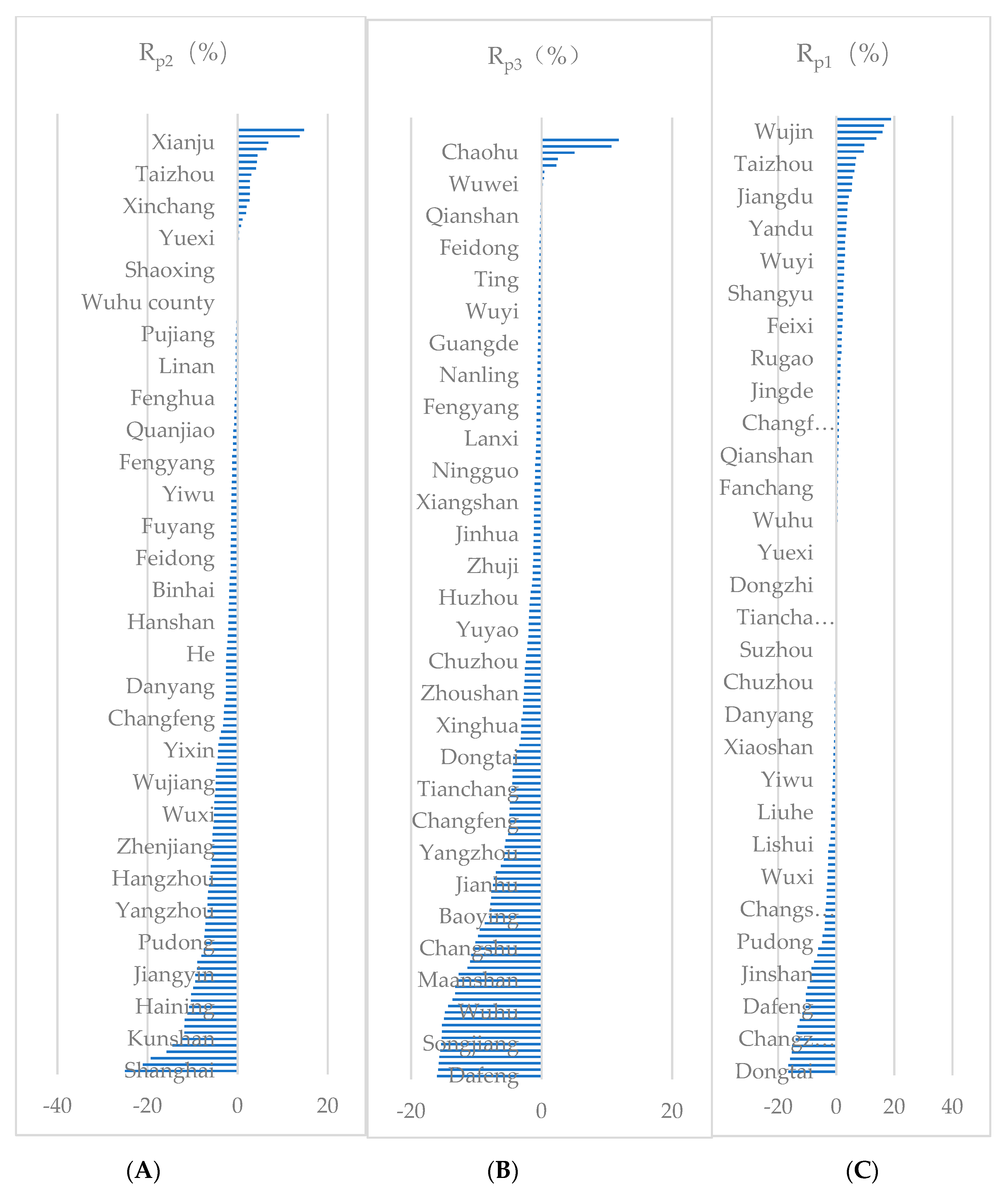
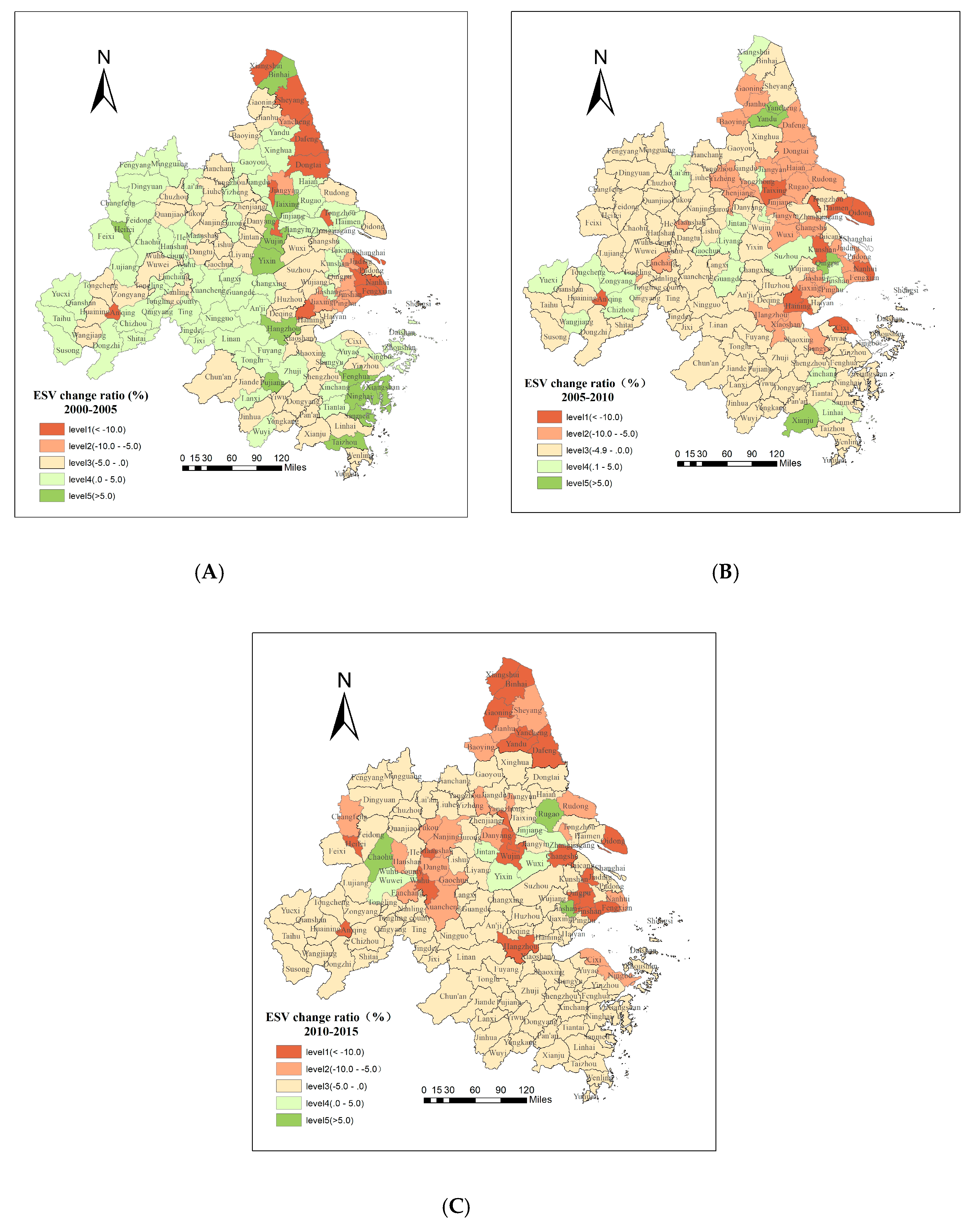
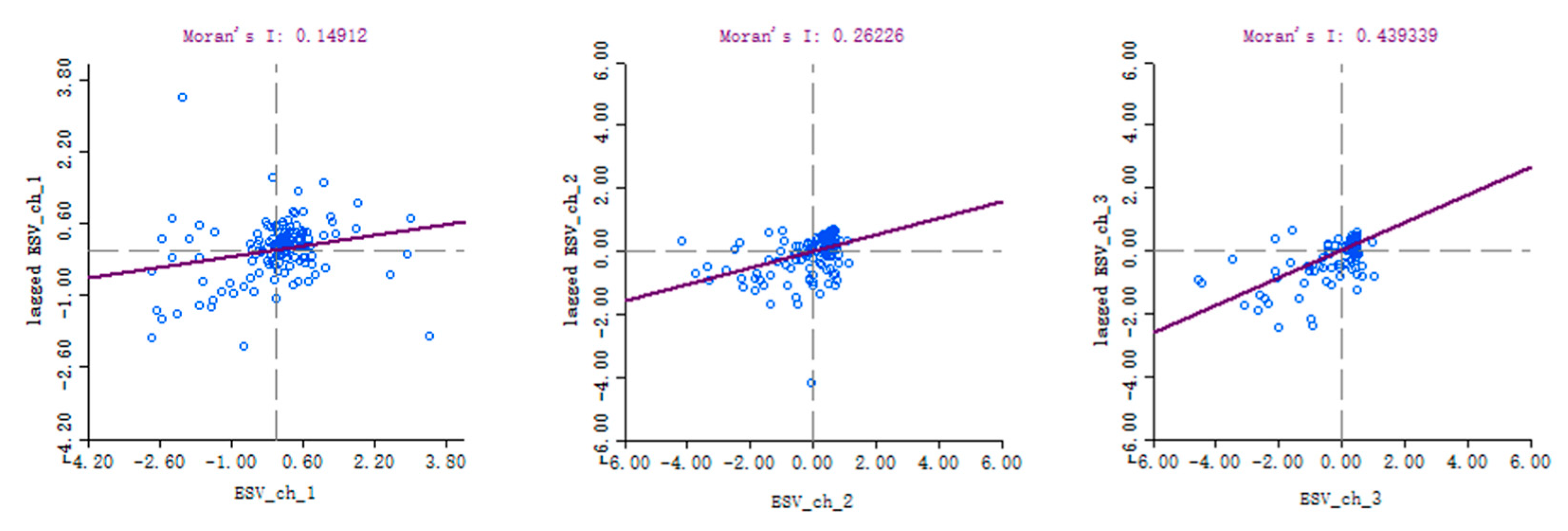
3.2. Spatial Pattern of Changes of ESV

Numerous studies have supported that the regional socioeconomic development is not a closed system [48,50]. Thus, the loss of ESV can be affected by its factors and external situations in its surrounding area [69].

Figure 5 shows the Moran Scatter plot of the ecosystem value change of the 148 counties in YRD from 2000 to 2015. The results demonstrate that the global Moran’s I values of the ESV change were 0.1491, 0.2622, and 0.4393 for in periods 1 (2000–2005), 2 (2005–2010), and 3 (2010–2015), respectively. Given that the global Moran’s I values in the 148 spatial units in the study area were above 0 and the standardized statistic Z value is positive under significance level p = 0.05, the null hypothesis that there exists no spatial correlation of ESV change across the counties can be rejected. The positive Moran’s I value in the three periods indicates that the spatial agglomeration occurs in regions where the extent of ESV change show similarity in the area. The spatial agglomeration of ESV change increased throughout the study period, thereby demonstrating that the degree of spatial agglomeration tends to strengthen in the entire study period.

The LISA value of the three study periods are calculated to acquire an improved understanding of the internal conditions to further examine the contribution of each spatial unit to the global agglomeration. The results can be applied to identify the hot-spot and cold-spot areas to provide an improved explanation of the spatial heterogeneity characteristics of the ESV loss for each spatial unit. The LISA cluster map presented the significant regions with spatial heterogeneity characteristics (see Figure 6).

The results show that the ESV loss of each region in YRD shows an apparent characteristic of spatial agglomeration. The type of LL regions are the agglomeration areas with low ESV loss. In period 1, under the condition of significance level p = 0.05, the cold-spot regions of type LL were relatively dispersed. These counties include Feixi, Changxing, Ting, Jiande, and the middle area of Zhejiang Province, such as Xinchang, Ninghai, Tiantai, and Panan. Thereafter, the distribution pattern of type LL regions demonstrated a clear dynamic process of centralization toward the west (especially in period 2), with its number and scale expanding gradually. Counties, including Yuexi, Taihu, Susong, Chaohu, and Chizhou, were added to this region. Until period 3, the western area of Zhejiang Province, including Chunan and Jiande, have been added to this type.

Compared with the Type LL regions, Type HH counties represent hot-spot regions with the clustering of spatial units of high ESV loss. Figure 6A–C show an apparent increase in the Type HH areas. In the beginning of the study periods, two distinct regions of Type HH existed. One was located north of Jiangsu Province, including Yancheng, Yandu, and Dafeng. The other evident Type HH region included Jiading, Pudong, Nanhui, Fengxian, Jiashan, Jiaxing, and Haiyan, which are located in Shanghai and northern Zhejiang Province. Through period 2, the Type HH regions expanded along the Yangtze River and Hangzhou Bay. Counties, including Nanjing, Zhenjiang, Yizheng, Jinjiang, Ningbo, Cixi, Yuyao, and Xiaoshan, have been added to this type of region. When the LISA cluster map of periods 1 and 3 were compared in 2000–2005, no Type HH counties in the west or south of the study area can be observed. In 2010–2015, the situation was relatively different because these counties, including Changfeng, Hefei, Feixi, Linhai, Taizhou, and Wenling, proved the gradual extension of the Type HH counties to the west and south of YRD.

In addition, Types LH and HL regions represent the agglomeration of dissimilar values, thereby showing negative local spatial autocorrelation. Neither Type LH or Type HL showed in period 1. Type LH counties did not show centralized distribution until period 3 and these counties mainly included Kunshan, Pinghu, Jiading, and Pudong, which are adjacent to Type HH counties in Shanghai. For Type HL counties, only Hefei and Changsu in periods 2 and 3, respectively, were included in this agglomeration type.

3.3. Spatial Regression Model Estimation

To examine the impact of various factors and the importance of each factor during different periods, the study selected 12 independent variables for the regression analysis. Before conducting the spatial regression, we performed a series of diagnostic tests to confirm whether the spatial dependency is embodied by the spatial lag of the response variable or the unknown error term [76]. The Lagrange multiplier (LM) test for spatial lag autocorrelation and error dependence are performed by applying the OLS residuals and spatial weights [75]. The LM lag and LM error tests are significant for the models in periods 1 and 3 (rows 1–2 in

Table 5. Diagnostic results on the nature of spatial dependency (spatial lag or error terms). (dependent variable: ln (ESV loss) in each period; N = 148).

	Period 1	Period 2	Period 3
LM (lag)	8.661 *** (0.0032)	4.682 ** (0.0329)	6.472 ** (0.0108)
LM (error)	8.023 *** (0.0046)	1.726 (0.1923)	4.222 ** (0.0399)
Robust LM (lag)	4.559 *** (0.0035)	/	4.059 *** (0.0069)
Robust LM (error)	2.197 (0.1681)	/	1.809 (0.1786)
Adjusted R2 (OLS)	0.562	0.466	0.503
Adjusted R2 (lag)	0.643	0.625	0.653
Adjusted R2 (error)	0.566	0.592	0.534

Note: *** significance at 1% level; ** significance at 5% level.

). Therefore, we applied the robust Lagrange multiplier (LM) test for spatial lag autocorrelation and error dependence to determine the proper model [76,77]. The robust LM (lag) test was significant, whereas the robust LM (error) was not significant (rows 3–4 in Table 5). For period 2, LM (lag) was significant, while LM (error) was not significant. Thus, SLM is an ideal choice. In summary, we preferred SLM for the regression throughout the study period. As alternative, we conducted an OLS, spatial lag, and spatial error models separately.

Table 6. Estimating results of regression models for ESV loss.

Period 1 (2000–2005)				Period 2 (2005–2010)			Period 3 (2010–2015)
	OLS	SLM	SEM	OLS	SLM	SEM	OLS	SLM	SEM
lnUPP	0.238 ***	0.249 ***	0.250 ***	0.039 **	0.040 **	0.041 **	0.059	0.060	0.062
lnPD	0.109 **	0.083 ***	0.081 **	0.171 ***	0.171 ***	0.174 ***	0.086 *	0.089 *	0.081
lnGDPPC	0.236 **	0.265 **	0.260 ***	0.139 **	0.139 **	0.155 ***	0.153	0.163	0.171
lnSTIP	0.356 ***	0.357 ***	0.358 ***	0.143 **	0.143 **	0.161 ***	0.151	0.145	0.125
S_share	0.255 *	0.211 *	0.172	0.053 **	0.053 **	0.049 **	0.130 **	0.131 **	0.131 **
T_share	0.166 *	0.158 *	0.146	0.108 ***	0.108 ***	0.106 ***	0.298 ***	0.288 ***	0.315 ***
lnTIFA	0.209 ***	0.195 ***	0.207 ***	0.304	0.315	0.312	0.132	0.129	0.130
lnFDI	−0.028	−0.020	−0.016	−0.003	−0.004	0.001	−0.111 ***	−0.111 ***	−0.108 ***
lnRD	0.080 **	0.065 **	0.071 **	0.032	0.045 *	0.038 *	0.158 ***	0.154 ***	0.155 ***
Pol_1							−0.096	−0.122	−0.122
Pol_2							−0.224 ***	−0.238 ***	−0.249 ***
Pol_3							−0.262 ***	−0.269 ***	−0.281 ***
W×lnY		0.296 ***			0.288 ***			0.365 ***
W×μ			0.328 ***			0.303			0.349 **
Constant	0.309 ***	0.465 **	0.274 **	0.785 ***	0.792 **	0.769 ***	−0.397 **	−0.156	−0.392 **
Adjusted R2	0.562	0.643	0.566	0.466	0.625	0.592	0.503	0.653	0.534

Note: *** significance at 1% level; ** significance at 5% level; * significance at 10% level.

lists the results of the parameter estimation of the three regression models in the three periods. In period 1, W × lnY was significantly correlated with the ESV loss in SLM (p < 0.01), while the estimated coefficient reached 0.296 and 0.328 in SLM and SEM, respectively. These results indicated that the response variable ESV loss had strong spatial endogenous correlation effect. That is, if other explanatory variables are controlled, then each 1% increase in ESV loss in the neighboring areas will lead to at least 0.3% increase in the local ESV loss. Similar characteristics can be observed in periods 2 and 3. The SEM model results showed that $\mathrm{W}\times \mathsf{\mu }$ had significant correlation with the response variable in periods 1 (p < 0.01) and 3 (p < 0.05). Hence, the error term also has spatial correlation effect in the regression model, thereby indicating the existence of omissive explanatory variables that show space correlation as well.

Table 6 shows the estimation results of the three types of regression models. Given that SLM has been tested to be the most suitable for the spatial regression in this study, we focused generally on the significance of each explanatory variable in SLM. Population urbanization plays an extremely important role in the ESV change. The variable urban permanent resident (UPP) had positive effects on the ESV loss throughout the three periods. That is, the more urban permanent residents increase, the greater the loss in ESV would be. However, its significance only showed in periods 1 (p < 0.01) and 2 (p < 0.05). The population density (PD) was a significant positive variable because period 2, under the condition of significance level p = 0.01, demonstrated a remarkable positive relationship between ESV loss and population density growth. The economic growth variables, including GDP per capita (GDPPC) and secondary and tertiary industries products (STIP), can significantly exacerbate the ESV loss in periods 1 and 2. The industrial structure measured by the shares of the secondary industry (S_share) and tertiary industry (T_share) signified an increasingly remarkable positive influence on ESV loss through the three periods. The variable total investment of fixed asset and foreign direct investment became important driven factors (p < 0.01) only in period 3 and demonstrated opposite effect on ESV loss. The total investment of the fixed asset contributed to ESV loss, while foreign direct investment curbed ESV loss. In addition, road density (RD) had a positive impact on ESV loss throughout the study periods and showed remarkable significance, particularly in period 3. The effects of the policy factors are examined in period 3 and the policy restrictions of core development and limited development are negatively related with ESV loss (p < 0.01).

4. Discussion

4.1. Inevitable ESV Loss in Urbanization

Xie et al. [25] proposed a “unit value” based method to assess ESV in China on the basis of the valuation method of Costanza et al. [20]. Our study applies the method of Xie et al. integrated with the modification based on grain yield per unit and price to better embody the regional condition. This is the most advanced and widely used method for ESV assessment in China. The adopted per-unit ESV values in the current study were higher compared with those calculated in existing associated studies [24]. And this difference can be explained by the difference of the study area in previous studies, that is, the entire China has a vast territory including fragile ecological environments with ecosystems endowed with low biomass [47,78] and sensitive to anthropogenic disturbance [79]. However, favorable natural conditions, including sufficient heat and rain, dense river network, adequate water resources, and fertile soil had made YRD advantageous in agricultural development and vegetation biomass accumulation. Moreover, the gradually increasing price index in past few years would have raised the per-unit ESV in our study. Accordingly, the modified ESV per use type is slightly higher than the assigned value in 2010 in YRD [80]. Although ESV in 2000, 2005, and 2010 may have been overestimated because the calculation takes no account of the inflationary impact [56], such limitation would have minimal effects on the spatial pattern comparison of the ESV change rate. Our study does not concentrate substantially on the ESV quantitative validation but considers temporal fluctuations and spatial patterns of ESV change together with the understanding of supporting future-oriented strategies.

The loss of ecosystem service capacity through the continued decrease of forests, wetlands, and croplands, as well as fragmentation and shrinkage of the reserved precious urban green spaces, is inevitable during urbanization; this assumption is supported by other studies on YRD or other rapidly developing areas [11,81]. The accelerated urban growth with its consequent land use changes has been a major driver behind many ecological problems and environmental threats, leading to the overall damage of YRD’s natural environment and widespread deterioration of ecosystem service delivery. Thus, ESV loss has become increasingly common in urbanization. The ecological environment has undoubtedly paid a huge price for economic development and this situation can affect the quality of life and damage the wellbeing of urban residents.

4.2. Spatial Spillover Effects

ESDA is a reliable and effective method for depicting spatial patterns and identifying spatial correlation, including clusters and spatial outliers. It is also a tool to determine possible model misspecification of spatial perspectives [82]. Since ESDA can visualize the spatial feature of ESV change and explore spatial distribution characteristics, including local heterogeneity or homogeneity, it is a critical step for spatial regression modeling the ESV loss in our study and they can validate each other to yield more precise and reliable results [74].

The spatial distribution of ESV variation showed significant clustering characteristics from 2000 to 2015 in YRD, thereby implying that the ESV loss of the observed unit and its neighboring areas was more severe than that of other areas. Research on economic system development has been conducted to observe the spatial agglomeration [67,83]. More specifically, the assumption that a spatial unit is independent is violated by the fact that regional urbanization development can be profoundly influenced by significant spillover effects. Type HH counties, which are regarded as hot-spot areas with rapid urbanization, revealed the synergies of development and periodicity of the spatial agglomeration depicted the periodicity of the urbanization process and economic development. We have not found a reasonable explanation for this anomaly but suspect that it may be induced by special government policies and regional planning [59]. The implementation of the Jiangsu coastal areas development strategy since 2000 has rapidly increased the demand for construction land for economic advancement, thereby resulting in urban land expansion and population agglomeration toward Jiangsu Province. Meanwhile, the opening up of the new Pudong area in Shanghai has promoted rapid economic growth, while the functional radiation between east and west in Shanghai has gradually expanded to the interaction with the Yangtze river basin, other developed regions in China, and even the international market. The successive establishment of various types of development zones has further contributed to land expansion and population growth. In addition, the development of the Shanghai–Hangzhou–Ningbo (Hu–Hang–Yong) industrial belt and the progress of private enterprises in Zhejiang Province have accelerated the development process of cities alongside the industrial belt. The rapid population growth area transferred from Jiangsu to the Shanghai, Hangzhou, and Ningbo districts. In addition, the “high loss spreading from the northeast to the middle and west” discussed in this research is relatively consistent with the research on geographical distribution change of the Chinese manufacturing sectors conducted by Shi et al. [84]. They observed that since 2005, a proportion of manufacturing industry has gradually transferred from developed coastal regions to developing coastal regions and inland areas with relatively superior market conditions and industrial bases. Thus, we speculate that the distribution shift of the agglomeration of ESV loss is related to such shift.

A previous study has observed an increasing tendency of total value of ecosystem service of Tai Lake [85]. This study finds that the counties adjacent to Tai Lake, such as Wuxi, Suzhou, and Yixing, showed an ESV increase or minimal ESV loss, but we did not observe significant spatial spillover effect of these counties. However, a multitude of counties in Anhui Province, including Chizhou, Xuancheng, and Tongling, demonstrated positive spatial spillover effect to the surrounding county ecology. This effect can be the result of the enhancing agglomeration of the cold-spot region of ESV loss. This situation mainly benefited from the construction of the ecological Anhui and Wan River economic belt, which promoted the ecological coordination and sustainable development of the surrounding counties.

4.3. Driving Factors Related to ESV Loss

Similar to other rapidly developing areas, urbanization driven by a series of socio-economic factors has induced frequent land use transition; thereby, it has changed and is continuously changing ESV [11,86]. Our study has identified some driving forces related to ESV loss. Different periods are influenced by distinct factors and the importance of each factor can vary during these periods. The results of the spatial regression model demonstrated that the ESV loss in YRD was primarily induced by economic advancement (STIP), followed by population growth (UPP and PD), and social investment (TIFA) in period 1. These factors can cause the built-up land to increase markedly, thereby primarily causing ESV loss [59,86]. The ESV loss is irreversible because the expansion of built-up land mainly driven by the economy advancement is irreversible. Periods 1 and 2 share some common characteristics of driving factors, such as containing the key effects of population growth and economic advancement, but they captured a variety of impacts from social investment (TIFA) because the importance of TIFA declined after 2005. Similar results were observed by Du et al. [81] in Jiangsu Province, where the importance of fixed asset investment weakened significantly after 2005. Moreover, industrial share has become an important factor starting in period 2, thereby showing that industrial structure plays a significant role in land use and ESV changes.

In period 3, the population growth, as well as economic quantity and total investment of fixed assets, was no longer a significant factor. Meanwhile, technical progress (measured by FDI in this study) showed a remarkable negative relationship with ESV loss. One possible explanation is that the relationship between economic development and ecological environment showed that the two are consistent with the Kuznets curve in an inverted U-shape [87,88]. That is, the natural environment paid a heavy price for economic growth in the early stages of economic development because of backward technology and excessive and disordered mining of resources. With economic growth, scientific and technological progress, increasing environmental protection consciousness, and improvement of management ability and investment, pollutant emissions gradually lessened and environmental conditions improved [89]. When the social economy development reaches a certain level, the focus will be on economic restructuring from quantity to quality. Correspondingly, economic development no longer solely depends on land urbanization and conversion, but on capital, technology, information, and other productive factors. Meanwhile, time stage may play a vital role in the study of land use transition and ESV change, while the drivers of ESV loss and importance of each driver may vary significantly during diverse stage with socioeconomic development. Such finding is supported by conclusions drawn by Hazell et al. [90].

The current study substantially focused on the impact of policy toward ESV changes. Along with rapid and far-reaching economic growth, China has encountered increasing serious food security, natural resource limitation and ecological environmental problems [91,92,93]. To considerably handle the relationship between economic development and ecological environment protection, the government implemented policies that affected land use change [94,95]. The policy adjustment included curbing the spread of construction land (or reduction), constructing green production modes, as well as restoring and improving the ecological environment. Our study showed that restrictive development policies had positive effects to minimize ESV loss. Such policies are typically adopted in areas with strong ecological sensitivity and low capacity of resources and environment, such as northern Jiangsu, western Anhui, and western Zhejiang. By contrast, the relatively developed areas with resource and environment capacity reaching saturation should be further optimized, while government policies should be adjusted to expand the ecological space and promote sustainable development.

4.4. Limitations and Future Research

This study still has to address some limitations. First, the regional modification based on consumer price index in different periods can enhance the accuracy and comparability of multiperiod ESV assessment [96]. We believe that further studies concerning the accurate calculations which embody Chinese characteristics are needed. Second, although we employed multiple regression models to reach additional valid evaluations, the selected coefficients in our study did not take all spatial features into account. For example, geographical conditions or climate factors can affect the local ecosystem service delivery [97] and further studies are needed. Third, our research period covers 15 years, but the evaluation results merely reflected spatial differences among short temporal periods. We believe that additional beneficial conclusions can be reached by applying long multiperiod evaluation methods in future exploration. Lastly, although economic factors are constantly the most significant driving forces of land use change, we may fail to meet the demand of systematically and comprehensively revealing the mechanism of land use change from merely one economic perspective [98]. Other driving forces could influence ecological land use and change ESV loss as well, such as policies in forestry and agriculture [99]. Examples include the conversion of cropland to forest land and grassland projects, rural residential land reclamation projects, and delineation of the ecological red line. Thus, future studies could build a comprehensive theoretical framework and multidimensional explanatory model to obtain reasonable and reliable system logic between economy and ecology. Moreover, advanced analytical techniques, such as the geographical detector [62] and geographically and temporally weighted regression (GTWR) model [52], should be introduced.

5. Conclusions

The past few decades have witnessed a remarkable boom of the economy in China’s YRD, along with population agglomeration and land expansion. However, the success is accompanied by a set of serious environmental issues. That is, the YRD region encounters the major challenge of achieving sustainable use of natural resources in the rapid urbanization development. This study used the assessment of ESV as a basis to calculate the ESV change degree of each county in three periods from 2000 to 2015. We used the exploratory spatial data method and analyze the dynamics of the ESV change in the 148 counties of YRD to derive a deep understanding that would help to better plan its future. Furthermore, the current research adopted spatial regression analysis to identify the determinants of ESV loss during urbanization. The main conclusions are drawn as follows.

In each of the three periods from 2000 to 2015, the averages of the ESV change ratio of the 148 counties are −0.667%, −2.690%, and −4.668%, respectively. The counties that showed the trend of ESV loss in the three periods numbered 72 (48.6%), 125 (84.4%), and 139 (93.9%), respectively. In terms of the severity of ESV loss, counties showed medium (5%–10%) and high (>10%) results. ESV loss in each of the three periods presented an increasing tendency, revealing that more counties have experienced tremendous reductions in ESV. As for the spatial distribution, the ESV change from 2005 to 2015 depicted the distribution characteristic of “high loss spreading from the northeast to the middle and west.”

In addition to assessing the quantity change of ESV, this study also determines the evolution of spatial change patterns by using the ESDA method, which can effectively depict the spatial correlation including clusters and spatial outliers. The results demonstrated that ESV change degree across counties had positive spatial autocorrelation and the degree of spatial agglomeration showed a tendency to strengthen in the whole study period. On the basis of the LISA analysis, this study found evident spatial differentiation characteristics of ESV change. LL counties were initially relatively dispersed and demonstrated a clear process of gradual centralization to the west. Type HH counties presented a tendency of expanding/transferring from north to south and east to west, depicting the synergies of development and periodicity of urbanization. Moreover, the process of ESV change along with urbanization has characteristics of regional variability demonstrated by the distribution of neighboring counties with dissimilar ESV loss patterns.

The spatial regression results showed different periods are influenced by various factors and the importance of each factor can be relatively different during diverse times. On the one hand, we determined the overwhelming importance of population growth and economic advancement. On the other hand, we believe that with the advance of urbanization, socio-economic development will focus on economic restructure from quantity to quality. Hence, capital, technology, information, and other productive factors will exert more significant influence on socio-economic development, which could affect the change of ESV.

In particular, this study analyzed the impact of control policy on ecosystem service. Our analysis indicated restrictive development policies have significant positive effects to keep down ESV loss in period 3. For YRD to become a sustainable region, this area must realize a balance among three dimensions, including economic advancement, social well-being, and environmental protection. The influence that constraint policies exerted on development mode, land use type, and ecosystem service change cannot be neglected.

The results of this study offer important insights and learning experience that are valuable for other fast-urbanizing regions. Accordingly, landscape evolution should be integrated with the valuation and monitoring of ecosystem services in the scheme of land use controlling and urban planning. Effective strategies and approaches that align industrial adjustment and environmental orientation for the conservation and sustainable use of land resources need to be developed.

References

1. Reenberg, A. Land Systems Research in Denmark: Background and perspectives. Geogr. Tidsskr. Dan. J. Geogr. 2006, 106, 1–6. [Google Scholar] [CrossRef]
2. Tuan, Y.F. Geography, Phenomenology, and the Study of Human Nature. Can. Geogr. 2010, 3, 181–192. [Google Scholar] [CrossRef]
3. Hynes, S.; Campbell, D. Estimating the welfare impacts of agricultural landscape change in Ireland: A choice experiment approach. J. Environ. Plan. Manag. 2011, 54, 1019–1039. [Google Scholar] [CrossRef]
4. Lambin, E.F.; Geist, H.J. Land-Use and Land-Cover Change. Ambio 1992, 21, 122. [Google Scholar] [CrossRef]
5. Holzkämper, A.; Seppelt, R. A generic tool for optimising land-use patterns and landscape structures. Environ. Model. Softw. 2007, 22, 1801–1804. [Google Scholar] [CrossRef]
6. Marull, J.; Pino, J.; Tello, E.; Cordobilla, M.J. Social metabolism, landscape change and land-use planning in the Barcelona Metropolitan Region. Land Use Policy 2010, 27, 497–510. [Google Scholar] [CrossRef]
7. Burton, M.L.; Samuelson, L.J.; Mackenzie, M.D. Riparian woody plant traits across an urban–rural land use gradient and implications for watershed function with urbanization. Landsc. Urban Plan. 2009, 90, 42–55. [Google Scholar] [CrossRef]
8. Peco, B.; de Pablos, I.; Traba, J.; Levassor, C. The effect of grazing abandonment on species composition and functional traits: The case of dehesa grasslands. Basic Appl. Ecol. 2005, 6, 175–183. [Google Scholar] [CrossRef]
9. Momeni, R.; Aplin, P.; Boyd, D. Mapping Complex Urban Land Cover from Spaceborne Imagery: The Influence of Spatial Resolution, Spectral Band Set and Classification Approach. Remote Sens. 2016, 8, 88. [Google Scholar] [CrossRef]
10. Wang, L.; Li, C.; Ying, Q.; Cheng, X.; Wang, X.; Li, X.; Hu, L.; Liang, L.; Yu, L.; Huang, H.; et al. China’s urban expansion from 1990 to 2010 determined with satellite remote sensing. Chin. Sci. Bull. 2012, 57, 2802–2812. [Google Scholar] [CrossRef] [Green Version]
11. Estoque, R.C.; Murayama, Y. Landscape pattern and ecosystem service value changes: Implications for environmental sustainability planning for the rapidly urbanizing summer capital of the Philippines. Landsc. Urban Plan. 2013, 116, 60–72. [Google Scholar] [CrossRef]
12. Su, S.; Xiao, R.; Jiang, Z.; Zhang, Y. Characterizing landscape pattern and ecosystem service value changes for urbanization impacts at an eco-regional scale. Appl. Geogr. 2012, 34, 295–305. [Google Scholar] [CrossRef]
13. Wang, J.; Chen, Y.; Shao, X.; Zhang, Y.; Cao, Y. Land-use changes and policy dimension driving forces in China: Present, trend and future. Land Use Policy 2012, 29, 737–749. [Google Scholar] [CrossRef]
14. Meyer, T.; Okin, G.S. Evaluation of spectral unmixing techniques using MODIS in a structurally complex savanna environment for retrieval of green vegetation, nonphotosynthetic vegetation, and soil fractional cover. Remote Sens. Environ. 2015, 161, 122–130. [Google Scholar] [CrossRef]
15. Fu, P.; Weng, Q. A time series analysis of urbanization induced land use and land cover change and its impact on land surface temperature with Landsat imagery. Remote Sens. Environ. 2016, 175, 205–214. [Google Scholar] [CrossRef]
16. Jokar Arsanjani, J.; Helbich, M.; Kainz, W.; Darvishi Boloorani, A. Integration of logistic regression, Markov chain and cellular automata models to simulate urban expansion. Int. J. Appl. Earth Obs. Geoinf. 2013, 21, 265–275. [Google Scholar] [CrossRef]
17. Millennium Ecosystem Assessment Board. Millennium Ecosystem Assessment: Frameworks; World Resources Institute: Washington, DC, USA, 2005. [Google Scholar]
18. Baral, H.; Keenan, R.J.; Sharma, S.K.; Stork, N.E.; Kasel, S. Economic evaluation of ecosystem goods and services under different landscape management scenarios. Land Use Policy 2014, 39, 54–64. [Google Scholar] [CrossRef]
19. Bolund, P.; Hunhammar, S. Ecosystem services in urban areas. Ecol. Econ. 1999, 29, 293–301. [Google Scholar] [CrossRef]
20. Costanza, R.; D’Arge, R.; Groot, R.D.; Farber, S.; Grasso, M.; Hannon, B.; Limburg, K.; Naeem, S.; O’Neill, R.V.; Paruelo, J. The value of the world’s ecosystem services and natural capital. World Environ. 1997, 25, 3–15. [Google Scholar] [CrossRef]
21. Escobedo, F.J.; Kroeger, T.; Wagner, J.E. Urban forests and pollution mitigation: Analyzing ecosystem services and disservices. Environ. Pollut. 2011, 159, 2078–2087. [Google Scholar] [CrossRef]
22. Vejre, H.; Jensen, F.S.; Thorsen, B.J. Demonstrating the importance of intangible ecosystem services from peri-urban landscapes. Ecol. Complex. 2010, 7, 338–348. [Google Scholar] [CrossRef]
23. Vihervaara, P.; Kumpula, T.; Tanskanen, A.; Burkhard, B. Ecosystem services—A tool for sustainable management of human–environment systems. Case study Finnish Forest Lapland. Ecol. Complex. 2010, 7, 410–420. [Google Scholar] [CrossRef]
24. Xie, G.D.; Lin, Z.; Chun-Xia, L.U.; Yu, X.; Cao, C. Expert Knowledge Based Valuation Method of Ecosystem Services in China. J. Nat. Resour. 2008, 23, 911–919. [Google Scholar] [CrossRef]
25. Xie, G.D.; Zhang, C.X.; Zhang, L.M.; Chen, W.H.; Shi-Mei, L.I. Improvement of the Evaluation Method for Ecosystem Service Value Based on Per Unit Area. J. Nat. Resour. 2015, 30, 1243–1254. [Google Scholar] [CrossRef]
26. Boyd, J.; Banzhaf, S. What are ecosystem services? The need for standardized environmental accounting units. Ecol. Econ. 2007, 63, 616–626. [Google Scholar] [CrossRef]
27. Bj Rklund, J.; Limburg, K.E.; Rydberg, T.R. Impact of production intensity on the ability of the agricultural landscape to generate ecosystem services: An example from Sweden. Ecol. Econ. 1999, 29, 269–291. [Google Scholar] [CrossRef]
28. Braat, L.C.; de Groot, R. The ecosystem services agenda: Bridging the worlds of natural science and economics, conservation and development, and public and private policy. Ecosyst. Serv. 2012, 1, 4–15. [Google Scholar] [CrossRef]
29. Kassa, H.; Dondeyne, S.; Poesen, J.; Frankl, A.; Nyssen, J. Transition from forest- to cereal-based agricultural systems: A review of the drivers of land-use change and degradation in southwest Ethiopia. Land Degrad. Dev. 2017, 28. [Google Scholar] [CrossRef]
30. Polasky, S.; Nelson, E.; Pennington, D.; Johnson, K.A. The Impact of Land-Use Change on Ecosystem Services, Biodiversity and Returns to Landowners: A Case Study in the State of Minnesota. Environ. Resour. Econ. 2011, 48, 219–242. [Google Scholar] [CrossRef]
31. Yi, H.; Güneralp, B.; Filippi, A.M.; Kreuter, U.P.; Güneralp, I. Impacts of Land Change on Ecosystem Services in the San Antonio River Basin, Texas, from 1984 to 2010. Ecol. Econ. 2017, 135, 125–135. [Google Scholar] [CrossRef]
32. You, H. Impact of urbanization on pollution-related agricultural input intensity in Hubei, China. Ecol. Indic. 2016, 62, 249–258. [Google Scholar] [CrossRef]
33. Haase, D.; Nuissl, H.; Haase, D.; Nuissl, H. Special Issue: Assessing the impacts of land use change on transforming regions. J. Land Use Sci. 2010, 5, 67–72. [Google Scholar] [CrossRef]
34. Rounsevell, M.D.A.; Pedroli, B.; Erb, K.-H.; Gramberger, M.; Busck, A.G.; Haberl, H.; Kristensen, S.; Kuemmerle, T.; Lavorel, S.; Lindner, M.; et al. Challenges for land system science. Land Use Policy 2012, 29, 899–910. [Google Scholar] [CrossRef]
35. CBS. China Statistical Yearbook; Chinese Statistics Press: Beijing, China, 2016. [Google Scholar]
36. Hu, C.X.; Guo, X.D.; Lian, G.; Zhang, Z.M. Effects of land use change on ecosystem service value in rapid urbanization areas in Yangtze river delta—A case study of Jiaxing city. Resour. Environ. Yangtze Basin 2017, 26, 333–340. [Google Scholar]
37. Xu, X.; Chen, S. Spatial and temporal change in ecological assets in the Yangtze River Delta of China 1995—2007. Acta Ecol. Sin. 2012, 32, 7667–7675. [Google Scholar] [CrossRef]
38. You, H. Quantifying megacity growth in response to economic transition: A case of Shanghai, China. Habitat Int. 2016, 53, 115–122. [Google Scholar] [CrossRef]
39. Barragán, J.M.; de Andrés, M. Analysis and trends of the world’s coastal cities and agglomerations. Ocean Coast. Manag. 2015, 114, 11–20. [Google Scholar] [CrossRef]
40. Troyer, M.E. A spatial approach for integrating and analyzing indicators of ecological and human condition. Ecol. Indic. 2002, 2, 211–220. [Google Scholar] [CrossRef]
41. Ehrlich, P.R.; Holdren, J.P. Impact of population growth. Science 1971, 171, 1212–1217. [Google Scholar] [CrossRef]
42. Haregeweyn, N.; Fikadu, G.; Tsunekawa, A.; Tsubo, M.; Meshesha, D.T. The dynamics of urban expansion and its impacts on land use/land cover change and small-scale farmers living near the urban fringe: A case study of Bahir Dar, Ethiopia. Landsc. Urban Plan. 2012, 106, 149–157. [Google Scholar] [CrossRef]
43. Smith, L.M.; Case, J.L.; Smith, H.M.; Harwell, L.C.; Summers, J.K. Relating ecoystem services to domains of human well-being: Foundation for a U.S. index. Ecol. Indic. 2013, 28, 79–90. [Google Scholar] [CrossRef]
44. Dubovyk, O.; Sliuzas, R.; Flacke, J. Spatio-temporal modelling of informal settlement development in Sancaktepe district, Istanbul, Turkey. ISPRS J. Photogramm. Remote Sens. 2011, 66, 235–246. [Google Scholar] [CrossRef]
45. Xie, H.; Liu, Z.; Wang, P.; Liu, G.; Lu, F. Exploring the Mechanisms of Ecological Land Change Based on the Spatial Autoregressive Model: A Case Study of the Poyang Lake Eco-Economic Zone, China. Int. J. Environ. Res. Public Health 2014, 11, 583–599. [Google Scholar] [CrossRef] [PubMed]
46. Lambin, E.F.; Geist, H.; Rindfuss, R.R. Introduction: Local Processes with Global Impacts; Springer: Berlin/Heidelberg, Germany, 2006; pp. 1–8. [Google Scholar] [CrossRef]
47. Turner, B.L.N.; Lambin, E.F.; Reenberg, A. The emergence of land change science for global environmental change and sustainability. Proc. Natl. Acad. Sci. USA 2007, 104, 20666–20671. [Google Scholar] [CrossRef] [Green Version]
48. Zhang, L.; Wei, Y.D.; Meng, R. Spatiotemporal Dynamics and Spatial Determinants of Urban Growth in Suzhou, China. Sustainability 2017, 9, 393. [Google Scholar] [CrossRef]
49. Herold, M.; Goldstein, N.C.; Clarke, K.C. The spatiotemporal form of urban growth: Measurement, analysis and modeling. Remote Sens. Environ. 2003, 86, 286–302. [Google Scholar] [CrossRef]
50. Herold, M. Spatio-temporal dynamics in California’s Central Valley: Empirical links to urban theory. Int. J. Geogr. Inf. Sci. 2005, 19, 175–195. [Google Scholar] [CrossRef]
51. Yuan, D.; Lei, H. High-Tech Industrial Agglomeration and Provincial Urbanization—Empirical Analysis Based on Spatial Panel Data Model. Sci. Technol. Prog. Policy 2015, 32, 45–49. [Google Scholar] [CrossRef]
52. Shafizadeh-Moghadam, H.; Helbich, M. Spatiotemporal variability of urban growth factors: A global and local perspective on the megacity of Mumbai. Int. J. Appl. Earth Obs. Geoinf. 2015, 35, 187–198. [Google Scholar] [CrossRef]
53. Chen, M.; Liu, W.; Lu, D. Challenges and the way forward in China’s new-type urbanization. Land Use Policy 2016, 55, 334–339. [Google Scholar] [CrossRef] [Green Version]
54. Palomo, I.; Martín-López, B.; Zorrilla-Miras, P.; García Del Amo, D.; Montes, C. Deliberative mapping of ecosystem services within and around Doñana National Park (SW Spain) in relation to land use change. Reg. Environ. Chang. 2014, 14, 237–251. [Google Scholar] [CrossRef]
55. Zorrilla-Miras, P.; Palomo, I.; Gómez-Baggethun, E.; Martín-López, B.; Lomas, P.L.; Montes, C. Effects of land-use change on wetland ecosystem services: A case study in the Doñana marshes (SW Spain). Landsc. Urban Plan. 2014, 122, 160–174. [Google Scholar] [CrossRef]
56. Lu, X.; Shi, Y.; Chen, C.; Yu, M. Monitoring cropland transition and its impact on ecosystem services value in developed regions of China: A case study of Jiangsu Province. Land Use Policy 2017, 69, 25–40. [Google Scholar] [CrossRef]
57. Lambin, E.F.; Meyfroidt, P. Land use transitions: Socio-ecological feedback versus socio-economic change. Land Use Policy 2010, 27, 108–118. [Google Scholar] [CrossRef]
58. Zhong, T.; Qian, Z.; Huang, X.; Zhao, Y.; Zhou, Y.; Zhao, Z. Impact of the top-down quota-oriented farmland preservation planning on the change of urban land-use intensity in China. Habitat Int. 2018, 77, 71–79. [Google Scholar] [CrossRef]
59. Zhou, Y.; Huang, X.; Xu, G.; Li, J. The coupling and driving forces between urban land expansion and population growth in Yangtze River Delta. Geogr. Res. 2016, 35, 313–324. [Google Scholar] [CrossRef]
60. Braimoh, A.K.; Onishi, T. Spatial determinants of urban land use change in Lagos, Nigeria. Land Use Policy 2007, 24, 502–515. [Google Scholar] [CrossRef]
61. Napton, D.E.; Auch, R.F.; Headley, R.; Taylor, J.L. Land changes and their driving forces in the Southeastern United States. Reg. Environ. Chang. 2010, 10, 37–53. [Google Scholar] [CrossRef]
62. Ju, H.; Zhang, Z.; Zuo, L.; Wang, J.; Zhang, S.; Wang, X.; Zhao, X. Driving forces and their interactions of built-up land expansion based on the geographical detector—A case study of Beijing, China. Int. J. Geogr. Inf. 2016, 30, 2188–2207. [Google Scholar] [CrossRef]
63. Song, W.; Deng, X.; Yuan, Y.; Wang, Z.; Li, Z. Impacts of land-use change on valued ecosystem service in rapidly urbanized North China Plain. Ecol. Model. 2015, 318, 245–253. [Google Scholar] [CrossRef] [Green Version]
64. Wang, M.; Sun, X. Potential impact of land use change on ecosystem services in China. Environ. Monit. Assess. 2016, 188, 248. [Google Scholar] [CrossRef]
65. Xie, G.; Lu, C.; Leng, Y.; Zheng, D.; Li, S. Ecological assets valuation of the Tibetan Plateau. J. Nat. Resour. 2003, 2, 189–195. [Google Scholar] [CrossRef]
66. Duan, R.; Jin, M.; Zhang, J. Land utilization and changes on ecoservice value in different locations in Beijing. Trans. CSAE 2006, 9, 21–28. [Google Scholar] [CrossRef]
67. Zhang, Y.; Su, Z.; Li, G.; Zhuo, Y.; Xu, Z. Spatial-Temporal Evolution of Sustainable Urbanization Development: A Perspective of the Coupling Coordination Development Based on Population, Industry, and Built-Up Land Spatial Agglomeration. Sustainability 2018, 10, 1766. [Google Scholar] [CrossRef]
68. Gallo, J.L.; Ertur, C. Exploratory spatial data analysis of the distribution of regional per capita GDP in Europe, 1980−1995. Pap. Reg. Sci. 2010, 82, 175–201. [Google Scholar] [CrossRef]
69. Guo, Y.; Wang, H.; Nijkamp, P.; Xu, J. Space–time indicators in interdependent urban–environmental systems: A study on the Huai River Basin in China. Habitat Int. 2015, 45, 135–146. [Google Scholar] [CrossRef]
70. Anselin, L. Local indicators of spatial association. Geogr. Anal. 1995, 93–115. [Google Scholar] [CrossRef]
71. Lesage, J.P. What Regional Scientists Need to Know about Spatial Econometrics. Rev. Reg. Stud. 2014, 44, 13–32. [Google Scholar] [CrossRef]
72. Draper, N.R.; Smith, H. Applied Regression Analysis; Wiley: New York, NY, USA, 1981; p. 83. [Google Scholar] [CrossRef]
73. Greene, W.H. Econometric analysis. Contrib. Manag. Sci. 2000, 89, 182–197. [Google Scholar] [CrossRef]
74. Chi, G.; Zhu, J. Spatial Regression Models for Demographic Analysis. Popul. Res. Policy Rev. 2008, 27, 17–42. [Google Scholar] [CrossRef]
75. Anselin, L.; Bera, A. Spatial Dependence in Linear Regression Models with an Introduction to Spatial Econometrics. In Handbook of Applied Economic Statistics; CRC Press: Boca Raton, FL, USA, 1998; pp. 237–289. [Google Scholar]
76. Deng, X.; Huang, J.; Rozelle, S.; Uchida, E. Economic Growth and the Expansion of Urban Land in China. Urban Stud. 2009, 47, 813–843. [Google Scholar] [CrossRef]
77. Baltagi, B.H.; Yang, Z. Heteroskedasticity and non-normality robust LM tests for spatial dependence. Reg. Sci. Urban Econ. 2013, 43, 725–739. [Google Scholar] [CrossRef] [Green Version]
78. Molyneux, N. Climate change in south-west Australia and north-west China: Challenges and opportunities for crop production. Crop Pastureence 2011, 62, 445–456. [Google Scholar] [CrossRef]
79. Wang, H.; Shi, W.; Chen, X. The statistical significance test of regional climate change caused by land use and land cover variation in West China. Adv. Atmos. Sci. 2006, 23, 355–364. [Google Scholar] [CrossRef]
80. Liu, G.; Zhang, L.; Zhang, Q. Spatial and temporal dynamics of land use and its influence on ecosystem service value in Yangtze River Delta. Acta Ecol. 2014, 12, 3311–3319. [Google Scholar] [CrossRef]
81. Du, X.; Jin, X.; Yang, X.; Yang, X.; Zhou, Y. Spatial Pattern of Land Use Change and Its Driving Force in Jiangsu Province. Int. J. Environ. Res. Public Health 2014, 11, 3215. [Google Scholar] [CrossRef]
82. Baller, R.D.; Anselin, L.; Messner, S.F.; Deane, G.; Hawkins, D.F. Structural covariates of U.S. county homicide rates: Incoprorating spatial effects. Criminology 2010, 39, 561–588. [Google Scholar] [CrossRef]
83. Huang, Z.; He, C.; Zhu, S. Do China’s economic development zones improve land use efficiency? The effects of selection, factor accumulation and agglomeration. Landsc. Urban Plan. 2017, 162, 145–156. [Google Scholar] [CrossRef]
84. Shi, M.; Yang, J.; Long, W.; Wei, D.Y.; Management, S.O. Changes in geographical distribution of Chinese manufacturing sectors and its driving forces. Geogr. Res. 2013, 32, 1708–1720. [Google Scholar] [CrossRef]
85. Jia, J.; Luo, W.; Tingting, D.U.; Zhonghe, L.I.; Yonglong, L. Valuation of changes of ecosystem services of Tai Lake in recent 10 years. Acta Ecol. Sin. 2015, 35, 2255–2264. [Google Scholar] [CrossRef]
86. Chuai, X.; Huang, X.; Wu, C.; Li, J.; Lu, Q.; Qi, X.; Zhang, M.; Zuo, T.; Lu, J. Land use and ecosystems services value changes and ecological land management in coastal Jiangsu, China. Habitat Int. 2016, 57, 164–174. [Google Scholar] [CrossRef]
87. Grossman, G.M.; Krueger, A.B. Environmental Impacts of a North American Free Trade Agreement. Soc. Sci. Electron. Publ. 1991, 8, 223–250. [Google Scholar] [CrossRef]
88. Zhang, J.W. The Certification Analysis on the Relationship Between Economic Growth and Environmental Quality in Ningxia Province. J. Arid Land Resour. Environ. 2007, 10, 39–42. [Google Scholar] [CrossRef]
89. Yang, Y.Y. Economics of Population, Resources and the Environment; China Economic Press: Beijing, China, 2004. [Google Scholar]
90. Peter, H.; Stanley, W. Drivers of change in global agriculture. Philos. Trans. R. Soc. Lond. B Biol. Sci. 2008, 363, 495–515. [Google Scholar] [CrossRef] [Green Version]
91. Chen, L.; Wang, Y.; Li, P.; Ji, Y.; Kong, S.; Li, Z.; Bai, Z. A land use regression model incorporating data on industrial point source pollution. J. Environ. Sci. 2012, 24, 1251–1258. [Google Scholar] [CrossRef]
92. Brown, L.R. Who will Feed China? Wake-Up Call for a Small Planet; W. W. Norton & Co Inc.: New York, NY, USA, 1995; p. 25. [Google Scholar]
93. Lichtenberg, E.; Ding, C. Chapter 5: Assessing Farmland Protection Policy in China. Land Use Policy 2008, 25, 59–68. [Google Scholar] [CrossRef]
94. Tian, G.; Jiang, J.; Yang, Z.; Zhang, Y. The urban growth, size distribution and spatio-temporal dynamic pattern of the Yangtze River Delta megalopolitan region, China. Ecol. Model. 2011, 222, 865–878. [Google Scholar] [CrossRef]
95. Zhong, T.; Huang, X.; Ye, L.; Scott, S. The Impacts on Illegal Farmland Conversion of Adopting Remote Sensing Technology for Land Inspection in China. Sustainability 2014, 6, 4426–4451. [Google Scholar] [CrossRef] [Green Version]
96. Shi, Y.; Wang, R.; Huang, J.; Yang, W. An analysis of the spatial and temporal changes in Chinese terrestrial ecosystem service functions. Chin. Sci. Bull. 2012, 57, 2120–2131. [Google Scholar] [CrossRef] [Green Version]
97. Zhao, L.; Liu, J.; Tian, X. The temporal and spatial variation of the value of ecosystem services of the Naoli River Basin ecosystem during the last 60 years. Acta Ecol. 2013, 33, 3169–3176. [Google Scholar] [CrossRef]
98. Liu, Y.; Yao, C.; Wang, G.; Bao, S. An integrated sustainable development approach to modeling the eco-environmental effects from urbanization. Ecol. Indic. 2011, 11, 1599–1608. [Google Scholar] [CrossRef]
99. Hauck, J.; Görg, C.; Varjopuro, R.; Ratamäki, O.; Jax, K. Benefits and limitations of the ecosystem services concept in environmental policy and decision making: Some stakeholder perspectives. Environ. Sci. Policy 2012, 5, 13–21. [Google Scholar] [CrossRef]
Figure 1. Location and county distribution of Yangtze River Delta, China.
Sustainability 11 02622 g001
Figure 2. Analytical Framework: ESV dynamic influenced by population, economic, and policy factors (A) and impacts of driving factors in different stages (B).
Sustainability 11 02622 g002
Figure 3. ESV change ratio in (A) period 1 (2000–2005), (B) period 2 (2005–2010), (C) period 3 (2010–2015).
Sustainability 11 02622 g003
Figure 4. ESV change ratio in (A) period 1 (2000–2005), (B) period 2 (2005–2010), and (C) period 3 (2010–2015).
Sustainability 11 02622 g004
Figure 5. Moran Scatter Plot of ESV changes in period 1 (2000–2005), period 2 (2005–2010), and period 3 (2010–2015).
Sustainability 11 02622 g005
Figure 6. LISA clustering of ESV loss in the Yangtze River Delta in (A) period 1 (2000–2005), (B) period 2 (2005–2010), and (C) period 3 (2010–2015).
Sustainability 11 02622 g006