An Earthquake Fatalities Assessment Method Based on Feature Importance with Deep Learning and Random Forest Models

Abstract

This study aims to analyze and compare the importance of feature affecting earthquake fatalities in China mainland and establish a deep learning model to assess the potential fatalities based on the selected factors. The random forest (RF) model, classification and regression tree (CART) model, and AdaBoost model were used to assess the importance of nine features and the analysis showed that the RF model was better than the other models. Furthermore, we compared the contributions of 43 different structure types to casualties based on the RF model. Finally, we proposed a model for estimating earthquake fatalities based on the seismic data from 1992 to 2017 in China mainland. These results indicate that the deep learning model produced in this study has good performance for predicting seismic fatalities. The method could be helpful to reduce casualties during emergencies and future building construction.

1. Introduction

Earthquakes impose a large number of threats to the Chinese (

Table 1. Earthquake disaster losses in China mainland from 1992 to 2017, including the number of death and injured people and the economic costs. The unit of the economic loss is Chinese Renminbi Yuan (CNY).

Year	Deaths (People)	Injured (People)	Economic Costs (CNY)
1992	5	480	1.60 × 108
1993	9	381	2.84 × 108
1994	4	1378	3.29 × 108
1995	85	15024	1.16 × 109
1996	365	17956	4.60 × 109
1997	21	150	1.25 × 109
1998	59	13631	1.84 × 109
1999	3	137	4.74 × 108
2000	10	2977	1.47 × 109
2001	9	741	1.48 × 109
2002	2	360	1.48 × 108
2003	319	7147	4.66 × 109
2004	8	688	5.78 × 108
2005	15	867	2.63 × 109
2006	25	204	8.00 × 108
2007	3	419	2.02 × 109
2008	69283	377010	8.59 × 1011
2009	3	404	2.74 × 109
2010	2705	11088	2.36 × 1010
2011	32	506	6.01 × 109
2012	86	1331	8.29 × 109
2013	294	15671	9.95 × 1010
2014	624	3688	3.56 × 1010
2015	33	1217	1.80 × 1010
2016	2	103	6.68 × 109
2017	37	638	1.48 × 1010

). If there is a proper rapid estimation of the number of casualties in an earthquake, the impact and losses of the disaster could be decreased [1]. The human and material resources of emergency management can be allocated by predicting the death toll [2]. We use the surface-wave magnitude (Ms) in the study. According to the current emergency response regulations of relevant Chinese departments, the following categories of emergency personnel and materials are obtained: (1) When the magnitude is less than 6 and the predicted number of deaths is 0–10. The government will need 10–50 emergency personnel and 200–300 tents; (2) When the magnitude is greater than or equal to 6 and less than 6.5, and the predicted number of deaths is 0–10. The number of emergency personnel is 50–100, and the number of tents is 1000–3000. (3) When the magnitude is greater than or equal to 6.5 and less than 7, and the predicted death toll is 0–10, 200–500 emergency personnel and 3000–5000 tents will be needed. If the predicted number more than 10, 500–1000 emergency personnel and 5000–10000 tents will be needed. (4) When the magnitude is more than 7 and the death toll is less than 10, 500–1000 emergency personnel and 5000–10000 tents will be required. When the death toll is between 10–100, 1000–5000 emergency personnel and 10000–20000 tents will be required. When the death toll is 100–1000, 5000–10000 emergency personnel and more than 20,000 tents will be needed and (5) when the number of deaths is greater than 1000, it is necessary to draw the necessary emergency personnel and material distribution according to the specific economic and political conditions in the local area.

However, there are many factors which may affect fatalities, and not every factor has a decisive impact on earthquake casualties. Therefore, it is also necessary to select a suitable method to evaluate the importance of each factor.

Linear models are the most constantly used methods for assessing feature correlation [3]. In reference [4], the research has given the relationship between human losses and factors such as population density and the intensity and magnitude of the earthquakes based on the linear models. Nevertheless, due to the uncertainties and fuzziness in the data of the factors [5], integrated ensemble models were proposed and applied to the feature importance assessment models [6,7,8,9] for the purpose of improving accuracy and generalization ability of the traditional linear models [10]. In the present studies, the excellent performance of ensemble algorithms on prediction ability and generalization capacity has been proven better than the linear models [3]. However, so far, no research has been conducted to evaluate the importance of influencing factors and different structure types on earthquake casualties using machine learning methods. Previous studies of earthquake casualties based on experience directly gave influencing factors [2,11] and structural types [12] or based on the statistical methods gave [13].

Different methods were developed to estimate the casualties in earthquakes. Most studies used empirical analysis methods [12,14,15] and some software systems to assess casualties. For instance, geographic information system (GIS) [11,16], the U.S. Geological Survey’s Prompt Assessment of Global Earthquakes for Response (PAGER) system [17] and the Disaster Management Tool (DMT) software [18]. In reference [18], the authors present the casualty estimation model, which is part of the DMT software. The model is based on the evaluation of laserscanning data that collected by the airborne sensors and it also can be used to detect collapsed buildings, to assess their damage type, and to compute the number of the trapped victims for each collapsed building. The PAGER system, made recourse to the EERI World Housing Encyclopedia (WHE) project (including the non-engineered building) [19], can estimate the fatality for large earthquakes in the two hours [17]. However, these systems cannot assess losses in a few minutes. Empirical methods usually established linear models that were evaluated by fitting one or more functions [20]. These models have many disadvantages: the workloads tend to be large and the amount of data small; the abnormal points were usually deleted instead of calculating fit together within the models; and they have strong subjectivity. These shortcomings can be compensated by neural networks in the field of machine learning [21].

With the rise of machine learning algorithms, some studies of estimating fatalities based on back propagation neural network (BPNN) method have begun to emerge [21]. Because of different earthquakes of intensity, population density, and different structure types, it is extremely perplexing to define a certainty relevance to evaluate fatalities caused by an earthquake. Hence, deep learning method, with its abilities to estimate perplexed relevances, could be an outstanding method to evaluate fatalities. However, BPNN method is not a very perfect network, it has many shortcomings: (1) The convergence speed is too slow and it takes hundreds or more than hundreds of times to learn to converge [22]; (2) it cannot guarantee convergence to a global minimum point [23,24]; (3) there are a number of hidden layers and neurons in that are not theoretically guided, but are determined empirically, thus, the network tends to be large [22]—the redundancy invisibly increases time of network learning [25]; and (4) learning and memory of the network are unstable. Deep learning optimization algorithms can improve the shortages of BPNN method.

Therefore, we assessed the importance of the factors based on three machine learning methods and selected the random forest algorithm as the optimal classifier. At the same time, we evaluated the contribution degree of 43 different structure types based on the random forest algorithm. Finally, the deep learning assessment model was established with the factors of population density, magnitude, focal depth, epicentral intensity, and time. Figure 1 shows the flowchart of the entire assessment process.

2. Features

2.1. Data

An important question, in human losses expected studies, is whether or not a conditioning variable is actually useful and needed for the assessment and prediction. There are many factors affecting the casualties of earthquakes, such as the intensity of earthquakes, the vulnerability of houses and the economic development in earthquake areas. However, some factors do not have data for every earthquake. We chose the following ten features: date, time, magnitude, epicentral intensity, abnormal intensity, focal depth, secondary disasters, population density, economic situation, and damage ratio of different structure types.

• The regularity of people’s working and resting time makes the differences of earthquake occurrence time have a great impact on the fatalities [4,13]. Time was divided into two parts of this study: daytime (7:00–21:00) and sleeping time (21:00–next7:00).
• Magnitude is a parameter to measure the energy release by the seismic wave, generally, the greater the magnitude, the greater the disaster caused. The magnitude is expressed by the surface wave magnitude Ms commonly used in China.
• Considering the seismic source as a point, the vertical distance from the point to the ground is called the focal depth. Often, the smaller the focal depth is, the closer to the epicenter and the greater the damage caused.
• In general, the higher the intensity, the greater the casualties [4]. This study used the epicenter intensity listed in the Earthquake Disasters and Losses Assessment Report in Chinese Mainland.
• Population density has a great impact on the number of earthquake deaths [4]. There are obvious differences between densely populated and more sparsely populated areas. For example, the population density in Tibet province is low and there are even existing places where no people, hence, the casualties in the earthquake are bound to be small. Conversely, high population densities contribute to an increase in the number of deaths [2]. The location of the epicenter can be obtained from the China Earthquake Networks Center after an earthquake, and the population density can be obtained from the data published by the Statistical Bureau.
• Generally, seismic intensity decreases with increasing distance from the epicenter. But high intensity points appear in low intensity areas, or, conversely, for reasons such as geological structure, topography, and the superposition of deep seismic reflection waves, which is called seismic intensity abnormally. The abnormal intensity in this paper refers to the occurrence of high intensity points in low intensity areas, which often aggravates disaster losses. Abnormal intensity was expressed in two cases: yes and no.
• The economic situation has a great impact on disaster losses [4]. Usually, the better the economic situation, the lighter the disaster will be in the same earthquake intensity, and the higher the population density will be in the concentrated areas of social wealth. According to the situation mentioned in the Earthquake Disasters and Losses Assessment Report in Chinese Mainland, the economic situation was divided into seven categories, from top to bottom, the economic situation is getting better: (1) national poverty region; (2) special poverty area, deep poverty area, remote and poor mountainous area, remote and poor area, border poverty areas, provincial poverty region, remote area; (3) minority poverty area, general poverty area; (4) financial deficit area; (5) economically backward area, minority area; (6) general area; (7) western medium-developed areas.
• Secondary disasters will cause secondary damage to the disaster area. The impacts cannot be underestimated: they mostly manifest as mountain collapse, landslide and debris flow, and very few are the result of fires. They can only be divided into two cases in this study due to the small number of generations: yes and no.
• Most of the fatalities are caused by building damage [2] and this factor is vital to the number of deaths [13]. Therefore, this paper chooses the damage ratio of houses as the feature. Damage ratios consist of collapsed structures, heavy damage, moderate damage, and slight damage.
• Different earthquake occurrence dates can sometimes lead to aggravation of earthquake damage, for instance, rain and snowy weather will affect rescue efforts. Dates were processed quarterly, and a year is divided into four quarters in this study.

2.2. Importance Assessments of 9 Features

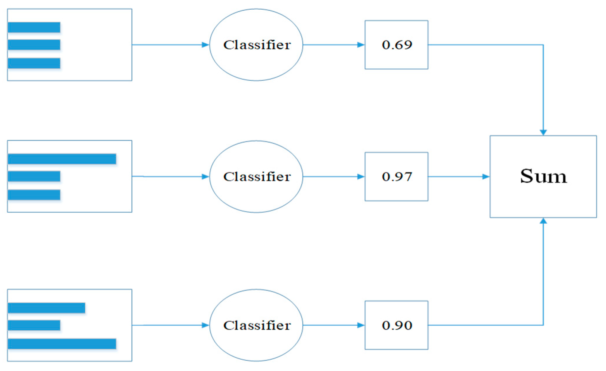
The selected supervised classifiers are the random forests (RF), adaptive boosting (AdaBoost) and classification and regression tree (CART). The CART algorithm, a decision tree model and a non-parametric data mining method, has many advantages including ease of handling numerical and categorical data and multiple outputs situations [25]. The CART algorithm is a component learner with gini features, such as division standard, while ensemble learning combines multiple weak classifiers using different methods. The most common methods of ensemble learning are bootstrap aggregating (bagging) method and boosting method, in which bagging is a parallel algorithm and boosting is a sequential algorithm. The RF algorithm, the expansion of bagging method, exploits random binary trees to discriminate and classify data [7]. The AdaBoost approach, a boosting algorithm, constructs a strong classifier with weak classifiers and updates the weight of samples based on learning error, as shown in Figure 2. Each sample in the training data is given equal weight α at first. A weak classifier is trained on the training data and the error rate ε of the classifier is calculated. Then, the classifier is trained again on the unified data. The ε will be increased while αwill be reduced to the first classification on the second training classifier. AdaBoost calculates ε of each weak classifier and assigns α to each classifier. In Figure 2, the first row is the data set, where the different width of histograms represents different weight on each sample. The data set will be weighted by α in the third row after passing through the classifier [26]. The final output is obtained by summing the weighted results. The the error rate ε (Equation (1)) and the weight α (Equation (2)) are calculated as follows:

$$\mathsf{\epsilon }=\frac{N1}{N2}$$

(1)

$$\mathsf{\alpha }=\frac{1}{2}\left(\frac{1-\epsilon }{\epsilon }\right)$$

(2)

where N1, N2 are the number of incorrectly classified and classified samples, respectively.

We worked with the CART, RF, and AdaBoost models implemented in the jupyter of the Anaconda Navigator. Data was generally required to be standardized in machine learning. We used the StandardScaler preprocessing method of the sklearn function library to process the magnitude, focal depth, epicentral intensity, and population density. Equation (3) presents the process:

$$\mathrm{x}=\left(\mathrm{x}-\mathsf{\mu }\right)/\mathsf{\sigma }$$

(3)

where x is the features, μ is the mean of the data and δ is the variance of the data. The parameters selection of each model is shown in

Table 2. Parameters of random forest (RF), CART, and AdaBoost (Unset parameters were used as default parameters in sklearn, AdaBoost has two classes of classification algorithms SAMME and SAMME.R, among which SAMME.R is better based on class probability).

Random Forest	CART	AdaBoost
number of estimators = 82 number of jobs = −1 max features = none criterion = gini	max depth = 10 max features = none number of estimators = 500 criterion = gini	base estimator = decision trees classifier algorithm = SAMME.R learning rate = 0.5 number of estimators = 379

.

Table 3. Results of testing the models on unseen validation set of 9 features.

Algorithm	Random Forest	CART	AdaBoost
Mean accuracy	0.820	0.745	0.766

presents the result of verifying the model with cross validation score function in sklearn function library. And the importance of nine features in casualty assessment is shown in Figure 3.

2.3. Importance Assessments of Structure Types

The importance of different structure types was assessed alone because of the complexity of the structure types and the great contribution to the death [27]. For the accuracy and comprehensiveness of the assessment, this study listed 43 universal and special structure types from the Earthquake Disasters and Losses Assessment Report in Chinese Mainland from 1992 to 2007: reinforced concrete frame structure, masonry structure, brick-wood structure, civil structure, national brick-wood structure, brick-concrete structure, bucket-piercing frame structure, brick-concrete structure (building of two or more floors), shed, brick-concrete structure(building of only one floor), brick-column civil structure, wing-room, national civil structure, simple house with dry fortified earth wall, brick-column adobe structure, dry brick building, brick structure, timber structure, timber stack structure, timber framework, brick-masonry structure, frame structure, adobe structure, wood-column adobe structure, reinforced frame structure, mixed house, brick adobe structure, general houses (owned by citizens), stone-wood structure, stone structure, simple house, old Tibetan house, stone-grass structure, stone-concrete structure, alunite house, earth rock house, industrial plant, steel frame structure, soil tamper structure, cave dwelling, wooden frame house, flag stone house, and general house.

Structural damages were divided into five grades: collapse, heavy damage, moderate damage, slight damage, and basically undamaged. We chose the collapse, heavy damage of buildings, and population density as input parameters. Firstly, death was almost being caused by the collapse and heavy damage of the architecture. Another, population density, was closely related to the seismic casualty and the number of buildings. We only selected random forest algorithm to assess the importance of structure types for the mean accuracy of the RF model was higher than the other algorithm as seen from Table 3.

Table 4. Steps of the random forest algorithm.

Step by Step Procedure of Random Forests Algorithm

Inputs: a, b, c, d a: Damage ratio of collapse of different structures b: Damage ratio of heavy damage of different structures c: Population density d: Death Parameters: number of estimators = 500, criterion = gini, numbers of jobs = -1, max features = None, criterion = MSE, max depth = None, max leaf nodes = None, min impurity decrease = 0.0, min impurity split = None, min samples leaf = 1, min samples split = 2, min weight fraction leaf = 0.0, presort = False, random state = None, splitter = best Process: step1: Bootstrap sampling is used to extract sub-training sets from the training set. step2: Generate the feature subsets by randomly selecting features before node splits. step3: Establish decision trees step4: Obtain the results for the sample to be tested step5: Vote on the results and got the results. Output: Importance of structure types

presents the procedure of RF in feature assessment. The importance of structure types can be seen in Figure 4.

3. Model

We chose the population density, magnitude, focal depth, epicentral intensity, and time as the input parameters. The criteria and reasons for selecting five input parameters among ten features were as follows:

(1)

Features were selected from high to low in the order of features importance. According to their subjectivity, the number of occurrences and obtained time after the earthquake.

(2)

The results of the importance assessment show the relative values of the nine factors that contribute to the assessment of the casualty, rather than the absolute value of each of the factors alone. Time ranked seventh instead of higher in the importance assessment results because we only divided it into the two parts. In the deep learning model, we did not to classify the time. Therefore, we chose the time because it could be almost obtained at the same time as an earthquake and it had not subjectivity in the deep learning model.

(3)

The division of the economic status had a strong subjectivity and the data selected in the test set was the economic situation of the year of the occurrence of the earthquake. With the annual inflation and the depreciation of the coin, the situation of that year may not be applicable to the future.

(4)

Although the date was more important than the time, the subjectivity of the date was also great, which was only divided into four seasons.

(5)

The secondary disasters and abnormal intensity were only divided into yes and no. The combined number of the two phenomena was small and not every earthquake was accompanied by them.

(6)

The structure types were too complex. Structure destroyed during each earthquake were different and every destruction was divided into five parts.

3.1. Data

We collected 289 destructive earthquakes occurred in the Chinese mainland from 1992 to 2017 in the Earthquake Disasters and Losses Assessment Report in Chinese Mainland (

Table A1. The 289 earthquake cases of the deep learning model with the default value from 1992 to 2017 in China mainland.

	Date	Time	Magnitude (Ms)	Epicentral Intensity	Focal Depth (km)	Population Density (People Per Square)	Deaths
1	1992/4/23	11:32 PM	6.9	7		64.98	4
2	1992/12/18	7:21 PM	5.4	6		311.11	1
3	1993/1/27	4:32 AM	6.3	8	14	60.68	0
4	1993/2/1	3:33 AM	5.3	6	10	35.63	0
5	1993/3/20	10:52 PM	6.6	8		11.76	2
6	1993/5/24	7:57 AM	5	6		21.28	0
7	1993/5/30	3:26 PM	4.9	6	10	122.38	0
8	1993/7/17	5:46 PM	5.6	6	16	11.06	1
9	1993/8/14	10:30 PM	5.6	7	8	105.60	0
10	1993/9/5	4:22AM	5.1	6	40	32.33	0
11	1993/12/1	4:37 AM	6	7	28	94.26	2
12	1994/1/11	8:51 AM	6.7	7	10	16.45	0
13	1994/9/16	2:20 PM	7.3	7	20	700.00	4
14	1994/9/19	11:28 PM	5.2	6		197.35	0
15	1995/2/18	8:14 AM	5.1	6		101.51	0
16	1995/4/25	12:13 AM	5.6	7	20	62.42	0
17	1995/7/12	5:46 AM	7.3	8	10	55.50	11
18	1995/7/22	6:44 AM	5.8	8	10	80.31	12
19	1995/9/20	11:14 AM	5.2	6	12		0
20	1995/9/26	12:39 PM	5.3	6	27	11.62	0
21	1995/10/6	6:26 AM	4.9	6	10	945.95	0
22	1995/10/24	6:46 AM	6.5	9	12.5	81.94	59
23	1996/2/3	7:14 PM	7	9	10	57.44	309
24	1996/2/28	7:21 PM	5.4	7	15	412.94	1
25	1996/3/19	11:00 PM	6.9	8	11	3.38	24
26	1996/5/3	11:32 AM	6.4	8	24	183.19	26
27	1996/6/1	8:49 PM	5.4	6	10	91.97	0
28	1996/7/2	3:05 PM	5.2	6	10	125.55	2
29	1996/9/25	3:24 AM	5.7	7	15	42.56	1
30	1996/12/21	4:39 PM	5.5	7		5.16	2
31	1997/1/21	9:47 AM	6.4	8		180.59	12
32	1997/1/25	10:38 AM	5.1	6	10	3.03	0
33	1997/1/30	5:59 PM	5.5	7	10	36.82	0
34	1997/3/1	2:04 PM	6	7		131.98	1
35	1997/4/11	1:34 PM	6.6	8	17	58.78	8
36	1997/5/31	2:51 PM	5.2	6		76.28	0
37	1997/8/13	4:13 PM	5.3	7	7.9	545.09	0
38	1997/9/26	11:19 AM	4.2	6	4.8	314.60	0
39	1997/10/23	8:28 PM	5.3	6	10	587.57	0
40	1997/11/3	10:29 AM	5.6	7	14	0.93
41	1998/1/10	11:50 AM	6.2	8	10	82.11	49
42	1998/3/19	9:51 PM	6	7	11	6.75	0
43	1998/4/14	10:47 AM	4.7	6	10.7	0.00	0
44	1998/5/29	5:11 AM	6.2	7	11	19.09	0
45	1998/6/25	2:39 PM	5.2	5	11	926.69	1
46	1998/7/11	7:04 PM	5	6	15.5	17.03	0
47	1998/7/20	9:05 AM	6.1	7	14	3.59
48	1998/7/28	12:51 PM	5.5	6	11	25.28	0
49	1998/8/27	5:03 PM	6.6	8	11	42.09	3
50	1998/9/18	11:53 AM	4.8	6	15	361.84	0
51	1998/10/2	8:49 PM	5.3	7	13	83.46	0
52	1998/11/19	7:38 PM	6.2	8	10	40.22	6
53	1998/12/1	3:37 PM	5.1	7	10	322.07	0
54	1999/3/11	9:18 PM	5.6	7	11	116.08	0
55	1999/3/15	6:42 PM	5.6	6	11	16.93	0
56	1999/4/15	2:29 PM	4.7	6	8	88.60	1
57	1999/5/17	11:29 AM	5.2	6	20	471.60	0
58	1999/6/17	11:02 PM	5.3	5	11	25.28	0
59	1999/8/17	6:47 PM	5	7	12	5413.56	0
60	1999/9/14	8:54 PM	5	6	9	91.67	0
61	1999/9/27	7:49 PM	5.1	6	20	14.14	0
62	1999/11/1	9:24 PM	5.6	7	9	271.87	0
63	1999/11/25	12:40 AM	5.2	6	10	314.93	1
64	1999/11/26	4:51 AM	5	6	13	15.07	0
65	1999/11/29	12:10 PM	5.6	7	15	27.03
66	1999/11/30	4:24 PM	5	6	26	651.86	1
67	2000/1/15	7:37 AM	6.5	6	30	123.04	7
68	2000/1/27	4:55 AM	5.5	7	10	115.12	0
69	2000/4/15	5:32 PM	5.3	7	13	1.19	0
70	2000/4/29	11:54 AM	4.7	6	16	10.33	1
71	2000/6/6	6:59 PM	5.9	8	15	247.06	0
72	2000/8/21	9:25 PM	5.1	6	8	87.61	2
73	2000/9/12	8:27 AM	6.6	8	13	4.55	0
74	2000/10/6	8:05 PM	5.8	6	18	147.33	0
75	2001/2/23	8:09 AM	6			4.70	3
76	2001/3/12	4:57 PM	5	6	10	103.06	0
77	2001/3/24	7:23 AM	5	5		3.63	0
78	2001/4/12	11:13 AM	5.9	8	6	196.15	2
79	2001/5/24	5:10 AM	5.8	7	5	39.07	1
80	2001/5/24	5:10 AM	5.8	7	5	99.64	0
81	2001/6/8	2:03 AM	5.3	6	5	208.09	1
82	2001/6/23	10:48 AM	4.9	6	15.4	4736.80	0
83	2001/7/10	7:51 AM	5.3	6	13	125.50	0
84	2001/7/11	5:41 AM	5.3	6	10	8.32	0
85	2001/7/15	2:36 AM	5.1	6	8	337.43	0
86	2001/9/4	12:05 PM	5	6	8	102.91	0
87	2001/10/27	1:35 PM	6	7	15	138.41	1
88	2001/11/14	5:26 PM	8.1	10			0
89	2002/8/8	7:42 PM	5.3	7		7.63	0
90	2002/9/5	12:18 PM	4	6		185.70	0
91	2002/10/20	11:46 PM	5	6	15	19.15	0
92	2002/12/14	9:27 PM	5.9	7	15	7.35	2
93	2002/12/25	8:57 PM	5.7	6	20	5.28	0
94	2003/1/4	7:07 PM	5.4	6	17	124.75	0
95	2003/2/14	1:34 AM	5.4	6	25		0
96	2003/2/24	10:03 AM	6.8	9	25.2	30.67	268
97	2003/4/17	8:48 AM	6.6	8	14	3.84	0
98	2003/4/24	6:37 AM	4.5	6	12	56.53	0
99	2003/5/4	11:44 PM	5.8	7	26.7	49.29	1
100	2003/6/17	10:46 PM	4.8	5	5	172.20	0
101	2003/7/10	9:54 AM	4.8	6	10	241.69	0
102	2003/7/21	11:16 PM	6.2	8	6	101.91	16
103	2003/8/16	6:58 PM	5.9	8	15	36.46	4
104	2003/8/18	5:03 PM	5.7	7	9	3.08	2
105	2003/8/21	10:16 AM	5	6	10	2287.92	0
106	2003/9/2	7:16 AM	5.9	6	10	1.77	0
107	2003/9/27	7:33 PM	7.9	11	15	5.48	0
108	2003/10/16	6:28 PM	6.1	8	5	84.30	3
109	2003/10/25	8:41 PM	6.1	8	18	58.87	10
110	2003/11/13	10:35 AM	5.2	8	12	165.95	1
111	2003/11/15	2:49 AM	5.1	7	10	415.91	4
112	2003/11/25	1:40 PM	4.9	6	20	27.87	0
113	2003/11/26	9:38 PM	5	7	8	411.22	0
114	2003/12/1	9:38 AM	6.1	8	18	20.68	10
115	2004/3/7	9:29 PM	5.6	6	15	2.43	0
116	2004/3/24	9:53 AM	5.9	7	30	2.91	1
117	2004/5/11	7:27 AM	5.9		20	2.34	0
118	2004/6/17	5:25 AM	4.7	6	5	322.13	1
119	2004/7/12	7:08 AM	6.7		33	0.45	0
120	2004/8/10	6:26 PM	5.6	8	10	353.50	4
121	2004/8/24	6:05 PM	5.8		25	1.11	0
122	2004/9/7	8:15 PM	5	7	33	105.80	1
123	2004/9/17	2:31 AM	4.9	6	12	295.74	0
124	2004/10/19	6:11 AM	5	6	6	899.16	0
125	2004/12/26	3:30 PM	5	6	7	72.44	1
126	2005/1/5	6:05 AM	4.7	6	5	6.32	0
127	2005/1/26	12:30 AM	5	6	6	69.30	0
128	2005/2/15	7:38 AM	6.2	7	32	38.81	0
129	2005/4/8	4:04 AM	6.5	6	10	21.14	0
130	2005/6/2	4:06 AM	5.9	6		6.37	0
131	2005/7/25	11:43 PM	5.1	6	15	88.85	1
132	2005/8/5	10:14 PM	5.3	6	21	178.52	0
133	2005/8/13	12:58 PM	5.3	6	15	143.40	0
134	2005/8/26	5:08 AM	5.2	6		2.27	0
135	2005/10/27	7:18 PM	4.4	6	16	152.50	1
136	2005/11/26	8:49 AM	5.7	7	10	638.10	13
137	2006/1/12	9:05 AM	5	6	16	83.14	0
138	2006/3/27	3:20 AM	4.3	6	14	0.00	0
139	2006/3/31	8:23 PM	5	6	15	54.31	0
140	2006/6/21	12:52 AM	5	6	15	93.70	1
141	2006/7/4	11:56 AM	5.1	5	20	437.74	0
142	2006/7/19	5:53 PM	5.6	7	15	4.90	0
143	2006/7/22	9:10 AM	5.1	6	9	169.85	22
144	2006/8/25	1:51 PM	5.1	7	7	194.47	2
145	2006/11/23	10:04 AM	5.1	5	17		0
146	2007/3/13	10:22 AM	4.9	6	6	2175.44	0
147	2007/6/3	5:34 AM	6.4	8	5	103.63	3
148	2007/6/23	4:17 PM	5.8	6	16	94.32	0
149	2007/7/20	6:06 PM	5.7	7	25	27.43	0
150	2008/2/1	5:06 AM	4.6	6	6	496.13	0
151	2008/3/21	6:33 AM	7.3	7	33	14.39	0
152	2008/3/21	8:36 PM	5	6	11	157.98	0
153	2008/3/24	11:24 PM	4.1	6	10	1000.00	0
154	2008/3/30	4:32 PM	5	6	33	26.15	0
155	2008/4/20	9:14 PM	5.1	6	22	62.46	0
156	2008/4/21	5:42 AM	4.2	6	33	26.15	0
157	2008/5/12	2:28 PM	8	9	14	238.34	69227
158	2008/6/10	2:05 PM	5.2	6	14	4.20	0
159	2008/8/21	8:24 PM	5.9	8	7	78.78	5
160	2008/8/30	4:30 PM	6.1	8	10	131.52	41
161	2008/8/30	8:46 PM	5.3	6	25	2.85	0
162	2008/10/5	11:52 PM	6.8	8	27	3.62	0
163	2008/10/6	4:30 PM	6.6	8	8	10.17	10
164	2008/11/10	9:22 AM	6.3	7	10	9.25	0
165	2008/11/22	4:01 PM	4.1	6	8	200.00	0
166	2008/12/26	4:20 AM	4.9	6	5	399.36	0
167	2009/1/25	9:47 AM	5	6	7	14.41	0
168	2009/2/20	6:02 PM	5.2	6	6	15.22	0
169	2009/4/19	12:08 PM	5.5	6	7	8.45	0
170	2009/4/22	5:26 PM	5	6	7	6.24	0
171	2009/7/9	7:19 PM	6	8	10	115.44	1
172	2009/8/8	9:26 PM	4	6	11	1885.35	2
173	2009/8/28	9:52 AM	6.4	7	8	2.36	0
174	2009/11/2	5:07 AM	5	6	10	117.18	0
175	2010/1/17	5:37 PM	3.4		7		6
176	2010/1/31	5:36 AM	5	7	10	1661.60	1
177	2010/2/22	9:32 PM	4.2	6	10	51.52	0
178	2010/2/25	12:56 PM	5.1	6	16	105.26	0
179	2010/4/4	9:46 PM	4.5	5	8	38.20	0
180	2010/4/14	7:49 AM	7.1	9	14	8.69	2698
181	2010/6/5	8:58 PM	4.6	5	5	5.76	1
182	2010/6/10	2:38 PM	5.1	6	8	0.93	0
183	2010/8/29	8:53 AM	4.8				0
184	2010/10/24	4:58 PM	4.7	6	8	714.98	0
185	2011/1/1	9:56 AM	5.1		10
186	2011/1/8	7:34 AM	5.6		560
187	2011/1/12	9:19 AM	5		10
188	2011/1/19	12:07 PM	4.8	6	9	1749.16	0
189	2011/2/1	4:16 PM	5.3		7
190	2011/2/15	3:18 PM	5.1		10
191	2011/3/10	12:58 PM	5.8	8	10	84.55	25
192	2011/3/20	4:00 PM	5.2		30
193	2011/3/24	9:55 PM	7.2	6	20	58.67	0
194	2011/4/10	5:02 PM	5.3	7	7	10.96	0
195	2011/4/16	9:11 AM	6		130
196	2011/4/30	4:35 PM	5		60
197	2011/5/10	11:41 PM	6.1		560
198	2011/5/22	9:34 AM	5.2		10
199	2011/6/8	9:53 AM	5.3	6	5	0.02	0
200	2011/6/20	6:16 PM	5.2	6	10	139.08	0
201	2011/6/26	3:48 PM	5.2		10	235.26	0
202	2011/7/25	3:05 AM	5.2	6	10	6.02	0
203	2011/8/2	3:40 AM	5.1		10
204	2011/8/9	7:50 PM	5.2		11	134.75	0
205	2011/8/11	6:06 PM	5.8	7	8	19.71	0
206	2011/9/15	11:27 PM	5.5	6	6	1.75	0
207	2011/9/18	8:40 PM	6.8	7	20	3.51	7
208	2011/10/16	9:44 PM	5	6	4	11.29	0
209	2011/10/30	11:23 AM	5.7		223
210	2011/11/1	5:58 AM	5.4		20
211	2011/11/1	8:21 AM	6	7	28	45.00	0
212	2011/12/1	8:48 PM	5.2	6	10	104.13	0
213	2012/1/8	2:20 PM	5	6	27	24.52	0
214	2012/3/9	6:50 AM	6		30	1.18	0
215	2012/5/3	6:19 PM	5.4	7	8	7.78	0
216	2012/6/15	5:51 AM	5.4	6	20	9.38	0
217	2012/6/24	3:59 PM	5.7	7	11	52.39	4
218	2012/6/30	5:07 AM	6.6	8	10	13.60	0
219	2012/7/20	8:11 PM	4.9	6	6	640.63	1
220	2012/8/12	6:47 PM	6.2	7	30	2.62	0
221	2012/9/7	11:19 AM	5.7	8	14	226.83	81
222	2012/11/26	1:33 PM	5.5	6	8	93.75	0
223	2012/12/7	10:08 PM	5.1	6	9	7.29	0
224	2013/1/18	8:42 PM	5.4	7	15	11.90	0
225	2013/1/23	12:18 PM	5.1	6	7	625.00
226	2013/1/24	2:01 AM	4.2	5
227	2013/1/29	12:38 AM	6.1	7	20	16.34	0
228	2013/3/3	1:41 PM	5.5	7	9	68.04	0
229	2013/3/11	11:01 AM	5.2	6	8	42.24	0
230	2013/3/29	1:01 PM	5.6	6	13	5.23	0
231	2013/4/17	9:45 AM	5	7	9	68.87	0
232	2013/4/20	8:02 AM	7	9	13	116.88	196
233	2013/4/22	5:11 PM	5.3	7	6	106.99	2
234	2013/7/22	7:45 AM	6.6	8	20	139.97	95
235	2013/8/12	5:23 AM	6.1	8	10	13.04
236	2013/8/28	4:44 AM	5.1	8	9	15.75	3
237	2013/8/31	8:04 AM	5.9	8	10	3.57	3
238	2013/11/23	6:04 AM	5.5	7	9
239	2013/12/1	4:34 PM	5.3	6	9	29.01	0
240	2013/12/16	1:04 PM	5.1	7	5	147.91	0
241	2014/2/12	5:19 PM	7.3	9	12	3.39	0
242	2014/4/5	6:40 AM	5.3	6	13	274.05	0
243	2014/5/30	9:20 AM	6.1	8	12	87.12
244	2014/8/3	4:30 PM	6.5	9	12	216.67	617
245	2014/8/17	6:07 AM	5	6	7	325.71
246	2014/10/1	9:23 AM	5	6	15	30.23	0
247	2014/10/7	9:49 PM	6.6	8	5	48.25	1
248	2014/10/25	1:20 PM	4.2	6	5	1611.89	0
249	2014/11/22	4:55 PM	6.3	8	18	16.72	5
250	2014/12/6	4:20 PM	5.9	8	10	48.25	1
251	2015/1/10	2:50 PM	5	5	10	2.69	0
252	2015/1/14	1:21 PM	5	6	14	164.58	0
253	2015/2/22	2:42 PM	5	6	14	171.79	0
254	2015/3/1	6:24 PM	5.5	7	11	70.81	0
255	2015/3/14	6:14 AM	4.3	6	10	7625.50	2
256	2015/3/30	9:47 AM	5.5	7	7	119.03	0
257	2015/4/15	7:08 AM	4.5	6	9	144.31	1
258	2015/4/15	3:39 PM	5.8	7	10	4.56	0
259	2015/4/25	2:11 PM	8.1	9	20	4.33	27
260	2015/5/22	12:05 AM	4.6	5	7		0
261	2015/7/3	9:07 AM	6.5	8	10	44.83	3
262	2015/10/30	7:26 PM	5.1	6	10	62.39	0
263	2016/1/14	5:18 AM	5.3	6	5	8.22	0
264	2016/1/21	1:13 AM	6.4	8	10	0.64	0
265	2016/2/11	9:10 PM	5	6	8	3.81	0
266	2016/3/12	11:14 AM	4.4	6	5		0
267	2016/5/11	9:15 AM	5.5	7	6.9		0
268	2016/5/18	12:48 AM	5	6	15	7.49	0
269	2016/5/22	5:08 PM	4.6	6	6	162.50	0
270	2016/7/31	5:18 PM	5.4	7	10	21.98	0
271	2016/8/11	11:49 AM	4.4	5	10	13.15	0
272	2016/9/23	1:23 AM	5.1	6	16	35.77	0
273	2016/10/17	3:14 PM	6.2	7	9	21.83	1
274	2016/11/25	10:24 PM	6.7	8	10	0.65	1
275	2016/12/8	1:15 PM	6.2	8	6	3.10	0
276	2016/12/14	4:14 PM	5		5		0
277	2016/12/20	6:04 PM	5.8	7	9	0.73	0
278	2016/12/27	8:17 AM	4.8	6	10		0
279	2017/1/28	2:46 AM	4.9	6	11		0
280	2017/2/8	7:11 PM	4.9	7	10		0
281	2017/3/27	7:55 AM	5.1	6	12	58.29	0
282	2017/5/4	1:40 PM	4.9	6	10		0
283	2017/5/11	5:58 AM	5.5	7	8	16.64	8
284	2017/6/16	7:48 PM	4.3	7	5	20.77	0
285	2017/8/18	9:19 PM	7	9	20	28.79	30
286	2017/8/9	7:27 AM	6.6	8	11	169.66	0
287	2017/9/30	2:14 PM	5.4	6	13	3.62	0
288	2017/11/18	6:34 AM	6.9	8	10		0
289	2017/11/23	5:43 PM	5	6	10		0

). The excel table data were pre-processed by openpyxl module in deep learning method, and the data set of 228 earthquake cases were returned without a missing value. Among these data, we selected 180 data as the training set and 38 data as the test set. The remaining ten were used as validation sets. The time was recorded in minutes, and the hours are converted into minutes, which are calculated at 1440 min per day. When the time is x: y, the data will be processed as (60x+y)/144. For example, if the time is 04:32, the change is 0.19. Other parameters need not be specially processed.

3.2. Deep Learning Model

3.2.1. Hyper Parameter

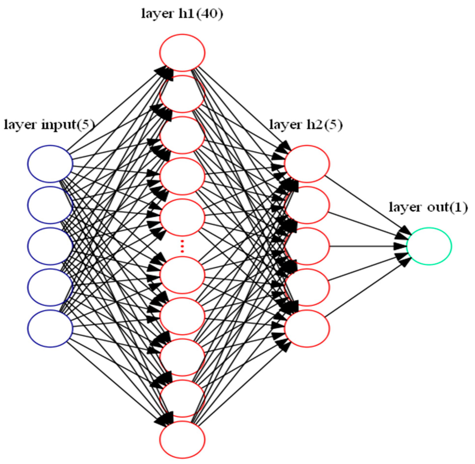
A deep learning model is a multilayer stack of simple modules and many of which compute non-linear input to output mappings. The hidden layers of 3 to 18 in the deep learning model can implement extremely complex functions of the original variables that are sensitive to minute details [23]. Given the small data set in this study, we chose a four-layers back propagation network. The number of neurons in the hidden layers was optimized for getting accurate output [21]. To select the number of two hidden layer’s neurons, the training began with ten and three neurons separately and was repeated for more neurons. The number of neurons in the hidden layers were determined to be 40 and 5 separately for reducing the complexity and running time of the model.

There are different methods to avoid over fitting during the training process and to obtain models that are expert in generalizing the problem to be explained. For instance, stopping iteration in advance, regularization, dropout, and data set expansion. Stopping iteration in advance and data set expansion are not applicable to this model. The dropout method is a random deletion of half of the hidden layer nodes, hence, it is also not applicable. Finally, the regularization method was chosen. Regularization in deep learning includes coefficients L1 and L2. We chose the most commonly used L2 regularization. L2 regularization is to add an additional regularization term to the loss function, presented in Equation (4).

$$\mathrm{c}=c_0+\frac{\lambda }{2n}{\displaystyle \sum _w}{w}^2$$

(4)

where c and c₀ are the new and old loss functions, separately, λ is the L2 regularization rate, n is the number of the sample and w is the weight. Through a large number of tests, the optimal parameters were obtained as shown in

Table 5. Hyper parameters.

Batch Size	Learning Rate Base	Learning Rate Decay	Regularization Rate	Training Steps	Moving Average Decay
16	0.8	0.99	0.00005	500000	0.99

. Figure 5 demonstrates the model with two hidden layers, consisting of forty and five neurons respectively, five input layers, and one output layer.

3.2.2. Optimization Algorithm

The optimization algorithms used in the model including the adaptive moment estimation (Adam) [28], mini-batch gradient descent [29], and moving average model [30]. We used the adam algorithm to make the learning rates updating independent for parameters by calculating the first and second moment estimation of gradients. The mini-batch is to reduce the randomness for the data in a pool determine the direction of the gradient together and reduce the possibility of deviation during the descent process [31]. The model computer was a workstation with a good performance and the data volume of the model was less than 2000. The size of the training pool was usually chosen as the n-th power of 2. Hence, we chose 16 data as a training pool through experiments. The moving average model is to prevent the sudden change when updating parameters [32].

3.2.3. Process of the Model

Definition structure and forward propagation used tensorflow framework [30]. The parameters of deep learning network needed only define weights w and b, and the normal distribution was chosen as the weight generating function. The activation function was relu function [23] and was used in the first hidden layer. The second hidden layer and the output layer are basically equivalent to linear regression. We selected Adam algorithm as back propagation algorithm. The learning rate is optimized. The mean square error loss function was selected for the data set was little (Equation (5)).

$$\mathrm{c}=\frac{1}{n}\sum {\left(y-t\right)}^2$$

(5)

where c presents loss function, n is the number of the samples, y is the predictive value and t is the true value.

4. Results

We chose ten seismic cases with different parameters as the test data, of which the eighth, ninth, and tenth cases were Ludian earthquake in 2014, Yushu earthquake in 2010 and Wenchuan earthquake in 2008. Selection of specific test sets is shown in

Table 6. Test sets.

Number	Time	Magnitude (Ms.)	Epicentral Intensity (Degree)	Focal Depth (km)	Population Density (People/km2)
1	0.33	5.1	6	12	58.28519
2	0.84	5.0	7	33	105.7979
3	0.25	5.5	7	8	16.63824
4	0.38	5.1	6	9	169.8517
5	0.96	6.9	8	11	3.384553
6	0.69	6.1	8	10	131.524
7	0.47	5.7	8	14	226.8326
8	0.69	6.5	9	12	216.6675
9	0.33	7.1	9	14	8.686792
10	0.60	8.0	11	14	238.3409

. Comparing with the intensity-based mortality estimation method in Assessment of Earthquake Disaster Situation in Emergency Period [33] (China-National Standard), presented in Equation (6) and (7). The Standard is an important basis for the government’s decision-making on earthquake relief. After an earthquake, the primary tasks of the emergency work are to conduct disaster investigation and assessment in a short period of time and to provide the government with timely and necessary information on the disaster situation. Therefore, relevant departments have formulated the Standard in a comprehensive summary of the research methods and field practices of earthquake disaster assessment in China. Focus on rapid and dynamic disaster recovery and assessment.

$$N_D={\sum }_{j=6}^{I_{max}}{A}_j\rho R_j$$

(6)

$$\ln R_j=-44.365+7.516I_j-0.329I_j^2$$

(7)

where N_D is the number of deaths; I_max is the intensity of the meizoseismal area; A_j is the distribution area of intensity value j; ρ is the population density; R_j is the death rate corresponding to the intensity value j; I_j is the intensity value j.

Table 7. Comparison results.

Number	Deep Learning	China-National Standard	True Value
1	0	0	0
2	0	0	1
3	7	0	8
4	26	0	22
5	24	0	24
6	36	10	41
7	80	18	81
8	245	173	617
9	2625	7	2698
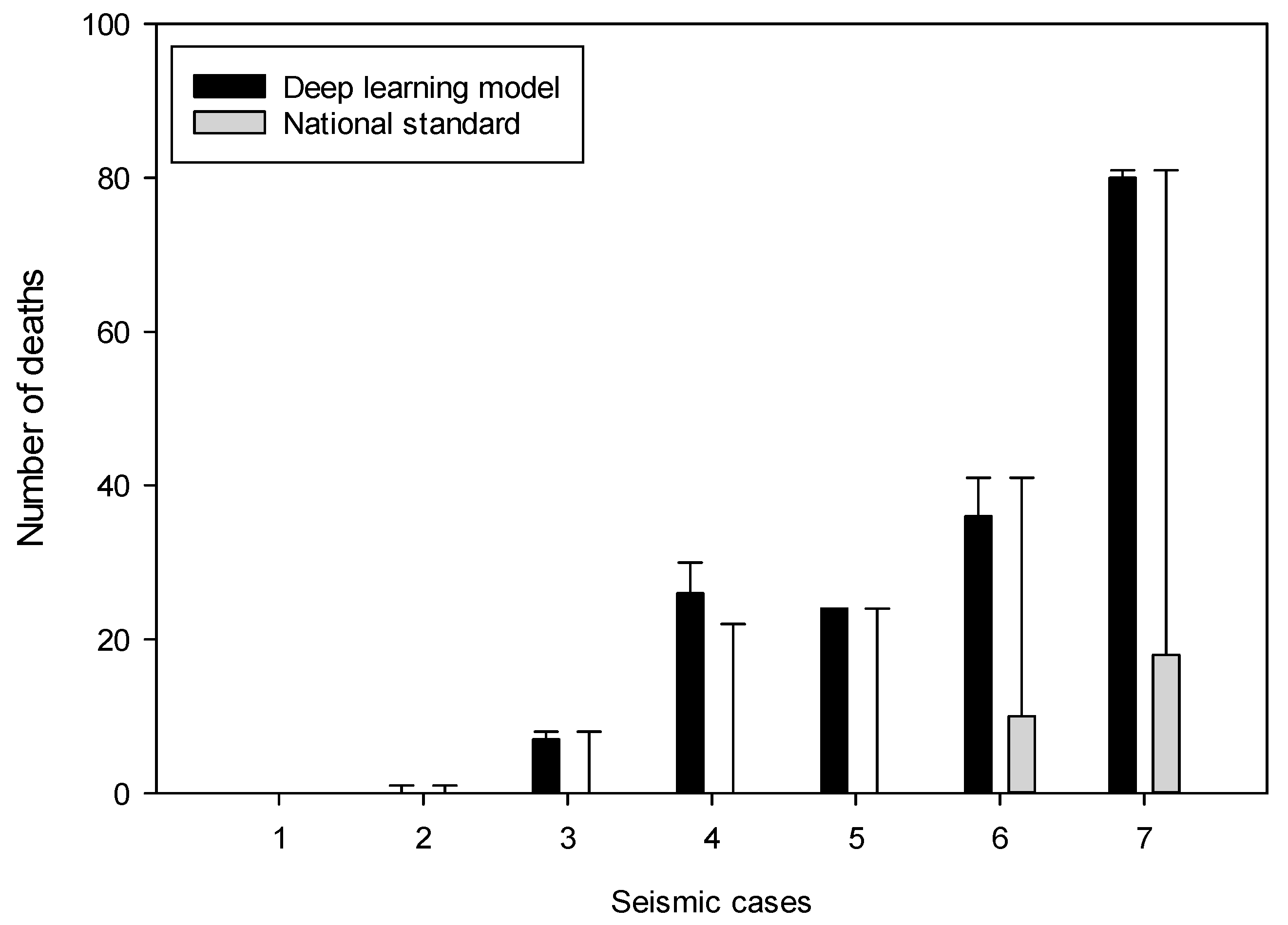
10	37406	191	69227

and Figure 6 show the comparison results of the deep learning model, China-National Standard and true value.

Table 8. The accuracy of two models.

Method	Cases 1–7	Cases 8–10	Cases 1–10
China-National Standard	52.27%	25.32%	44.19%
Deep learning model	93.61%	45.85%	79.28%

presents the accuracy of the two methods in cases from1 to 7 and cases from 8 to 10, separately. The results demonstrate as follows:

(1)

Adam algorithm and moving average model based on deep learning can accelerate the convergence speed and improve the accuracy of model prediction.

(2)

The accuracy was higher, and the factors considered were more than the Standard.

(3)

The prediction accuracy of the last three earthquake cases is generally not high.

(4)

The China-National Standard model selected fewer parameters. The model was based on the experience of many experts and had been tested for many years. In the cases 1–7, the predicted values and the true values were all on the order of magnitude, but the performance on the cases 8–10 was far worse than the deep learning model, which was far from the true value and has no reference for the actual earthquakes.

5. Discussion

Three issues were considered in this study: the importance of nine features to the human losses in China mainland, the importance of 43 structure types of the fatalities, and human losses assessment. The first issue was addressed by adopting three traditional machine learning method domains to investigate different features’ influence on the seismic fatalities. The results can provide a basis for further seismic assessment. The second issue was addressed by RF algorithm to assess the importance of 43 structure types. The third issue was addressed by establishing a deep learning model domain to predict the seismic death. A detailed investigation of these two issues is presented as follows.

5.1. Importance of Different Features

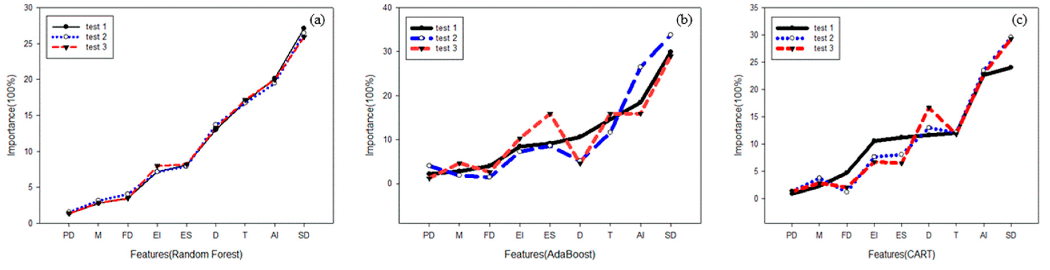
We propose an automatic classifier based on RF, CART, and AdaBoost, and some attributes to describe the feature importance of seismic. Random forest is the most stable among three methods. Figure 7 exhibits the results of three tests on that three methods. RF provides probability estimates on the classification that are useful to accept or reject a new classification [8]. Thus, we chose the RF algorithm as the main method. It fully proved the importance of the population density, magnitude, focal depth, epicentral intensity. The sum of the four features is 74.68%, which is far more important than other factors.

Time is vital to seismic, for example, the Tangshan earthquake occurred at 3:24 on July 28, 1976, when people slept in the house, and time aggravated the disaster. Losses will be relatively mitigated in daytime for most people are not sleeping and could escape quickly. The reason that time ranks seventh in this study is that time was only divided into two possibilities: daytime and sleeping time. More classes are discriminated by an attribute, the more important the attribute is [8]. In the same way, the ratio of abnormal intensity and the secondary disaster are only 2.63% and 1.18% separately for the fewer classes. However, time is divided into different levels, not modeled at an actual time, so there is interference with the results. The secondary disasters and the abnormal intensity are classified because they occur less frequently. In summary, the features selected by the RF algorithm experiments are consistent with those used by other scholars to study earthquake casualties (population density [2], magnitude [2], focal depth [34], epicentral intensity [16], and time [13]).

5.2. Importance of Different Structure Types

We chose all 43 structure types in China mainland to assess, which are far more than the number of the types in the previous studies [35]. Although the structure types of the WHE project are suitable for the most region of the world, it also lacks some structures that Chinese characteristic structure, such as the national civil structure, the old Tibetan house and the national brick-wood structure. Hence, the data from the Earthquake Disasters and Losses Assessment Report in Chinese Mainland of every earthquake in China mainland is more suitable for the study comparing the data of the WHE project. The HAZUS system (HAZad United States of Multi-Hazard) only has twelve structure types and estimates the casualties for collapsed buildings and not for the heavy damaged buildings [18]. In reference [18], the casualties are estimated at the level of single buildings and not for an entire zone in an adapted HAZUS system. The population density varies greatly in different parts of China, so the HAZUS system and the adapted system are not suitable for the casualties estimation of China.

The importance of different structural types was obtained based on RF method first. In the part of data collecting, there are no integration of structural forms and some may be slightly repeated in order not to omit any structure type. For instance, brick-column civil structure, brick-concrete structure (building of two or more floors) and brick-concrete structure (building of only one floor). However, repeated structures, even when combined, the importance was close to zero.

Figure 4 displays that the contribution to the casualties of reinforced concrete structure is the largest, followed by civil structure, stone-concrete structure, brick-concrete structure, brick-wood structure, brick house and the frame house. The other structures are not shown in Figure 4 and could be neglected. We concluded that the structure with large effect may not be good at seismic behavior. The result manifests that once the building is destroyed, the damage will be greater.

5.3. Human Losses Assessment Model

We proposed a human losses rapid prognostic assessment model based on the above feature engineering. The results indicate the predictions of large earthquakes with magnitude 6.5 or more are lower than the others. For example, the actual death toll of the Wenchuan earthquake is 69227, but the estimation of the deep learning model is 37406, the PAGER model is 50,000 and the other empirical model [20] is 30,000. It can be seen that the accuracy of the assessment of casualties for a large destructive earthquake is not high according to the traditional accuracy calculation (Equation (8)). The reason may be that there are more factors affecting large earthquakes than small earthquakes [2], and the uncertainty is greater than that of small earthquakes [34]. For example, the mountainous area of Ludian County is as high as 87.9% and the high incidence of secondary disasters (e.g., debris flow and landslide) cause large number of casualties. The accuracy of general prediction models is reduced due to the neglect of geological conditions [12].

$$\mathrm{accuracy}=\left(1-\frac{\left|truevalue-estimatevalue\right|}{truevalue}\right)\times 100\%$$

(8)

Different geological conditions in different parts of China. In China, the areas with the most earthquakes are Sichuan Province, Yunnan Province, and Xinjiang Province. According to the earthquake cases and the results of the deep learning model, we can obtain conclusions as follows: (1) The basin region with soft rock-soil can aggravate earthquake disaster in Yunnan Province and Sichuan Province, such as Ludian earthquake in 2014 and Wenchuan earthquake in 2008; (2) In the event of an earthquake, the number of casualties in the area of the fault zone will be more serious in Xinjiang Province and Yunnan Province, such as Jinghe earthquake in 2017, Hutubi earthquake in 2016, and Ninger earthquake in 2007, and (3) Qinghai Province and Sichuan Province are close to each other, and the geological conditions are similar. Areas with crumbly strata have higher seismic vulnerability, such as Yushu earthquake in 2010. Above all, the error of the deep learning most comes from the geological problems.

There are some important reasons that affect the differences of the accuracy between the case 1–7 and case 8–10 besides the geological conditions. Earthquake casualties come from the direct and the secondary disasters, and the assessment mode of the latter is more difficult. However, there is currently no professional method to distinguish the human losses from the direct and the secondary disasters after the earthquake. Therefore, although the secondary disaster was evaluated at the time of importance assessment, it was not selected as an input variable. For destructive earthquakes, such as case 8–10, the types of secondary disasters are more abundant, so the impact is greater. Moreover, the traffic network is very important for post-earthquake rescue. Small earthquakes with magnitudes less than 6.5, such as cases 1–7, usually have limited damage to the traffic network and rarely completely block traffic. However, in the case of a large earthquake with a magnitude more than 6.5, such as the cases 8–10, the traffic network is usually interrupted, which seriously hinders rescue and greatly increases the number of deaths. The study did not consider the damage of the traffic network is also the main reason for the accuracy of the case 8–10.

The purpose of this study is to rapidly assess the human losses. Hence, the input features should be obtained in a short time after an earthquake. In reference [21], the train set was only from the Bam earthquake in 2003, thus, the results were not representative. Compared with empirical methods [36], the data set is larger [4], covering almost all the data from 1990 to 2017 without default. The accuracy of the results is higher; the data set is larger, and the factors considered are more than the China-National Standard [33]. It proved the deep learning technical can be used to estimate the causalities without any assumptions as compared with statistical methods, and can be directly processed by inner functions.

6. Conclusions and Future Works

6.1. Conclusions

We proposed a method to assess the importance of the nine factors affecting casualties in earthquakes and rank the importance of each feature based on the random forest algorithm. At the same time, 43 structural types were evaluated by this method, and the contribution of different structural forms to the death toll were obtained, which provides a basis for the future construction of structural forms. Based on the above evaluation of importance, we have reached the following conclusions:

(1)

The works of the features importance fully prove the importance of the population density, magnitude, focal depth, and epicentral intensity on contribution to the death. The importance of the time less than the date and economic status because it is divided into only two parts.

(2)

The Random Forest algorithm performs better than the AdaBoost and the CART algorithms, both in terms of stability and accuracy.

(3)

Reinforced concrete structure, national civil structure, and civil structure have the highest contribution to the death toll. The contribution of stone-concrete structure, brick-wood structure, brick structure, and frame structure are small. The other structures are smaller, and even cannot be displayed in the figure.

A deep learning model for estimating human losses based on the results of the Random Forest algorithm was established. We selected five important features and compared the results with the China-National Standard because the Standard is suitable for the rapid assessment works. The results demonstrate that the accuracy is higher than the other methods and the running time are suitable for the emergency rescue work. Therefore, this method can be used to evaluate the fatalities for future earthquakes in China mainland. This model can serve the China Earthquake Administration and the Chinese government.

6.2. Extension of the Works

Further extensive studies are needed and some recommendations for future research are given as follows. First, this research is based on the evaluation of factors importance. Future studies can extend the study by adding the number of factors. Second, this paper estimates the importance of different structures to death based on the Random Forest algorithm. Future studies can add the sparse learning to process the data for the classifier getting better results. Third, the deep learning model assesses the human losses with some optimization algorithms. Future studies can add the hidden layers and continue to optimize the algorithms. It will be of great interests to focus on death prediction in the future works.

References

- Erdik, M.; Şeşetyan, K.; Demircioǧlu, M.B.; Zülfikar, C.; Hancilar, U.; Tüzün, C.; Harmandar, E. Rapid Earthquake Loss Assessment After Damaging Earthquakes. Soil Dyn. Earthq. Eng. 2011, 31, 247–266. [Google Scholar] [CrossRef]
- Samardjieva, E.; Badal, J. Estimation of the Expected Number of Casualties Caused by Strong Earthquakes. Bull. Seismol. Soc. Am. 2002, 92, 2310–2322. [Google Scholar]
- Chen, W.; Sun, Z.; Han, J. Landslide Susceptibility Modeling Using Integrated Ensemble Weights of Evidence with Logistic Regression and Random Forest Models. Appl. Sci. 2019, 9, 171. [Google Scholar] [CrossRef]
- Chen, Q.F.; Mi, H.; Huang, J. A simplified approach to earthquake risk in mainland China. Pure Appl. Geophys. 2005, 162, 1255–1269. [Google Scholar] [CrossRef]
- Chen, W.; Shirzadi, A.; Shahabi, H.; Ahmad, B.B.; Zhang, S.; Hong, H.; Zhang, N. A novel hybrid artificial intelligence approach based on the rotation forest ensemble and naïve Bayes tree classifiers for a landslide susceptibility assessment in Langao County, China. Geomat. Nat. Hazards Risk 2017, 8, 1955–1977. [Google Scholar] [CrossRef] [Green Version]
- Hu, H.Y.; Lee, Y.C.; Yen, T.M.; Tsai, C.H. Using BPNN and DEMATEL to modify importance-performance analysis model—A study of the computer industry. Expert Syst. Appl. 2009, 36, 9969–9979. [Google Scholar] [CrossRef]
- Park, S.; Kim, J. Landslide Susceptibility Mapping Based on Random Forest and Boosted Regression Tree Models, and a Comparison of Their Performance. Appl. Sci. 2019, 9, 942. [Google Scholar] [CrossRef]
- Provost, F.; Hibert, C.; Malet, J.P. Automatic classification of endogenous landslide seismicity using the Random Forest supervised classifier. Geophys. Res. Lett. 2017, 44, 113–120. [Google Scholar] [CrossRef]
- Sung, A.H.; Mukkamala, S. Identifying Important Features for Intrusion Detection Using Support Vector Machines and Neural Networks. In Proceedings of the 2003 Symposium on Applications and the Internet, Orlando, FL, USA, 28 February 2003; pp. 3–10. [Google Scholar]
- Altmann, A.; Toloşi, L.; Sander, O.; Lengauer, T. Permutation importance: A corrected feature importance measure. Bioinformatics 2010, 26, 1340–1347. [Google Scholar] [CrossRef]
- Karimzadeh, S.; Miyajima, M.; Hassanzadeh, R.; Amiraslanzadeh, R.; Kamel, B. A GIS-based seismic hazard, building vulnerability and human loss assessment for the earthquake scenario in Tabriz. Soil Dyn. Earthq. Eng. 2014, 66, 263–280. [Google Scholar] [CrossRef]
- Wilson, B.; Paradise, T. Assessing the impact of Syrian refugees on earthquake fatality estimations in southeast Turkey. Nat. Hazards Earth Syst. Sci. 2018, 18, 257–269. [Google Scholar] [CrossRef] [Green Version]
- Maqsood, S.T.; Schwarz, J. Estimation of Human Casualties from Earthquakes in Pakistan—An Engineering Approach. Seismol. Res. Lett. 2011, 82, 32–41. [Google Scholar] [CrossRef]
- Jaiswal, K.; EERI, M.; Wald, D. An empirical model for Global Earthquake fatality estimation. Earthq. Spectra 2010, 26, 1017–1037. [Google Scholar] [CrossRef]
- So, E.; Spence, R. Estimating shaking-induced casualties and building damage for global earthquake events: A proposed modelling approach. Bull. Earthq. Eng. 2013, 11, 347–363. [Google Scholar] [CrossRef]
- Hashemi, M.; Alesheikh, A.A. A GIS-based earthquake damage assessment and settlement methodology. Soil Dyn. Earthq. Eng. 2011, 31, 1607–1617. [Google Scholar] [CrossRef]
- Earle, P.S.; Wald, D.J.; Allen, T.I.; Jaiswal, K.S.; Porter, K.A.; Hearne, M.G. Rapid Exposure and Loss Estimates for The May 12, 2008 Mw 7.9 Wenchuan Earthquake Provided by The U.S. Geological Survey’s Pager System. In Proceedings of the 14th World Conference on Earthquake Engineering, Beijing, China, 12–17 October 2008. [Google Scholar]
- Schweier, C. Geometry Based Estimation of Trapped Victims After Earthquakes. Int. Symp. Strong Vranc. Earthq. Risk Mitig. 2007, 9, 4–6. [Google Scholar]
- Goretti, A.; Bramerini, F.; Di Pasquale, G.; Dolce, M.; Lagomarsino, S.; Parodi, S.; Iervolino, I.; Verderame, G.M.; Bernardini, A.; Penna, A.; et al. The Italian Contribution to the USGS PAGER Project. In Proceedings of the 14th World Conference on Earthquake Engineering, Beijing, China, 12–17 October 2008. [Google Scholar]
- Jaiswal, K.; Wald, D.J.; Hearne, M. Estimating Casualties for Large Earthquakes Worldwide Using an Emperical Approach; Open-File Rep. 2009-1136; U.S. Geological Survey: Reston, VA, USA, 2009; p. 78.
- Aghamohammadi, H.; Mesgari, M.S.; Mansourian, A.; Molaei, D. Seismic human loss estimation for an earthquake disaster using neural network. Int. J. Environ. Sci. Technol. 2013, 10, 931–939. [Google Scholar] [CrossRef] [Green Version]
- Wang, F.; Niu, L. An Improved BP Neural Network in Internet of Things Data Classification Application Research. In Proceedings of the 2016 IEEE Information Technology Networking Electronic and Automation Control. Conference. (ITNEC 2016), Chongqing, China, 20–22 May 2016; pp. 805–808. [Google Scholar]
- Lecun, Y.; Bengio, Y.; Hinton, G. Deep learning. Nature 2015, 521, 436–444. [Google Scholar] [CrossRef]
- Xu, L.; Cui, Y.; Song, Y.; Ma, X. The Application of an Improved BPNN Model to Coal Pyrolysis. Energy Sources Part. A Recovery Util. Environ. Eff. 2015, 37, 1805–1812. [Google Scholar] [CrossRef]
- Chand, J.; Singh Chauhan, A.; Kumar Shrivastava, A. Review on Classification of Web Log Data using CART Algorithm. Int. J. Comput. Appl. 2013, 80, 41–43. [Google Scholar] [CrossRef]
- Tian, H.X.; Mao, Z.Z. An Ensemble ELM Based on Modified AdaBoost.RT Algorithm for Predicting the Temperature of Molten Steel in Ladle Furnace. IEEE Trans. Autom. Sci. Eng. 2009, 7, 73–80. [Google Scholar]
- Nadim, F.; Andresen, A.; Bolourchi, M.J.; Mokhtari, M.; Tvedt, E.; Moghtaderi-Zadeh, M.; Lindholm, C.; Remseth, S. The Bam Earthquake of 26 December 2003. Bull. Earthq. Eng. 2005, 2, 119–153. [Google Scholar] [CrossRef]
- Kingma, D.P.; Ba, J. A Method for Stochastic Optimization. In Proceedings of the 3rd International Conference for Learning Representations, San Diego, CA, USA, 7–9 May 2015; pp. 1–15. [Google Scholar]
- Gimpel, K.; Das, D.; Smith, N.A. Distributed Asynchronous Online Learning for Natural Language. In Proceedings of the 14th Conference on Computational Natural Language learning (CoNLL 2010), Uppsala, Sweden, 15–16 July 2010; pp. 213–222. [Google Scholar]
- Abadi, M.; Barham, P.; Chen, J.; Chen, Z.; Davis, A.; Dean, J.; Devin, M.; Ghemawat, S.; Irving, G.; Isard, M.; et al. TensorFlow: A system for large-scale machine learning. In Proceedings of the 12th USENIX Symposium on Operating Systems Design and Implementation (OSDI ’16), Savannah, GA, USA, 2–4 November 2016. [Google Scholar]
- Danner, G.; Jelasity, M. Fully Distributed Privacy Preserving Mini-Batch Gradient Descent Learning. In Proceedings of the 15th IFIP International Conference on Distributed Applications and Interoperable Systems, Grenoble, France, 2–4 June 2015; pp. 30–44. [Google Scholar]
- Said, E.S.; Dickey, D.A. Testing for unit roots in autoregressive-moving average models of unknown order. Biometrika 1984, 71, 599–607. [Google Scholar] [CrossRef]
- China Earthquake Administration. Assessment of Earthquake Disaster Situation in Emergency Period; GB/T 30352-2013; China Standard Press: Beijing, China, 2014.
- Wyss, M. Human losses expected in Himalayan earthquakes. Nat. Hazards 2005, 34, 305–314. [Google Scholar] [CrossRef]
- Nichols, J.M.; Beavers, J.E. Development and Calibration of an Earthquake Fatality Function. Earthq. Spectra 2003, 19, 605–633. [Google Scholar] [CrossRef]
- Wyss, M.; Zuñiga, F.R. Estimated casualties in a possible great earthquake along the Pacific Coast of Mexico. Bull. Seismol. Soc. Am. 2016, 106, 1867–1874. [Google Scholar] [CrossRef]
Figure 1.
Flowchart for assessing human losses with machine learning methods. CART: classification and regression tree.
Figure 2.
Simple example showing that AdaBoost can construct strong classifier from set of weak classifiers.
Figure 3.
Comparing the relative importance of input variables with RF, CART, and AdaBoost algorithms. To make the contrast clearer and more readable, use the bar chart in the sigmaplot software for drawing.
Figure 4.
Importance of structure type (The structure types that contribute little to the casualty not shown. The importance of general houses and structure types below it close to zero).
Figure 5.
Scheme of deep learning network.
Figure 6.
The number of deaths of the deep learning model and the national standard on test data. And the errors of two models with actual death toll are also presented. (The results of earthquake cases 8–10 are not shown for the large difference will affect the results of other earthquake cases).
Figure 7.
Results of three tests by Random Forest (a), AdaBoost (b), and CART (c) algorithms. The horizontal axis is the first letter of the feature, followed by: PD (population density), M (magnitude), FD (focal depth), EI (epicentral intensity), ES (economic status), D (date), T (time), AI (abnormal intensity) and SD (secondary disaster).