Vehicle Routing and Scheduling Optimization of Ship Steel Distribution Center under Green Shipbuilding Mode

Abstract

Timeliness of steel distribution centers can effectively ensure the smooth progress of ship construction, but the carbon emissions of vehicles in the distribution process are also a major source of pollution. Therefore, when considering the common cost of vehicle distribution, taking the carbon emissions of vehicles into account, this paper establishes a Mixed Integer Linear Programming (MILP) model called green vehicle routing and scheduling problem with simultaneous pickups and deliveries and time windows (GVRSP-SPDTW). An intelligent water drop algorithm is designed and improved, and compared with the genetic algorithm and traditional intelligent water drop algorithm. The applicability of the improved intelligent water drop algorithm is proven. Finally, it is applied to a specific example to prove that the improved intelligent water drop algorithm can effectively reduce the cost of such problems, thereby reducing the carbon emissions of vehicles in the distribution process, achieving the goals of reducing environmental pollution and green shipbuilding.

1. Introduction

With global warming and increasing air pollution, people are paying more and more attention to environmental issues. Reducing energy consumption and reducing carbon emissions have gradually attracted everyone’s attention. As an important member of the traditional manufacturing industry, the environmental problems brought about by the shipbuilding industry have also attracted more and more researchers’ attention.

Since the 20th century, the use of global fossil fuels has increased dramatically, and the resulting greenhouse gases have had a tremendous impact on the Earth’s environment. However, for a long time to come, the industrial economy will still be an important part of the world economy, so it is necessary to adopt a “low carbon, sustainable development” approach to achieve dual economic and environmental benefits. In stepping to a “low carbon, sustainable development” approach, industry has to be considered not only as part of the problem, but as part of the solution [1].

According to Steve Evans and Flavio Tonelli [2]:

Leading companies are preparing for this transformation on three fronts:

• Rapidly reducing the resource-and energy-intensity in producing existing goods;
• Investigating the options for a thorough redesign of the industrial system;
• Radically rethinking business models.

Finally, a redesigned industrial system should:

• Add the same value with a reduction of 25% on input materials and energy;
• Make use of the 90% of discarded extracted materials;
• Use benign materials that can be reused according to the “cradle-to-cradle” concept;
• Refurbish and reuse sophisticated long-lasting components;
• Mimic and nurture the environmental niches.

The shipbuilding industry is an equipment manufacturing industry with large consumption of resources, more labor, and long construction periods. Different shipbuilding modes and manufacturing processes are different in terms of resource waste, manufacturing efficiency, and environmental pollution. Therefore, we should vigorously promote the development of green shipbuilding modes [3,4].

Ship construction is both a capital-intensive and material-intensive industry, which requires a large amount of steel materials. The steel required for hull section construction is mainly steel plate, channel steel, angle steel, I-beam steel, and spherical flat steel, with more than 90% being the steel plate [5]. Therefore, it is a complex and systematic project to distribute these materials reasonably to ensure the production demand and minimize the cost at the same time. The emergence of shipping steel distribution centers has effectively solved this problem. Through seamless links of distribution centers, steel mills, distribution centers, and shipyards constitute a value chain [6].

Steel distribution is the main service of distribution center; however, distribution service is also a major carbon emitter. According to the TERM (Transport and Environment Reporting Mechanism) 2011 report issued by the European Environment Agency in 2011, in 2009 transport (including international shipping) accounted for 24% of the total greenhouse gas emissions in 27 EU countries, and road transport accounted for 17% of the total greenhouse gas emissions [7]. In logistics activities, road transportation accounts for more than 80% [8]. Therefore, it is very necessary to study carbon emissions in the steel distribution process, as they play a very important role in the development of green shipbuilding.

Aiming at the optimization of vehicle routing and scheduling in ship steel distribution centers, a green vehicle distribution model with time windows for delivering goods at the same time, considering vehicle carbon emissions, is established. An intelligent water drop algorithm is designed and improved, and compared with the genetic algorithm to verify the applicability of the improved intelligent water drop algorithm to this problem. Finally, an example is given to show that the improved intelligent water drop algorithm can effectively reduce the total cost of distribution, thereby reducing the carbon emissions of vehicles and achieving the goals of green distribution and shipbuilding.

The remainder of the paper is organized as follows: Section 2 reviews the related literature. Section 3 presents a description of the problem and proposes a mixed-integer programming formulation. Section 4 gives the details of the Improved Intelligent Water Drop Algorithms. Computational results on numerous instances are reported in Section 5. Conclusions and future research directions are suggested in Section 6.

2. Literature Review

2.1. VRP Problem

The Vehicle Routing Problem (VRP) is a classical combinatorial optimization problem which involves many fields and applications. It was first proposed by Dantzig and Ramser in 1959 [9]. The goal is to minimize the total cost or transportation routes. With the in-depth study of practical problems, a large number of variant studies have been generated on the basis of traditional VRP problems, such as the Vehicle Route Scheduling Problem (CVRP), Vehicle Routing Problem with Time Window (VRPTW), Vehicle Routing Problem with Simultaneous Delivery (VRPSPD) [10], Random Vehicle Routing Problem (SVRP), and Vehicle Routing Problem with Random Demand (VRPSD) [11,12]. But the traditional vehicle routing problem usually only considers the economic factors, such as travel distance, cost, and time. However, with the increasing concern for environmental protection, the impact of carbon dioxide emissions from vehicles on the environment has attracted more and more attention from scholars. In recent years, more and more studies have considered the impact of carbon emissions in vehicle routing on the environment, and have established a series of vehicle routing models which consider carbon emissions. Xiao [13] studied the VRP problem considering fuel consumption when the vehicle load was fixed, and proposed a hybrid solution method combining genetic algorithm with precise dynamic programming (GA-DP) [14] for the time-varying vehicle routing problem (TD-VRSP-CO2) based on CO₂ emission optimization. Jabali et al. [15] put forward a cost-based model, which optimizes the weighted average of time, emissions, and fuel costs, and uses a TS (Tabu Search) algorithm to calculate the model, but has not studied how to plan vehicle routing reasonably. Urquhart et al. established the mathematical model of minimum carbon emissions, and studied the impact of different carbon emissions calculations on vehicle final path planning and the final solution of the TSP (Traveling Salesman Problem) problem [16]. Kwon et al. considered the problem of a heterogeneous fixed fleet path with carbon emissions to minimize the sum of variable operating costs. The mixed integer programming model (MILP) was used to reflect heterogeneous vehicle paths, and a tabu search algorithm was used to optimize vehicle operation costs and carbon transaction costs [17]. Huang et al. [18] considered the cost of fuel consumption and carbon emissions in the Vehicle Routing Problem (VRPSPD) with simultaneous access to cargo, and constructed a Green Vehicle Routing Problem (g-VRPSPD), and proved that the proposed g-VRPSPD model can generate more environmentally friendly routes without affecting the total journey. Suzuki constructed a time-constrained, multi-station vehicle routing problem with minimization of energy consumption and pollutant emissions [19]. The feature of this framework is that it minimizes the distance of vehicles under heavy loads by unloading heavier cargo first and then lighter cargo during a specific journey. Zhang et al. [20] studied the Capacity Vehicle Routing Problem (CVRP) from an environmental point of view. A new model, the Environmental Vehicle Routing Problem (EVRP), was proposed to measure the impact on the environment by the amount of carbon dioxide emitted. A hybrid artificial bee colony algorithm (ABC) was designed and compared with a famous CVRP example to prove the performance of the hybrid algorithm. Kwon et al. [17], Peiying [21], and Bauer [22] established vehicle scheduling models to minimize carbon emissions. In this paper, vehicle routing and scheduling considering carbon emissions are studied, but there are still some shortcomings, which are as follows: (1) The traditional vehicle routing problem regards the vehicle as a uniform motion, but the speed of the vehicle will change in the actual situation. (2) Without considering the situation of simultaneous delivery, the vehicle can return to the parking lot only by carrying out the delivery task. (3) The improved algorithm is only a general one, but it is not improved according to the actual situation of a ship steel distribution center. Therefore, this paper considers the above problems. In this paper, a problem model suitable for vehicle distribution in a ship steel distribution center is established, and the factors of simultaneous delivery and delivery of vehicles are taken into account.

The Green Vehicle Routing and Scheduling Problem (GVRSP) was first proposed by Xiao and Konak in 2015 [23], and a more comprehensive version of GVRSP was given in 2016 [24]. However, only the time-varying situation was considered in this study, and the problem of the consignee as well as the delivery party was not taken into account. For ship steel distribution centers, when a car delivers steel from the distribution center to the shipyard, it may also take the steel that needs to be redesigned and modified by the shipyard back to the distribution center. This problem is called the green vehicle routing and scheduling problem with simultaneous pickups and deliveries and time windows (GVRSP-SPDTW).

Most of the above research results do not take into account the specific industry, but only the general research, and cannot be directly applied to the shipping industry. Therefore, on the basis of the above research, in view of the characteristics of the shipping industry, this paper improves the above research and establishes a Mixed Integer Linear Programming (MILP) model for simultaneous delivery of green vehicle routing and scheduling problems, taking into account the actual demand between steel distribution centers and shipyards in shipbuilding enterprises, and taking into full account the distribution comprehensive cost and carbon emissions under simultaneous delivery, aiming at minimizing carbon emissions and comprehensive costs.

2.2. Intelligent Water Drop Algorithms

The Intelligent Water Drop (IWD) algorithm was first proposed by Shah-Hosseini in 2007 to simulate the process of water drops in nature overcoming obstacles and finding a simple path to the ocean [25]. In the process of optimization, water drops can find the optimal path in the river path by simulating the flow process of water drops, changing their own velocity and carrying amount of soil, and constantly renewing the amount of soil in the river channel. The intelligent water drop algorithm has been applied in many natural sciences and engineering sciences, showing strong advantages and potential. Since then, the IWD algorithm has been applied to many combinatorial optimization problems, including TSP [26], multiple knapsack [27], vehicle routing [28], and job shop scheduling [29], and the results obtained are very satisfactory.

Shah Hosseini improved the intelligent water drop algorithm in 2008, and introduced a local heuristic search strategy to solve the multi-knapsack problem. By testing multiple knapsack problems, the intelligent water drop algorithm can get the optimal solution, or close to the optimal solution. The experimental results show that the intelligent water drop algorithm can be used to solve NP (Non-deterministic Polynomial)-hard problems [27]. Kamkar et al. used the intelligent water drop algorithm to solve the VRP problem in 2010. Fourteen benchmark VRP problems were investigated. The experimental results were compared with several other meta-heuristic algorithms (simulated annealing algorithm, tabu search algorithm, ant colony algorithm). The results showed that the intelligent water drop algorithm can converge to the optimal solution quickly and get better results [30]. Teymourian et al. solved the vehicle routing problem with capacity constraints by using the improved intelligent water drop algorithm and cuckoo algorithm. The effectiveness and advancement of the proposed hybrid algorithm were proven by comparative tests [31]. Li, Zhao and others [32] studied the vehicle routing problem with time window (VRPTW). Based on the principles of the intelligent water drop, a fast and efficient intelligent water drop algorithm was designed to solve the VRPTW problem. The simulation results showed that the intelligent water drop algorithm could find the global optimal solution of VRPTW with high probability compared with other algorithms.

The above research shows that the intelligent water drop algorithm is completely applicable to the solution of the VRP problem, and its efficiency and results are higher than other heuristic algorithms. However, at present, studies on solving the VRP problem using this algorithm are relatively few, and the research on applying it to the green vehicle routing optimization problem is even less. The improved intelligent water drop algorithm (IIWD) is designed to solve the GVRSP-SPDTW problem proposed in this paper. Based on the traditional intelligent water drop algorithm, this algorithm introduces a variable neighborhood search mechanism, which effectively avoids the shortcomings of the traditional intelligent water drop algorithm which make it easy to fall into a local optimal solution, and achieves faster convergence to obtain the optimal solution of the problem. It proves the correctness and effectiveness of the established model and algorithm.

3. Problem Description and Formulation

3.1. Problem Description

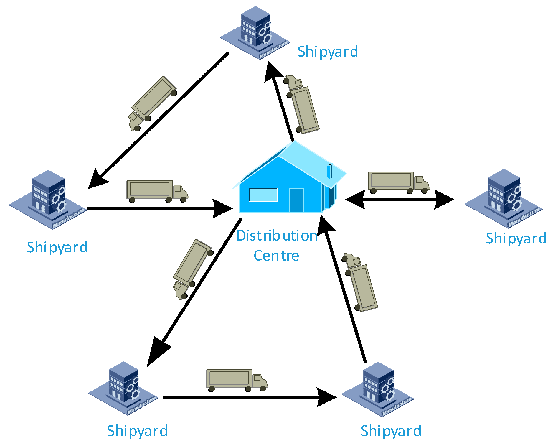
The vehicle routing problem between the steel distribution center and shipyard is shown in Figure 1, and can be described as follows: For a steel distribution center, there are a certain number of different types of vehicles, and at the same time, steel is transported to several designated shipyards. The quantity of steel that each shipyard needs to deliver and take is determined. Distribution centers assign vehicles to transport steel from distribution centers to shipyards according to the order requirements of different shipyards, and transport the goods that shipyards need to transport back to distribution centers from shipyards. Distribution centers need to consider comprehensively and make rational decisions on distribution vehicles, the distribution sequence, and distribution schemes. Under the constraints of satisfying the shipyard’s delivery demand and the maximum loading capacity of vehicles, the comprehensive cost, including depreciation cost, manpower cost, and carbon emissions are comprehensively considered to achieve the goal of lowest distribution cost.

The GVRSP-SPDTW problem studied in this paper can be defined as follows: There is a known steel distribution center which has a team of vehicles of the same type. Vehicles have a defined load capacity, fixed cost, carbon emissions, and other parameters. The distribution center serves N shipyards. The coordinates of each shipyard are known and the demand is known. Distribution vehicles load steel from the distribution center and deliver goods to N shipyards. Each shipyard is required to complete the delivery task using one vehicle. Each vehicle must start from the distribution center and return to the distribution center when the goods are delivered. The cost of each distribution vehicle consists of three parts: The fixed use cost of the vehicle, the cost of fuel and carbon emissions, and the driver’s salary. The optimization objective of this problem is to rationally allocate vehicles and arrange vehicle distribution routes to minimize the total cost, taking into account both vehicle operating costs (including fixed use costs and driver’s wages) and fuel and carbon emission costs.

3.2. Assumptions

Before further study, in order to facilitate the study of this problem and the establishment and solution of the model, the following assumptions are made:

(1)

There is only one distribution center and the location coordinates of the distribution center and the shipyards are known;

(2)

Two requirements for each shipyard are known;

(3)

The capacity of each vehicle can satisfy at least two requirements of a shipyard at the same time, and the vehicles in the distribution center can satisfy the distribution needs of all shipyards;

(4)

The load of each vehicle during transportation shall not exceed its maximum load;

(5)

Vehicles in distribution centers are of the same type and the maximum load is known;

(6)

Each vehicle leaves the distribution center and returns to the yard after serving all shipyards. Each shipyard is allowed to visit only once;

(7)

Vehicles can be loaded and unloaded immediately after arrival at the shipyard without waiting;

(8)

The time for shipyards to allow distribution centers to provide services is fixed;

(9)

The time spent in vehicle service is known, and the vehicle starts immediately after the shipyard completes the loading or unloading task.

3.3. Mathematical Model

Define a digraph as $G=\left(N,A\right)$, where $N=\left\{1,2,\dots ,n\right\}$ is a set of nodes. Node 1 represents the distribution center and $A=\left\{\left(i,j\right) i\ne j;i,j\in N\right\}$ represents the set of arcs between two nodes. $N_0=N|\left\{1\right\}$ represents the shipyard node. There are $K=\left\{1,2,\dots ,m\right\}$ vehicles of the same type in the yard and their maximum capacity is $Q$. Each arc $\left(i,j\right)$ represents the shortest distance between node $i$ and node $j$ and the distance between arc $\left(i,j\right)$ is represented by $d_{ij}$. Each shipyard has two requirements, $q_i$ means the weight of steel to be delivered to shipyard $i$ by the distribution center, $p_i$ means the weight of steel to be delivered to the distribution center by shipyard $i$, and shipyard $i$ allows the distribution center to distribute steel to shipyard $i$ during $\left[a_i,b_i\right]$ period. The arrival time of vehicle $k$ at shipyard $i$ is recorded as $t_{ik}$, and the service time of vehicle $k$ at shipyard $i$ is recorded as $t_{sik}$. Let the weight of the empty vehicle be $w_0$ and the load of the vehicle on Section $\left(i,j\right)$ be $w_{ij}$.

Therefore, the fuel and carbon emissions of the vehicle k traveling between the arc ends $\left(i,j\right)$ can be calculated according to the following formula [32]:

$$C_e{d}_{ij}\left[{\rho }_0+\alpha \left(Y_i^k+Z_i^k\right)\right]$$

(1)

where $C_e$ is the cost of fuel and carbon emissions per unit, $d_{ij}$ is the distance of arc section $\left(i,j\right)$, ${\rho }_0$ is the fuel consumption per unit distance to no-load vehicles, $\alpha$ is the additional fuel consumption per unit distance of goods loaded per unit weight, and $Y_i^k$ is the weight of the cargo on board from all the visited shipyards after vehicle $k$ arrives at shipyard $i$ to complete the loading and unloading task. $Z_i^k$ is the total amount of cargo needed to be delivered by all the shipyards to be visited after vehicle $k$ arrives at shipyard $i$ to complete the loading and unloading task.

Based on the above description and assumptions, the GVRSP-SPDTW problem is modeled as a MILP model. The parameters required in the MILP model are listed as follows:

• $F$: The objective function includes fixed use cost, fuel and carbon emission cost and driver’s salary.
• $N$: Set of nodes (including distribution centers).
• $N_0$: Shipyard assembly.
• $K$: Vehicle assembly.
• $d_{ij}$: Distance of arc segment $\left(i,j\right)$.
• $q_i$: The weight of steel that the distribution center needs to deliver to shipyard $i$.
• $p_i$: The weight of steel that shipyard $i$ needs to deliver to the distribution center.
• $\left[a_i,b_i\right]$: Delivery time window allowed by shipyard $i$.
• ${\rho }_0$: The amount of fuel consumed per unit distance for no-load vehicles.
• $\alpha$: Additional fuel consumption per unit distance for vehicles carrying goods per unit weight.
• $t_i^k$: The time when vehicle $k$ arrives at shipyard $i$.
• $t_{si}$: The loading and unloading service time of vehicle $k$ at shipyard $i$.
• $Trave{l}_{ij}^k$: The travel time of vehicle $k$ from node $i$ to node $j$.
• $Y_i^k$: The total weight of the cargo loaded on the vehicle $k$ after it arrives at the shipyard $i$ to complete the loading and unloading task from all the visited shipyards.
• $Z_i^k$: The total amount of cargo to be delivered by the shipyard after the vehicle $k$ arrives at the shipyard $i$ to complete the loading and unloading task.
• $C_v$: The fixed use cost of vehicles.
• $C_p$: Labor remuneration paid to drivers per unit time.
• $C_e$: Cost per unit of fuel and carbon emissions.

Decision variables:

• $x_{ij}^k$: When the vehicle $k$ serves the shipyard $i$ and then goes to the shipyard $i$ for loading and unloading service, $x_{ij}^k$ = 1; otherwise, $x_{ij}^k$ = 0.

In summary, the total costs considered in this model consists of three parts:

(1)

Fixed-use costs of vehicles:

$$C_v{\displaystyle \sum _{j\in N_0}{x}_{0j}};$$

(2)

(2)

Manpower expenditure of vehicles:

$$C_p{\displaystyle \sum _{k\in K}{\displaystyle \sum _{i\in N_0}{\displaystyle \sum _{j\in N_0}{d}_{ij}{x}_{ij}^k}}};$$

(3)

(3)

Fuel and carbon emission costs:

$$C_e{\displaystyle \sum _{k\in K}{\displaystyle \sum _{i\in N_0}{\displaystyle \sum _{j\in N_0}{d}_{ij}{x}_{ij}^k\left[{\rho }_0+\alpha \left(Y_i^k+Z_i^k\right)\right]}}}.$$

(4)

Therefore, the objective function can be expressed as:

$$F=C_v{\displaystyle \sum _{j\in N_0}{x}_{0j}}+C_p{\displaystyle \sum _{k\in K}{\displaystyle \sum _{i\in N_0}{\displaystyle \sum _{j\in N_0}{d}_{ij}{x}_{ij}^k}}}+C_e{\displaystyle \sum _{k\in K}{\displaystyle \sum _{i\in N_0}{\displaystyle \sum _{j\in N_0}{d}_{ij}{x}_{ij}^k\left[{\rho }_0+\alpha \left(Y_i^k+Z_i^k\right)\right]}}}+{\displaystyle \sum _{i\in N_0}{w}_i}{T}_{late}^i.$$

(5)

The constraints are:

$${\displaystyle \sum _{j\in N_0}{x}_{0j}^k}=1 \forall k\in K$$

(6)

$${\displaystyle \sum _{k\in K}{x}_{ij}^k=1 \forall i\in N},\forall j\in N$$

(7)

$${\displaystyle \sum _{k\in K}{\displaystyle \sum _{j\in N}{x}_{ij}^k}=1 \forall i\in N_0}$$

(8)

$$Y_0^k=0 \forall k\in K$$

(9)

$$Y_i^k={\displaystyle \sum _{l\in N}\left(Y_l^k+p_i\right)} x_{li}^k \forall k\in K$$

(10)

$$Z_0^k={\displaystyle \sum _{i\in N}{\displaystyle \sum _{j\in N_0}{q}_j}}{x}_{ij}^k \forall k\in K$$

(11)

$$Z_i^k={\displaystyle \sum _{l\in N}\left(Z_l^k-q_i\right)}{x}_{li}^k \forall k\in K$$

(12)

$$Y_i^k+Z_i^k\le Q \forall k\in K,\forall i\in N$$

(13)

$${\displaystyle \sum _{i\in N}{x}_{ij}^k}={\displaystyle \sum _{m\in N}{x}_{jm}^k} \forall j\in N_0$$

(14)

$$t_j^k={\displaystyle \sum _{j\in N}\left(t_i^k+t_{si}^k+Trave{l}_{ij}^k\right)x_{ij}^k} \forall k\in K$$

(15)

$$a_j\le t_j^k\le b_j-t_{si}.$$

(16)

Equations (6)–(8) guarantee that each shipyard can only be served once. Equation (9) indicates that when the vehicle $k$ starts from the distribution center, the weight of the cargo on board from all the visited shipyards is zero. Equation (10) denotes the weight of cargo obtained from all visited shipyards on board after vehicle $k$ arrives at shipyard $i$ to complete the loading and unloading task. Equation (11) denotes the total amount of cargo to be distributed by all subsequent shipyards on board when vehicle $k$ departs from the distribution center. Equation (12) denotes the total amount of cargo to be delivered by all subsequent shipyards to be visited after the arrival of vehicle $k$ at shipyard $i$, and Equation (13) denotes that the total amount of cargo carried by each vehicle cannot exceed the maximum capacity of the vehicle. Equation (14) guarantees that the same vehicle arrives and leaves each shipyard. Equation (15) indicates the time when the vehicle $k$ arrives at the shipyard. Equation (16) ensures that the arrival time of vehicle $k$ at the shipyard is not earlier than the earliest time window required by the shipyard, and that the arrival time at the shipyard and the completion of unloading are not later than the latest time window required by the shipyard.

4. Improved Intelligent Water Drop Algorithms

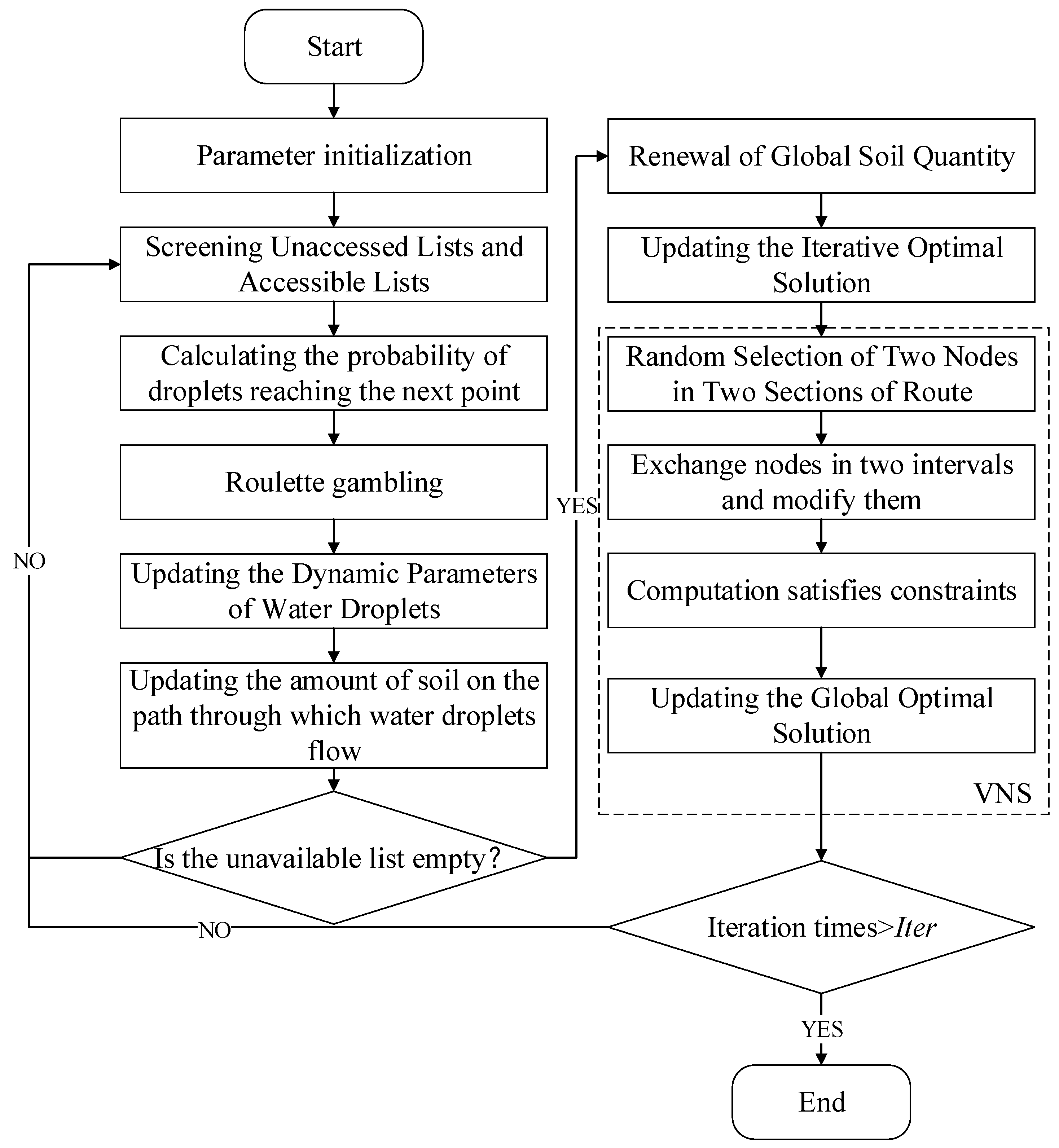
The intelligent water drop algorithm is an algorithm that simulates the movement of water drops in nature and finds the best path. Each water drop simulates the movement of a car. Each drop starts from the distribution center, chooses the next accessible node from the unavailable list, and updates the weight of the goods carried by the vehicle. When the weight of the water drops exceeds the vehicle load or all accessible nodes are visited, the water drops return to the distribution center, which constitutes a completed vehicle route. The next intelligent water drop starts to run until all nodes are visited and completed in an iteration. Traditional intelligent water drop algorithms tend to converge slowly and often fall into a local optimum. In order to avoid this situation, an improved Intelligent Water Drop (IIWD) algorithm was designed. Elite strategy and variable neighborhood search mechanisms were added to effectively ensure that the algorithm jumps out of local optimum and avoids falling into a premature optimum.

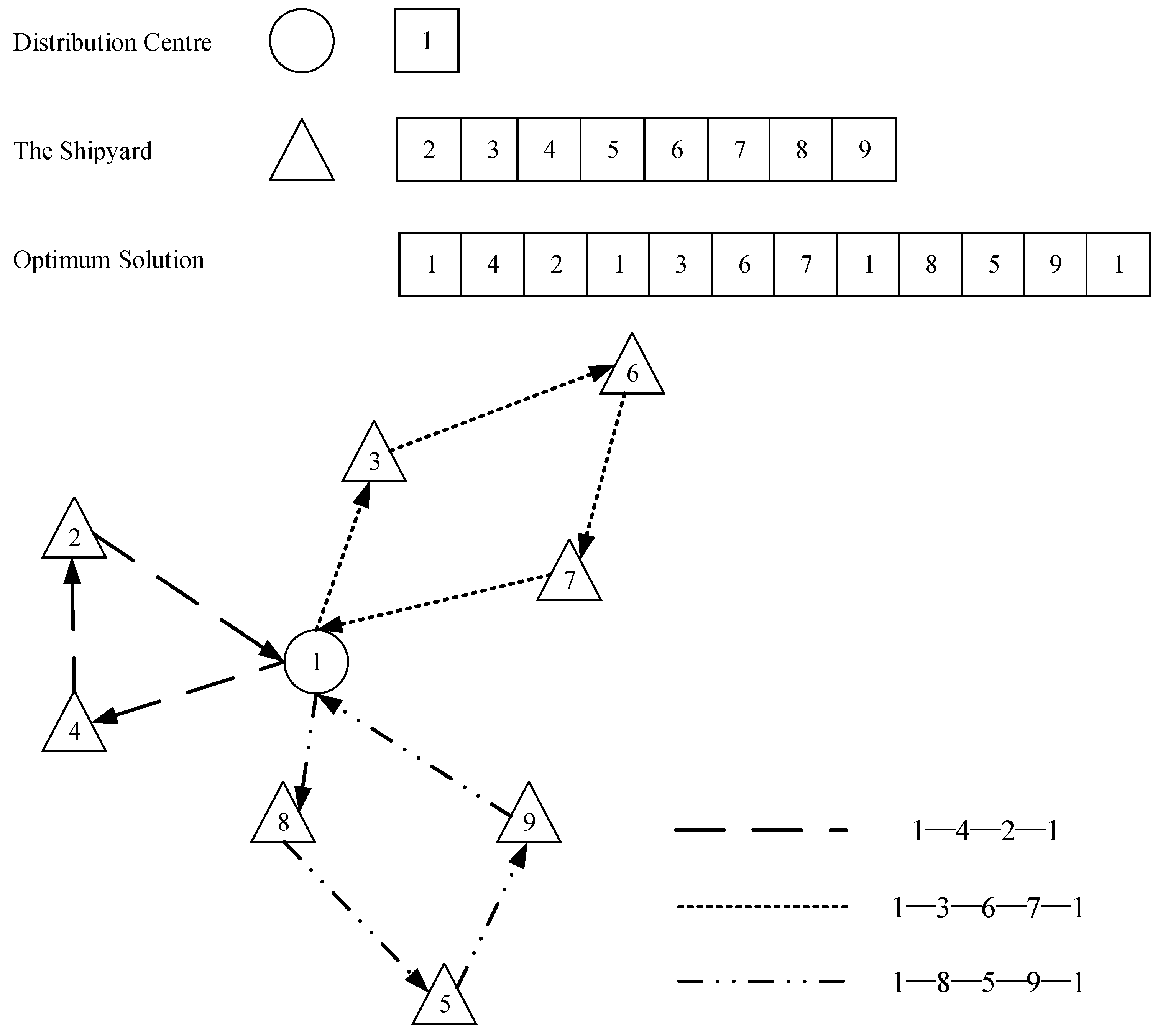
A water drop starts from distribution center 1, travels through various demand points along different paths, and finally returns to the distribution center to form a complete flow path of water drops (water drops in the path can pass through distribution center 1 many times, but each demand point can only pass once). The complete flow path of each water drop corresponds to a solution of the problem. If the complete flow path of a water drop is 1→4→2→1→3→6→7→1→8→5→9→1, the distribution path of three vehicles is 1→4→2→1, 1→3→6→7→1, 1→8→5→9→1. A concrete example is shown in Figure 2.

The specific design of the improved intelligent water drop algorithm is as follows:

Step 1: Parameter initialization. Static variables include: drop number N, initial velocity Initvel, iteration maximum number Iter, drop velocity update parameters $a_v$, $b_v$, $c_v$, soil quantity update parameters $a_s$, $b_s$, $c_s$, local and global soil renewal coefficients ${\rho }_0$ and ${\rho }_{IWD}$, initial state path soil amount Initsoil, and other static variables needed for solving mathematical models. The traditional intelligent water drop algorithm gives the same initial velocity and the same initial path soil amount to each water drop, but it is well known that the choice of initial solution will have a certain impact on the quality of the solution. Therefore, the initial velocity of each water drop and the amount of soil along the path are generated randomly to ensure diversity of the initial solution and improve the quality of the solution.

Step 2: The initial point is the distribution center node. According to the delivery time window and delivery volume requirements of other nodes, the required nodes are selected from the list of visiting nodes (UnvisitNode) and stored in the list of accessible nodes (FitVisit).

Step 3: Calculating the accessibility probability $p_i$ of each node in the list of accessible nodes (FitVisit) and choosing the next serviceable node by roulette can improve the global search ability and avoid falling into local optimum:

$$p_i=\frac{f\left(Soi{l}_{i,j}\right)}{{\displaystyle \sum _{k\in FitVisit}f\left(Soi{l}_{i,k}\right)}}$$

(17)

$$f\left(Soi{l}_{i,j}\right)=\frac{1}{\epsilon +g\left(Soi{l}_{i,j}\right)}$$

(18)

$$g\left(Soi{l}_{i,j}\right)=\{\begin{array}{l}Soi{l}_{i,j}; if \min \left(Soi{l}_{i,k}\right)\ge 0\hfill \\ Soi{l}_{i,j}-\min \left(Soi{l}_{i,k}\right); else\hfill \end{array}.$$

(19)

In this formula, the constant $\epsilon$ is 0.01, which ensures that the denominator of function $f\left(Soi{l}_{i,j}\right)$ is not zero, function $g\left(Soi{l}_{i,j}\right)$ ensures that the amount of soil is positive, and $\min \left(Soi{l}_{i,k}\right)$ is the minimum amount of soil on the path from the current node to all serviceable nodes.

Step 4: Update the dynamic parameters of intelligent water drops. Update the flow velocity $Ve{l}_{IWD}\left(t\right)$ of intelligent water drops from the current node to the next selected node according to the following formula:

$$Ve{l}_{IWD}\left(t\right)=Ve{l}_{IWD}\left(t-1\right)+\frac{a_v}{b_v+c_v\times Soi{l}_{i,j}^2}.$$

(20)

where $a_v$, $b_v$, and $c_v$ are the update parameters of drop velocity, and $Soi{l}_{i,j}^{}$ is the path soil amount from the current node to the selected next node.

Similarly, calculating the time $T_{i,j}$ needed for intelligent water drops to flow to the target point, and the increment $\Delta Soi{l}_{i,j}$ of soil carried by water drops, can be done as shown below:

$$T_{i,j}=\frac{d_{i,j}}{\max \left({\epsilon }_v,Ve{l}_{IWD}\left(t\right)\right)}$$

(21)

$$\Delta Soi{l}_{i,j}=\frac{a_s}{b_s+c_s\times T_{i,j}^2}$$

(22)

where $d_{i,j}$ is the distance from the current node to the next selected node, constant ${\epsilon }_v$ ensures that the denominator is not zero, and $a_s$, $b_s$ and $c_s$ are the updated parameters of soil increment $\Delta Soi{l}_{i,j}$.

Step 5: Update the amount of soil $Soi{l}_{i,j}$ on the path through which water drops flow. In the process of water drop flow, the soil content in the path changes dynamically with the flow of water drops. When the soil content in one path is much higher than that in other paths, the algorithm will converge ahead of time and cannot get a better solution. Similarly, when the soil content in a certain path is less, the convergence speed of the algorithm will be slowed down. In order to prevent the slow/premature convergence of the algorithm, referring to the bounded soil renewal model proposed by Niu et al. [33], this paper sets the maximum and minimum limits on the amount of soil in each path, slows down the fast convergence when the amount of soil is too large, and improves the convergence speed when the amount of soil is small. Therefore, in the improved intelligent water drop algorithm, the formulas for calculating the amount of soil flowing through the path and the amount of soil carried by the water drop are as follows:

$$\stackrel{-}{\Delta }Soi{l}_{i,j}=\{\begin{array}{l}\Delta Soi{l}_{i,j}^{\min }; if \Delta Soi{l}_{i,j}<\Delta Soi{l}_{i,j}^{\min }\hfill \\ \Delta Soi{l}_{i,j}^{\max };if \Delta Soi{l}_{i,j}> \Delta Soi{l}_{i,j}^{\max }\hfill \\ \Delta Soi{l}_{i,j}; else\hfill \end{array}$$

(23)

$$Soi{l}_{i,j}^{}\left(t\right)=\left(1-{\rho }_0\right)Soi{l}_{i,j}^{}\left(t-1\right)-{\rho }_0\stackrel{-}{\Delta }Soi{l}_{i,j}$$

(24)

$$Soi{l}_{i,j}^{IWD}\left(t\right)=Soi{l}_{i,j}^{IWD}\left(t-1\right)+\stackrel{-}{\Delta }Soi{l}_{i,j}$$

(25)

where $\Delta Soi{l}_{i,j}^{\min }$ and $\Delta Soi{l}_{i,j}^{\max }$ are respectively the minimum and maximum limit of the increment of soil carried by water drops, $Soi{l}_{i,j}^{}\left(t\right)$ is the amount of soil carried by water drops on the path, $Soi{l}_{i,j}^{IWD}\left(t\right)$ is the amount of soil carried by water drops, and ${\rho }_0$ is the local renewal coefficient, which has a value of 0.9.

Step 6: If the selected target node is the distribution center, the distribution vehicle returns to the distribution center. Otherwise, update the visited list and the unavailable list, and turn to step 2 until the unavailable list is empty, indicating that all the required nodes have been served, and each water drop forms a complete access path. By calculating the value of the objective function, the minimum feasible solution of the objective function value is determined by comparison, which is the optimal solution $S^{IB}$ of this iteration.

Step 7: Global soil quantity renewal. The soil amount on the path corresponding to the optimal solution obtained by this iteration is updated:

$$Soi{l}_{i,j}^{}=\left(1+{\rho }_{IWD}\right)Soi{l}_{i,j}^{}-\frac{{\rho }_{IWD}Soi{l}_k^{IWD}}{n-1}$$

(26)

where ${\rho }_{IWD}$ is the global soil quantity renewal coefficient, $Soi{l}_k^{IWD}$ is the soil quantity carried by the water drops corresponding to the k-th iteration optimal solution, and n is the number of nodes on the path corresponding to the iteration optimal solution.

Step 8: Update the global optimal solution:

$$S^{TB}=\{\begin{array}{l}{S}^{TB}; if f\left(S^{TB}\right)<f\left(S^{IB}\right)\hfill \\ S^{IB}; else\hfill \end{array}.$$

(27)

Step 9: The global optimal solution obtained by the improved intelligent water drop algorithm is further optimized using the variable neighborhood search algorithm. By using the vibration method and introducing the interference factor into the algorithm, a new path order is obtained by resetting and inserting the location of the sorting points in the neighborhood of the optimal path, and the distribution time of the sorting points after insertion and the constraint satisfaction of the vehicle load are checked. Finally, a new path satisfying the constraint is obtained. To a certain extent, the intelligent water drop algorithm can jump out of the local optimum and accelerate the convergence speed of the algorithm. The pseudo code of the variable neighborhood algorithm is given below.

Algorithm 1 Procedure Variable Neighborhood Search

Begin

1: Initialize the set of neighborhood structure Nk, k=1,…,kmax;

2: Generate the initial solution S;

3: repeat

4: k ← 1;

5: repeat

6: ShakeMethod(S, S’);

7: ImprovementMethod(S’, S”);

8: if J (S”) ≥ J (S) then{

9: S ← S”;

10: k ← 1;

11: }

12: else

13: k ← k + 1;

14: until (k = kmax)

15: until (StoppingCriterion)

End

Step 10: Update the iteration coefficient. Return to step 2 until the iteration is completed, and output the optimal solution.

The specific algorithm design flow is shown in Figure 3.

5. Computational Experiments

In this section, the performance of proposed methods is evaluated by 100 randomly generated instances, including small, medium, and large-size ones. In this paper, the classical Solomon example [34] of the vehicle routing problem with time windows is improved, and the parameters of pick-up are added. The GA algorithm, traditional intelligent water droplet algorithm, and improved intelligent water droplet algorithm are compared and calculated. The results are shown in

Table 1. Verification results.

Problem Group	GA	IDW	IIDW
	Cost	Cost	Cost
R101	57,030	56,140	55,230
R102	56,180	56,150	54,330
R103	65,860	63,230	57,212
R104	61,471	59,840	57,178
R105	62,480	67,270	61,847
R106	60,080	58,840	57,106
R107	59,020	58,120	57,955
R108	57,732	58,400	58,048
R109	59,310	57,650	56,759
R110	54,700	58,280	57,486
R111	57,390	57,750	56,267
R112	56,180	57,470	57,321

Bold numbers: represent the best values in each line.

. All algorithms were coded in MATLAB R2014b. All computational experiments were conducted on a PC with a 3.60 GHz processor and 8.00 GB RAM under the Windows 10 operating system. For the augmented e-constraint method, CPLEX 12.6 was used to solve single-objective problems. The computation time for each single-objective optimization and the total computational time were limited to within 7200 and 36,000 s, respectively.

From Table 1, it can be seen that the improved intelligent water drop algorithm can obtain better solutions in most cases, so it can be explained that the intelligent water drop algorithm has better applicability for such problems.

To verify the validity of the IIWD algorithm proposed in this paper, the methods of Wang and Chen were used to calculate an example [35] for simultaneous delivery and delivery with time windows. Specific data are shown in

Table 2. Relevant data.

Distribution Point	X Coordinates	Y Coordinates	Requirement	Quantity of Pick-Up	Service Time	Time Window
1	0	40	50	0	0	0
2	4	20	80	40	20	30
3	20	42	15	10	10	0
4	22	40	15	40	30	0
5	29	90	35	10	20	0
6	31	88	35	20	30	0
7	33	85	25	10	10	0
8	36	65	85	40	30	0
9	38	62	80	30	40	20
10	46	18	80	10	10	0
11	53	20	50	5	5	20
12	60	15	60	17	5	0
13	62	65	35	3	21	12
14	66	41	37	16	18	0
15	70	35	69	23	4	0
16	76	60	12	31	11	40
17	77	23	3	7	5	15
18	78	8	56	27	5	0
19	80	47	47	13	10	0
20	81	49	58	10	16	0
21	87	12	24	13	6	30
22	88	24	58	19	32	0
23	92	53	43	14	12	14
24	93	61	52	3	7	40
25	95	56	37	6	3	0
26	99	26	35	15	5	20

(serial number 1 indicates distribution center point), and the initialization parameters are shown in

Table 3. Initialization parameters.

Q	Vehicle rated load	49 t	$a_s$	Renewal parameters of soil and water drops	1000
$v_k$	Average Vehicle Speed	40 km/t	$b_s$	Renewal parameters of soil and water drops	0.01
$C_v$	Fixed-use costs of vehicles	200/one	$c_s$	Renewal parameters of soil and water drops	1
$C_p$	Unit Transportation Cost per Vehicle	10/km	Initsoil	Initial path amount of soil	1000
$N_{IWD}$	Number of drops	20	Initvel	Initial drop velocity	100
$a_v$	Drop Velocity Updating Parameters	1	${\rho }_0$	Local soil renewal parameters	0.9
$b_v$	Drop Velocity Updating Parameters	0.01	${\rho }_{IWD}$	Global soil renewal parameters	0.8
$c_v$	Drop Velocity Updating Parameters	1	Iter	Maximum number of iterations	100
${\rho }_0$	Fuel consumption per unit distance for no-load vehicles	2	$\alpha$	Additional fuel consumption per unit distance for vehicles carrying goods per unit weight	0.8

.

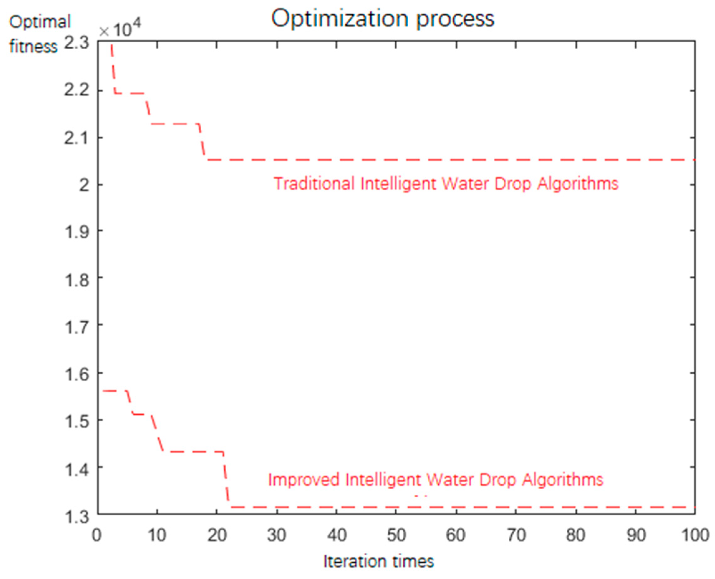
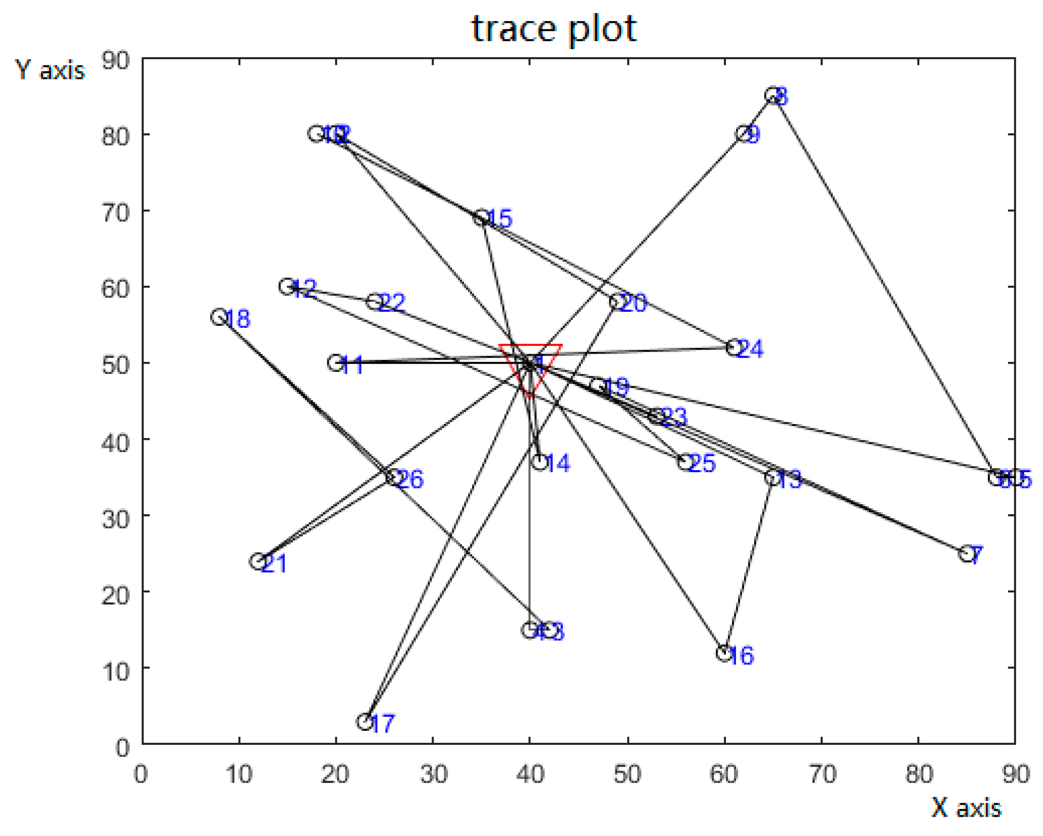
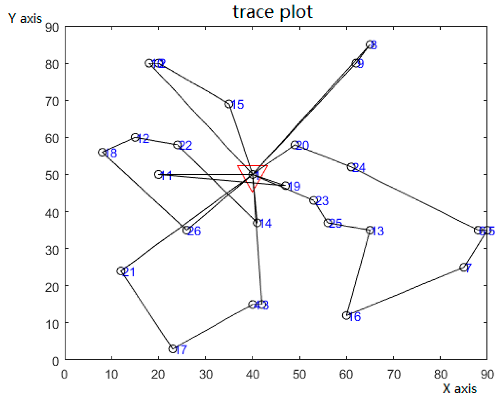
The simulation results show that the improved intelligent water drop algorithm has faster convergence speed and higher efficiency than the traditional intelligent water drop algorithm when solving the GVRSP-SPDTW problem, as shown in Figure 4. This is because the improved algorithm can reset and insert some nodes of the better solution after iteration, which can overcome the problem of long search time of the traditional intelligent water drop algorithm and effectively avoid the shortcoming of falling into local optimum in the search process. When the total number of iterations is 23, the optimal solution of the model can be obtained. At this time, six vehicles are allocated. The specific allocation scheme and vehicle routing are shown in

Table 4. Optimal vehicle routing and total cost (improved intelligent water drop algorithms).

Vehicle Number	Route	Total Cost	Total Distance
1	14-22-12-18-26	13,155	655.66
2	10-2-15
3	20-24-6-5-7-16-13-25-23
4	11-19
5	9-8
6	21-17-4-3

. The Figure 5 and Figure 6 are diagrams of the optimal routes of the two algorithms.

Based on the above, a steel distribution center in Shanghai and 18 shipyards around it are taken as an example to analyze. Their locations are sorted out by a Baidu Map, and customer requirements and acceptable time windows are known. The IWD and IIWD algorithm designed in this paper are used to solve the problem. The distribution center uses six-axle trucks for distribution service. According to the national truck load standard, the rated load of six-axle trucks is 49 tons. Specific data are shown in

Table 5. Relevant data of distribution center and shipyard.

Distribution Point	X Coordinates	Y Coordinates	Requirement	Quantity of Pick-Up	Service Time	Time Window
1	18.7	15.29	0	0	0	(0,40)
2	16.47	8.45	6	3.6	1.8	(5,20)
3	20.07	10.14	5	2	1	(4,15)
4	19.39	13.37	11	4.6	2.3	(1,20)
5	25.27	14.24	6	3.6	1.8	(2,20)
6	22	10.04	3	2.4	1.2	(5,15)
7	25.47	17.02	8	4.8	2.4	(2,18)
8	15.79	15.1	5	3	1.5	(1,24)
9	16.6	12.38	6	3.6	1.8	(3,27)
10	14.05	18.12	4	2.4	1.2	(1,20)
11	17.53	17.38	5	3	1.5	(2,16)
12	23.52	13.45	7	4.2	2.1	(2,20)
13	19.41	18.13	6	3.6	1.8	(2,10)
14	22.11	12.51	10	4	2	(3,25)
15	11.25	11.04	9	5.4	2.7	(2,28)
16	14.17	9.76	4	2.6	1.3	(3,24)
17	24	19.89	7	2.4	1.2	(2,20)
18	12.21	14.5	8	3	1.5	(1,23)

(serial number 1 indicates distribution center point), and initialization parameters are the same as seen in Table 3.

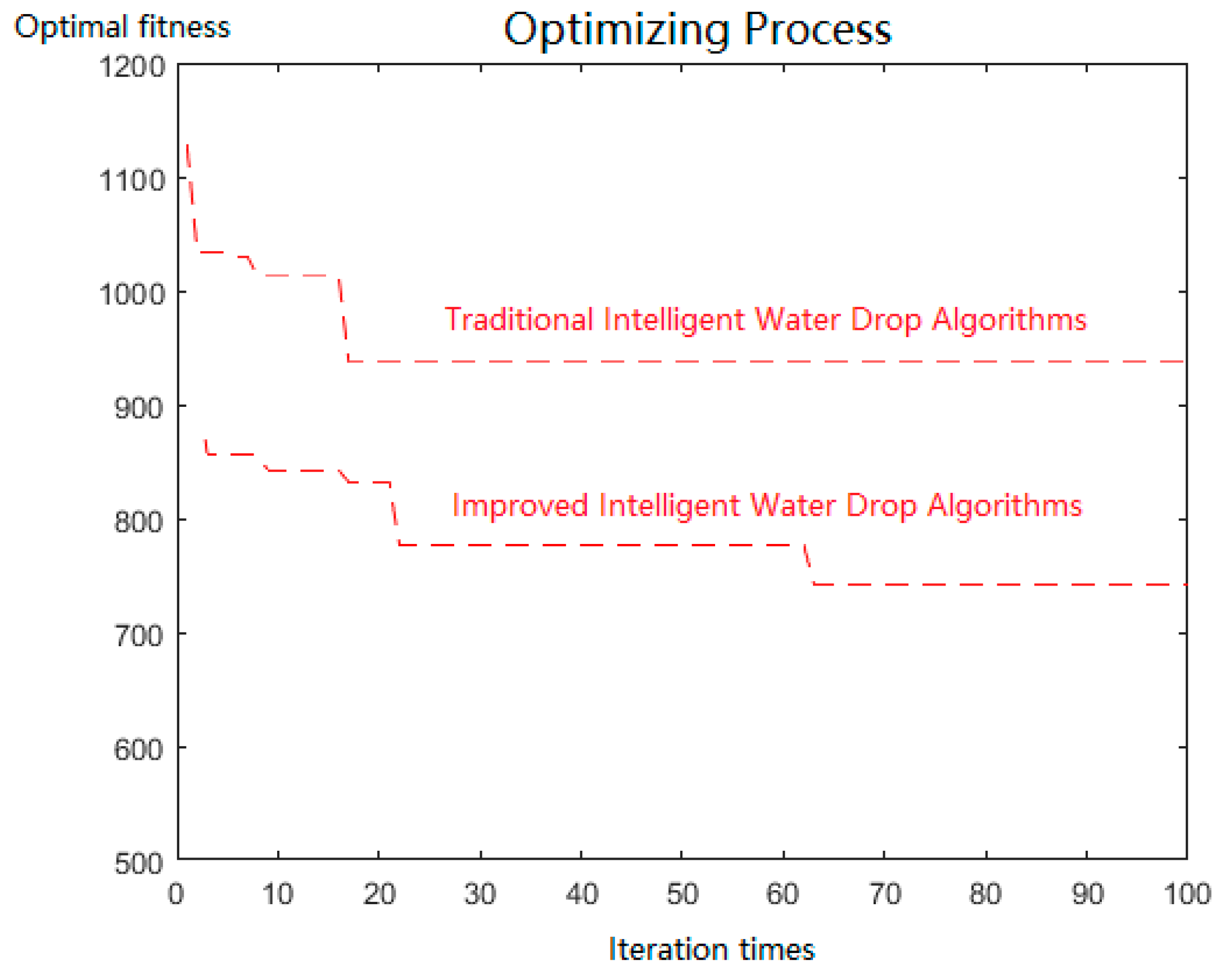
The example was programmed using MATLAB2016 software. The running environment is 8000 memory and a Windows 8 operating system. The specific running iteration process is shown in Figure 7.

6. Discussion

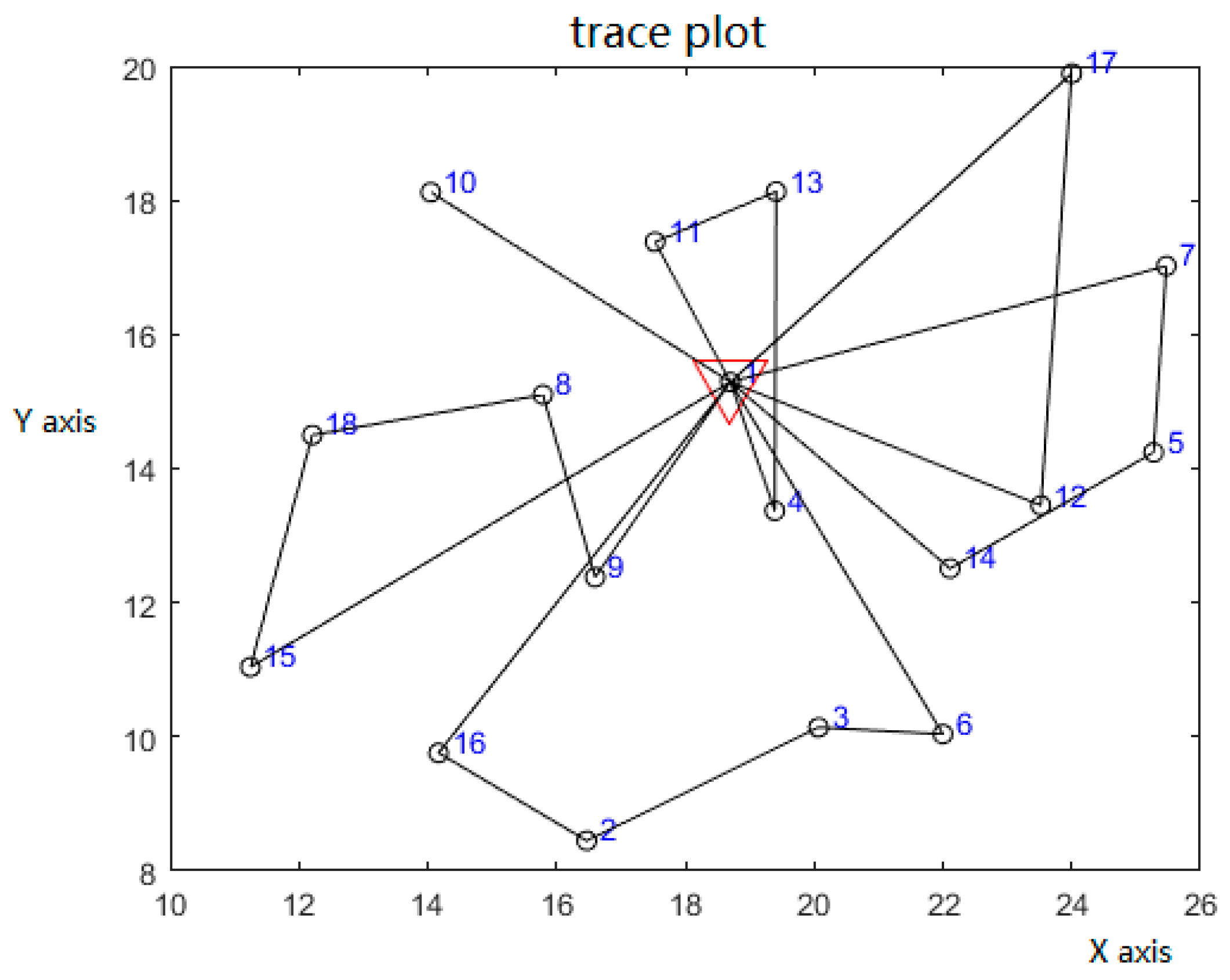
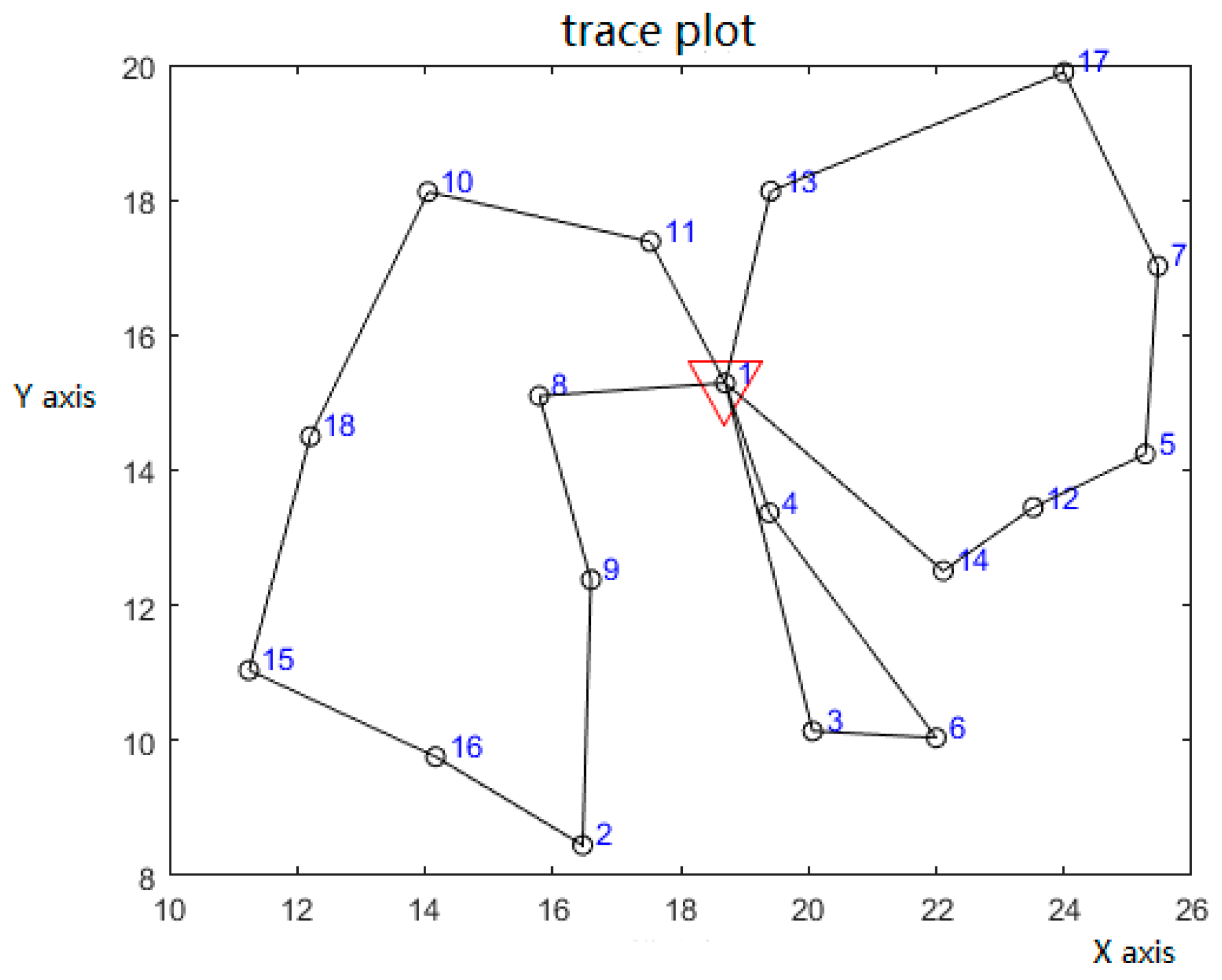
As can be seen from Figure 7, when the improved intelligent water drop algorithm iterates 61 times, the optimal solution of the model can be obtained. At this moment, there are three vehicles for distribution. The specific allocation scheme and vehicle routing are shown in

Table 6. Vehicle optimal routing and total cost (traditional intelligent water drop algorithms).

Vehicle Number	Route	Total Cost (¥)	Total Distance (km)
1	15-18-8-9	937	102.65
2	14-5-7
3	12-17
4	6-3-2-16
5	10
6	11-13-4

and

Table 7. Optimal vehicle routing and total cost (improved intelligent water drop algorithms).

Vehicle Number	Route	Total Cost (¥)	Total Distance (km)
1	11-10-18-15-16-2-9-8	741.98	91.297
2	14-12-5-7-17-13
3	4-6-3

. From Table 6 and Table 7, it can be seen that the total cost after improving the optimization results of the intelligent water drop algorithm is ¥195.02 less than that of traditional intelligent water drop algorithm, which can save about 20% of the cost. The improved intelligent water drop algorithm runs 11.353 km less than the traditional intelligent water drop algorithm. The number of vehicles used in the improved intelligent water drop algorithm is only half that of the traditional intelligent water drop algorithm. In conclusion, when solving the GVRSP-SPDTW problem, the improved intelligent water drop algorithm has faster convergence speed and higher efficiency than the traditional intelligent water drop algorithm. The Figure 8 and Figure 9 are diagrams of the optimal routes of the two algorithms.

7. Conclusions

In order to solve the vehicle routing and scheduling problem of a ship steel distribution center under the green shipbuilding model, based on the conventional vehicle routing problem model, the amount of carbon dioxide emitted by vehicles is set as one of the optimization objectives. A mathematical model of total cost optimization is established, which aims at the optimization of vehicle depreciation cost, manpower cost, and carbon emissions. A green vehicle routing and scheduling optimization method based on IIWD is proposed. By comparing with GA and the traditional IWD algorithm, it was proven that the green vehicle routing and scheduling optimization method based on IIWD proposed in this paper can greatly reduce the total cost of vehicle distribution, and then reduce the carbon emissions in the process of vehicle distribution. While ensuring the progress of ship construction, this algorithm meets the requirements of green environmental protection, thus realizing a real part of green shipbuilding. The green vehicle routing and scheduling optimization method based on IIWD proposed in this paper has certain practical value and theoretical significance. In a follow-up study, multi-type vehicles and dynamic time windows in multi-distribution centers are considered in the mathematical model, and corresponding algorithms are designed for the model to further improve the practicability of the study.

References

- Demartini, M.; Orlandi, I.; Tonelli, F.; Anguitta, D. A Manufacturing Value Modeling Methodology (MVMM): A Value Mapping and Assessment Framework for Sustainable Manufacturing. In Proceedings of the International Conference on Sustainable Design & Manufacturing, Bologna, Italy, 26–28 April 2017; Springer: Cham, Switzerland, 1842. [Google Scholar]
- Tonelli, F.; Evans, S.; Taticchi, P. Industrial Sustainability: Challenges, perspectives, actions. Int. J. Bus. Innov. Res. 2013, 7, 143–163. [Google Scholar] [CrossRef]
- Wang, J.; Zhang, H. Research status and Prospect of green manufacturing technology based on product life cycle. Comput. Integr. Manuf. Syst. 1999, 4, 1–8. [Google Scholar]
- Zhao, Z. On Green Shipbuilding Technical System; China Shipbuilding: Beijing China, 2009; Volume 49, pp. 36–40. [Google Scholar]
- Tan, N. Development Trend of China’s Shipbuilding Industry and Demand for Steel. Shipbuild. Mater. Mark. 2008, 3, 25–29. [Google Scholar]
- Shen, W. A Brief Discussion on the Present Situation and Development of Ship Steel Distribution Center. Ship Mater. Mark. 2012, 6, 37–39. [Google Scholar]
- Sanchez Vicente, A.; Pastorello, C.; Foltescu, V.L. The contribution of transport to air quality. In TERM 2012: Transport Indicators Tracking Progress towards Environmental Targets in Europe; Publication of European Environment Agency, 2012; Available online: https://www.eea.europa.eu/ (accessed on 1 August 2019).
- Li, L.; Xing, J. Research on Low Carbon Logistics Development in China under Low Carbon Economic Trend. Bus. Econ. Res. 2011, 31, 24–25. [Google Scholar]
- Dantzig, G.B.; Ramser, J.H. The Truck Dispatching Problem. Manag. Sci. 1959, 6, 80–91. [Google Scholar] [CrossRef]
- Min, H. The multiple vehicle routing problem with simultaneous delivery and pickup. Transp. Res. Part A Gen. 1989, 23, 377–386. [Google Scholar] [CrossRef]
- Gendreau, M.; Laporte, G.; Séguin, R. Stochastic vehicle routing. Eur. J. Oper. Res. 1996, 88, 3–12. [Google Scholar] [CrossRef]
- Teodorovic, D.; Pavkovic, G. A simulated annealing technique approach to the vehicle routing problem in the case of stochastic demand. Transp. Plan. Technol. 1992, 16, 261–273. [Google Scholar] [CrossRef]
- Xiao, Y.; Zhao, Q.; Kaku, I.; Xu, Y. Development of a fuel consumption optimization model for the capacitated vehicle routing problem. Comput. Oper. Res. 2012, 39, 1419–1431. [Google Scholar] [CrossRef]
- Xiao, Y.; Konak, A. A genetic algorithm with exact dynamic programming for the green vehicle routing & scheduling problem. J. Clean. Prod. 2003, 30, 787–800. [Google Scholar]
- Jabali, O.; Woensel, T.V.; De Kok, A.G. Analysis of Travel Times and CO2 Emissions in Time-Dependent Vehicle Routing. Prod. Oper. Manag. 2012, 21, 1060–1074. [Google Scholar] [CrossRef]
- Urquhart, N.; Scott, C.; Hart, E. Using an Evolutionary Algorithm to Discover Low CO2 Tours within a Travelling Salesman Problem. Lect. Notes Comput. Sci. 2010, 6025, 421–430. [Google Scholar]
- Kwon, Y.J.; Choi, Y.J.; Lee, D.H. Heterogeneous fixed fleet vehicle routing considering carbon emission. Transp. Res. Part D Transp. Environ. 2013, 23, 81–89. [Google Scholar] [CrossRef]
- Huang, Y.; Shi, C.; Zhao, L.; Van Woensel, T. A study on carbon reduction in the vehicle routing problem with simultaneous pickups and deliveries. In Proceedings of the IEEE International Conference on Service Operations & Logistics, Suzhou, China, 8–10 July 2012; IEEE: Piscataway, NJ, USA, 1963. [Google Scholar]
- Suzuki, Y. A new truck-routing approach for reducing fuel consumption and pollutants emission. Transp. Res. Part D Transp. Environ. 2011, 16, 73–77. [Google Scholar] [CrossRef]
- Zhang, S.; Lee, C.K.M.; Choy, K.L.; Ho, W.; Ip, W.H. Design and development of a hybrid artificial bee colony algorithm for the environmental vehicle routing problem. Transp. Res. Part D Transp. Environ. 2014, 31, 85–99. [Google Scholar] [CrossRef] [Green Version]
- Pei-Ying, Y. Minimizing Carbon Emissions for Vehicle Routing and Scheduling in Picking up and Delivering Customers to Airport Service. Acta Autom. Sin. 2013, 39, 424–432. [Google Scholar] [CrossRef]
- Bauer, J.; Bektaş, T.; Crainic, T.G. Minimizing greenhouse gas emissions in intermodal freight transport: An application to rail service design. J. Oper. Res. Soc. 2010, 61, 530–542. [Google Scholar] [CrossRef]
- Konak, A.; Konak, A. A Simulating Annealing Algorithm to Solve the Green Vehicle Routing & Scheduling Problem with Hierarchical Objectives and Weighted Tardiness; Elsevier Science Publishers B.V.: Amsterdam, The Netherlands, 2015. [Google Scholar]
- Xiao, Y.; Konak, A. The heterogeneous green vehicle routing and scheduling problem with time-varying traffic congestion. Transp. Res. Part E Logist. Transp. Rev. 2016, 88, 146–166. [Google Scholar] [CrossRef]
- Shahhosseini, H. Problem solving by intelligent water drops. In Proceedings of the IEEE Congress on Evolutionary Computation, Singapore, 25–28 September 2007; IEEE: Piscataway, NJ, USA, 1963. [Google Scholar]
- Alijla, B.O.; Wong, L.P.; Lim, C.P.; Khader, A.T.; Al-Betar, M.A. A modified Intelligent Water Drops algorithm and its application to optimization problems. Expert Syst. Appl. 2014, 41, 6555–6569. [Google Scholar] [CrossRef]
- Shah-Hosseini, H. Intelligent water drops algorithm: A new optimization method for solving the multiple knapsack problem. Int. J. Intell. Comput. Cybern. 2008, 1, 193–212. [Google Scholar] [CrossRef]
- Booyavi, Z.; Teymourian, E.; Komaki, G.M.; Sheikh, S. An improved optimization method based on the intelligent water drops algorithm for the vehicle routing problem. In Proceedings of the IEEE Computational Intelligence in Production & Logistics Systems, 7–10 December 2015; IEEE: Piscataway, NJ, USA, 1963. [Google Scholar]
- Niu, S.H.; Ong, S.K.; Nee, A.Y.C. An improved Intelligent Water Drops algorithm for achieving optimal job-shop scheduling solutions. Int. J. Prod. Res. 2012, 50, 14. [Google Scholar] [CrossRef]
- Kamkar, I.; Akbarzadeh-T, M.R.; Yaghoobi, M. Intelligent water drops a new optimization algorithm for solving the Vehicle Routing Problem. In Proceedings of the IEEE International Conference on Systems Man & Cybernetics, Istanbul, Turkey, 10–13 October 2010; IEEE: Piscataway, NJ, USA, 1963. [Google Scholar]
- Teymourian, E.; Kayvanfar, V.; Komaki, G.M.; Zandieh, M. Enhanced intelligent water drops and cuckoo search algorithms for solving the capacitated vehicle routing problem. Inf. Sci. 2016, 334–335, 354–378. [Google Scholar] [CrossRef]
- Barth, M.; Boriboonsomsin, K. Real-World CO2 Impacts of Traffic Congestion. In Proceedings of the 87th Transportation Research Board Annual Conference, Washington, DC, USA, 13–17 January 2008. [Google Scholar]
- Niu, S.H.; Ong, S.K.; Nee, A.Y.C. Improved Intelligent Water Drops Optimization Algorithm for Achieving Single and Multiple Objective Job Shop Scheduling Solutions. 2014, pp. 3451–3474. Available online: https://0-link-springer-com.brum.beds.ac.uk/referenceworkentry/10.1007%2F978-1-4471-4670-4_25#citeas URL (accessed on 1 August 2019).
- Wicker, S.B.; Bhargava, V.K. Reed-Solomon Codes and Their Applications; John Wiley & Sons: Hoboken, NJ, USA, 1999. [Google Scholar]
- Wang, H.F.; Chen, Y.Y. A genetic algorithm for the simultaneous delivery and pickup problems with time window. Comput. Ind. Eng. 2012, 62, 84–95. [Google Scholar] [CrossRef]
Figure 1.
Schematic diagram of vehicle routing problem between steel the distribution center and shipyard.
Figure 2.
An example of optimal solution coding.
Figure 3.
Flowchart of algorithm.
Figure 4.
Iterative contrast graph of algorithms.
Figure 5.
Road Map of Traditional Intelligent Water Drop Algorithms.
Figure 6.
Route map of improved intelligent water drop algorithms.
Figure 7.
Iterative contrast diagram of algorithms.
Figure 8.
Road map of traditional intelligent water drop algorithms.
Figure 9.
Road map for improved intelligent water drop algorithms.