Prediction Success of Machine Learning Methods for Flash Flood Susceptibility Mapping in the Tafresh Watershed, Iran


 , , , , and
Abstract
:1. Introduction
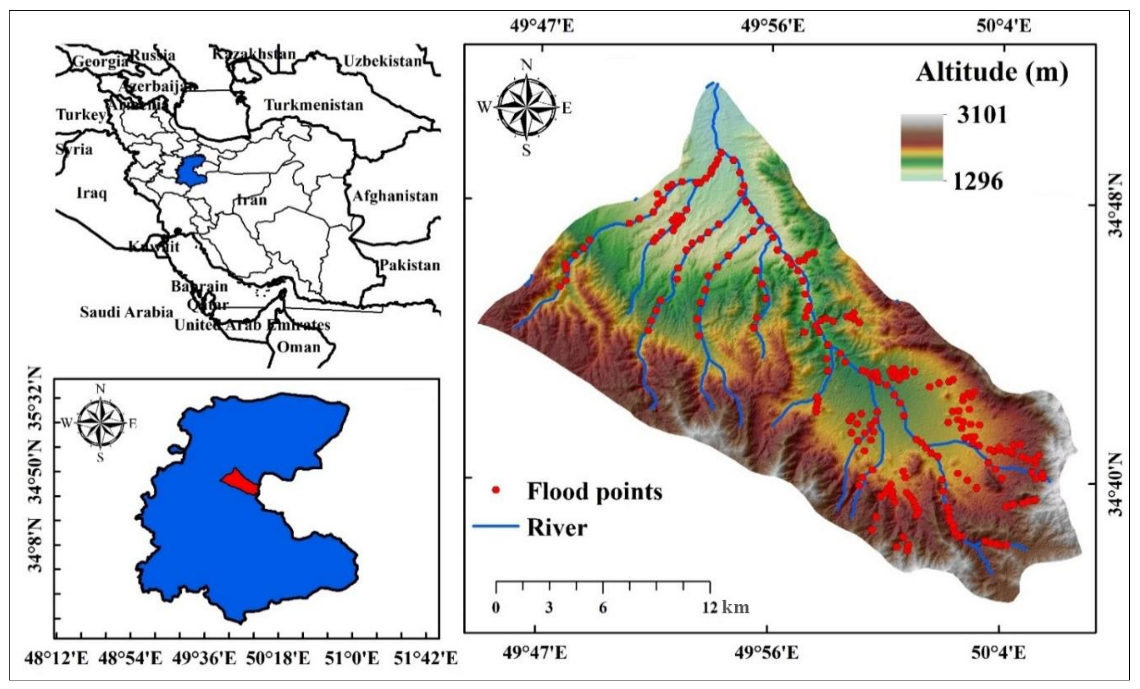
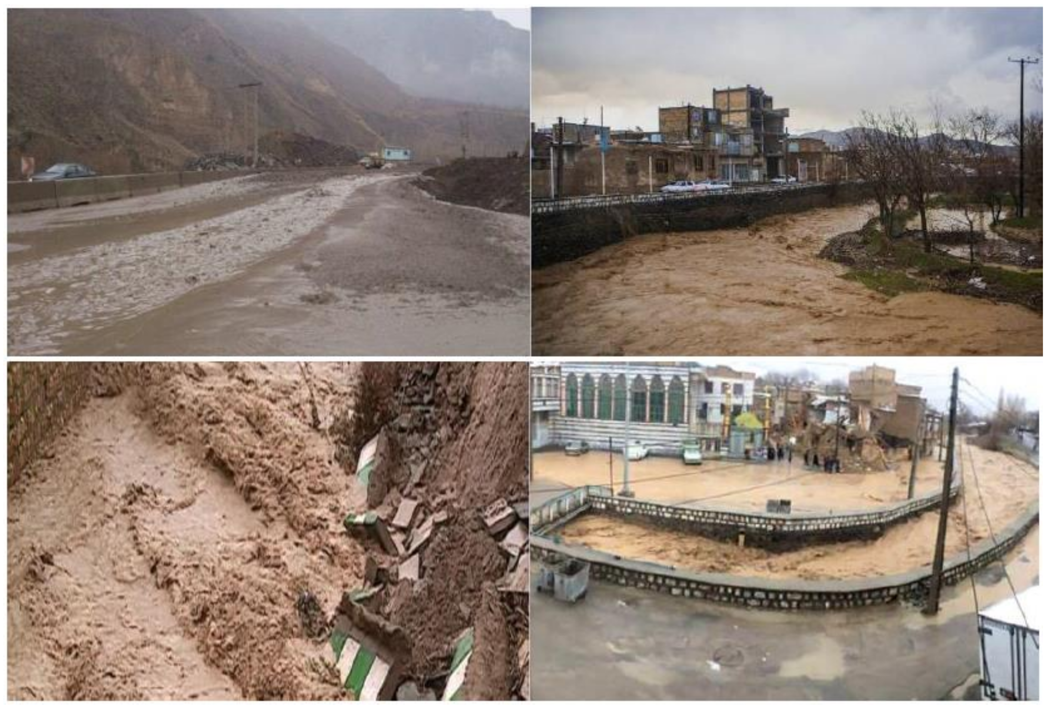
2. Study Area
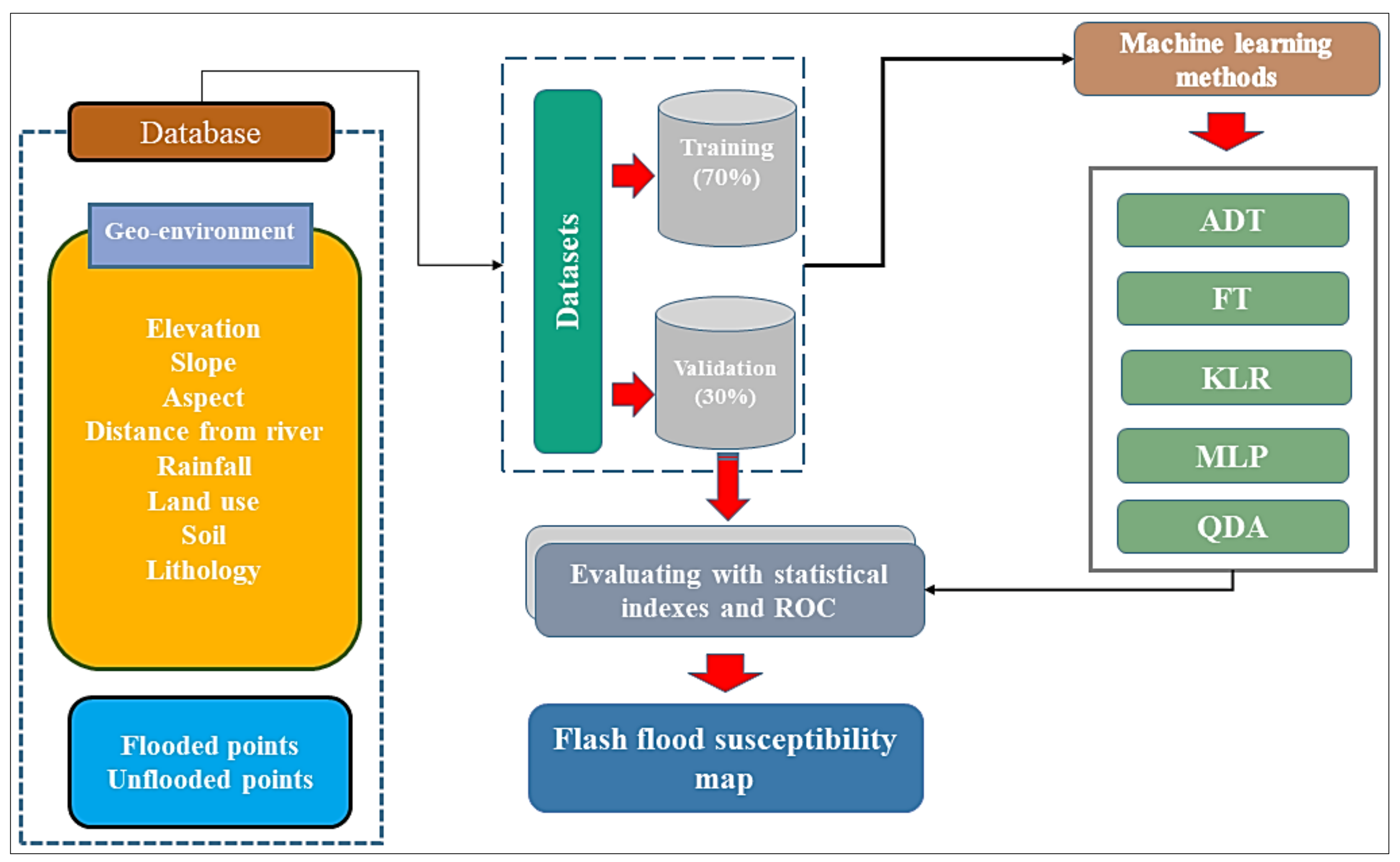
3. Methodology
3.1. Geospatial Database
3.1.1. Inventory Map of Historical Floods
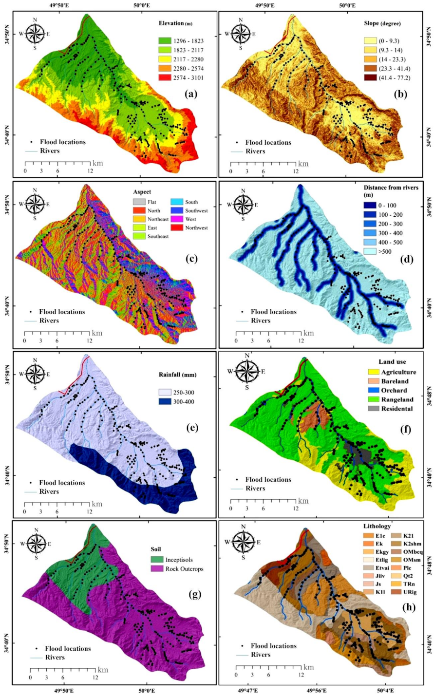
3.1.2. Flood Influencing Factors
3.2. Training and Validation Datasets
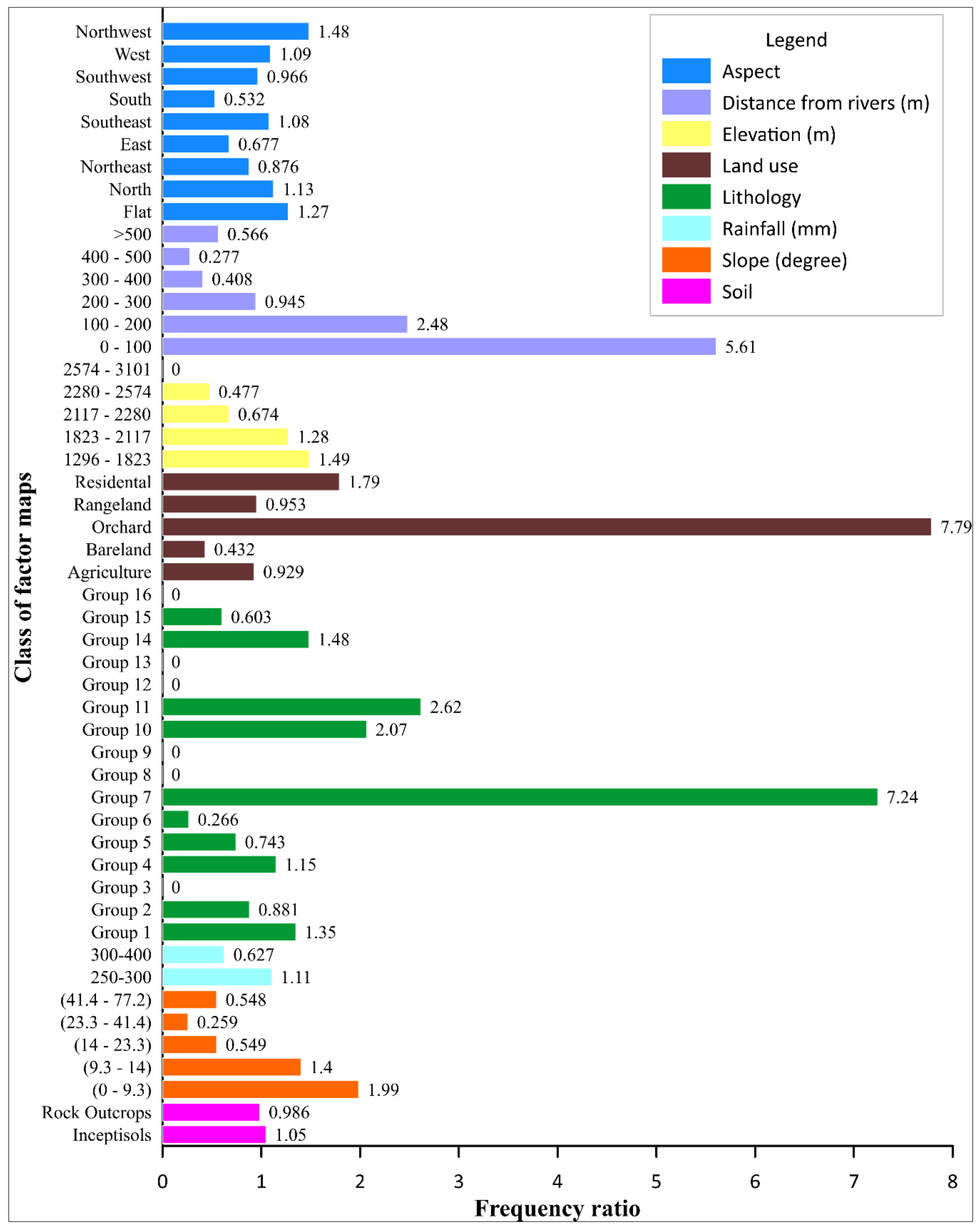
3.3. Spatial Relationship
3.4. Machine Learning Methods
3.4.1. Alternating Decision Tree (ADT)
3.4.2. Functional Tree (FT)
3.4.3. Kernel Logistic Regression (KLR)
3.4.4. Multilayer Perceptron (MLP)
3.4.5. Quadratic Discriminant Analysis (QDA)
3.5. Performance Metrics
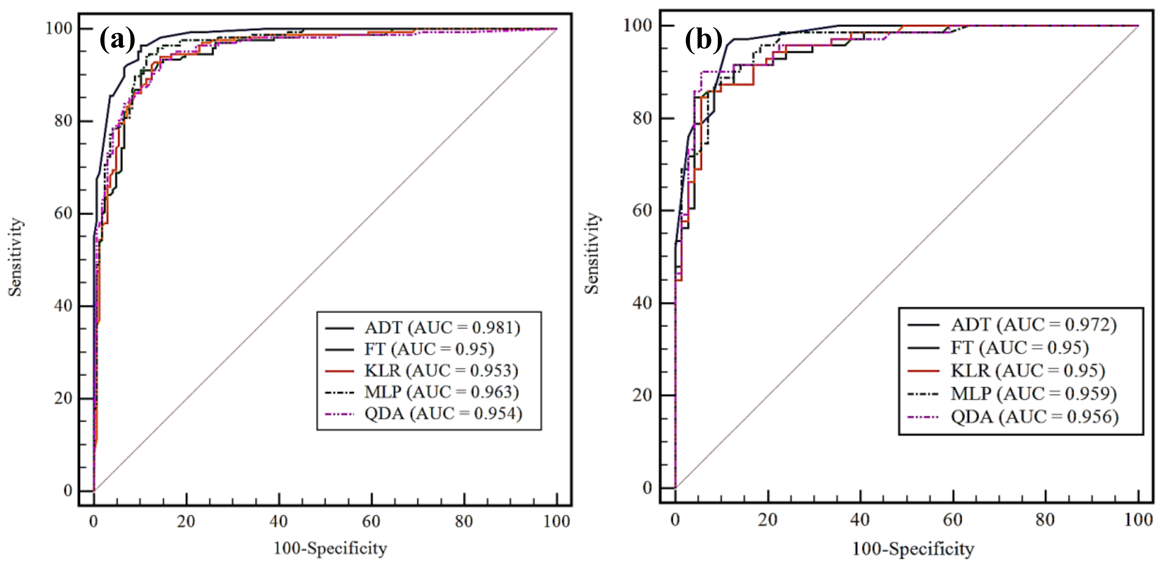
3.5.1. Receiver Operating Characteristic (ROC) Curve
3.5.2. Statistical Indices
4. Results
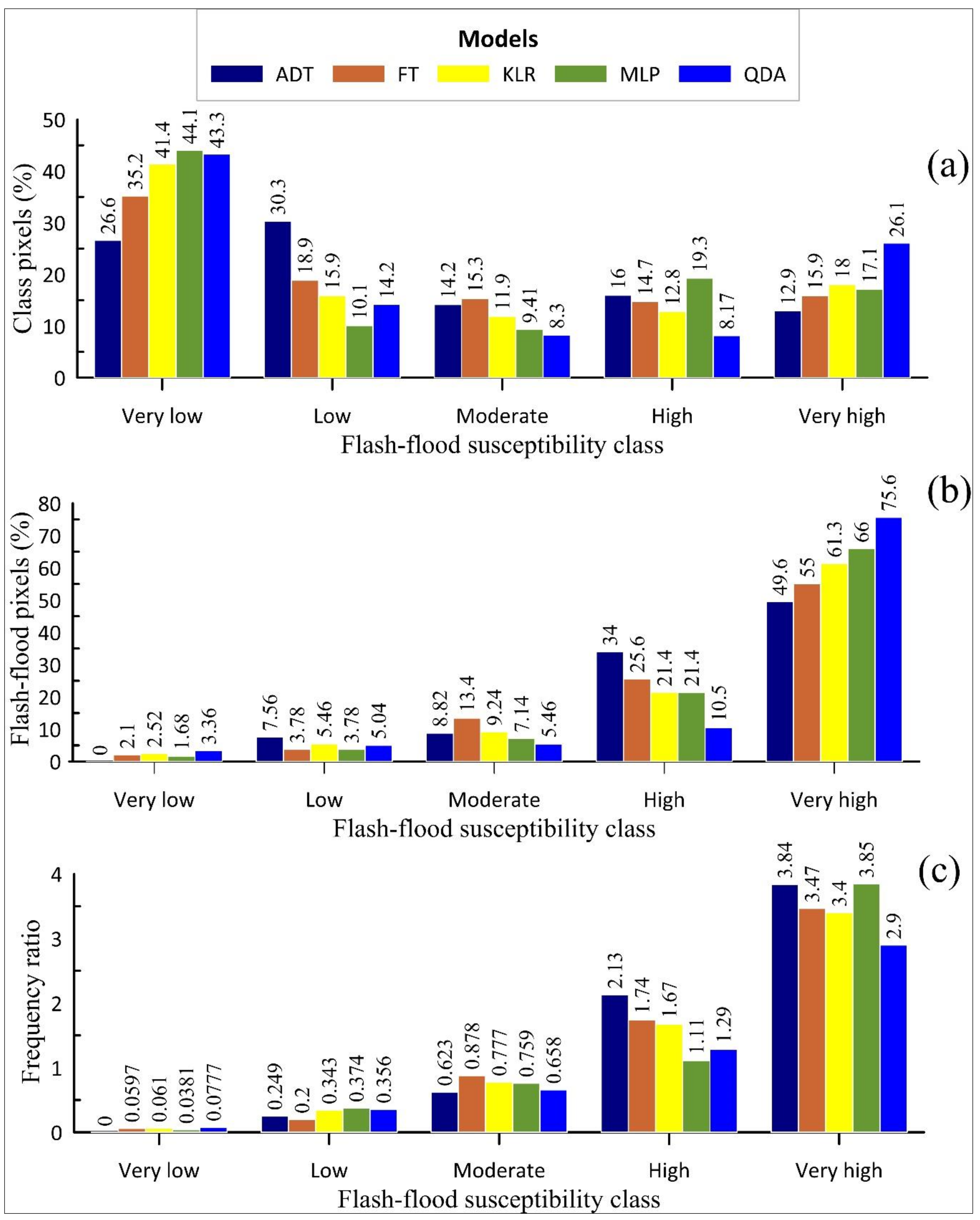
4.1. Spatial Relationship
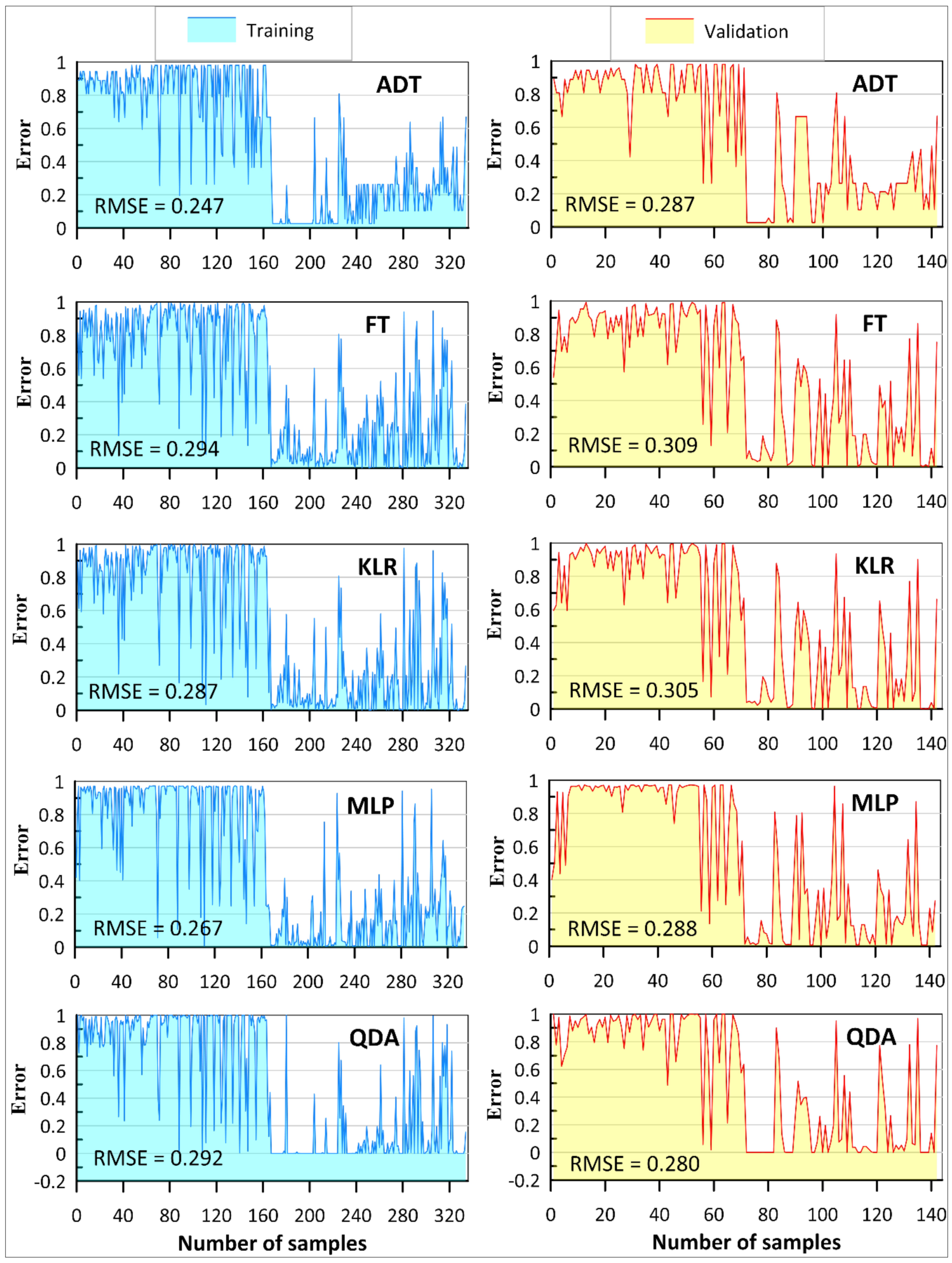
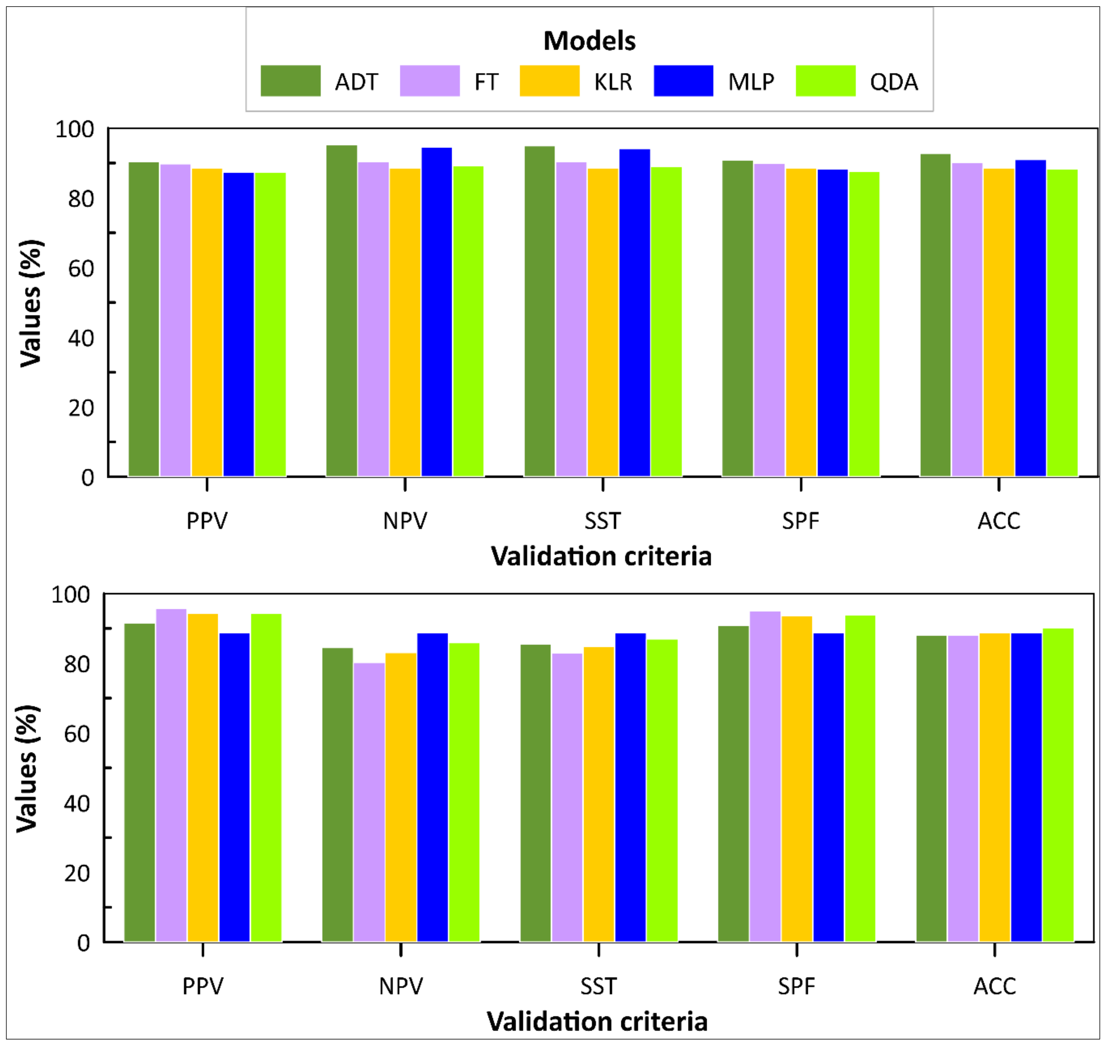
4.2. Model Performance
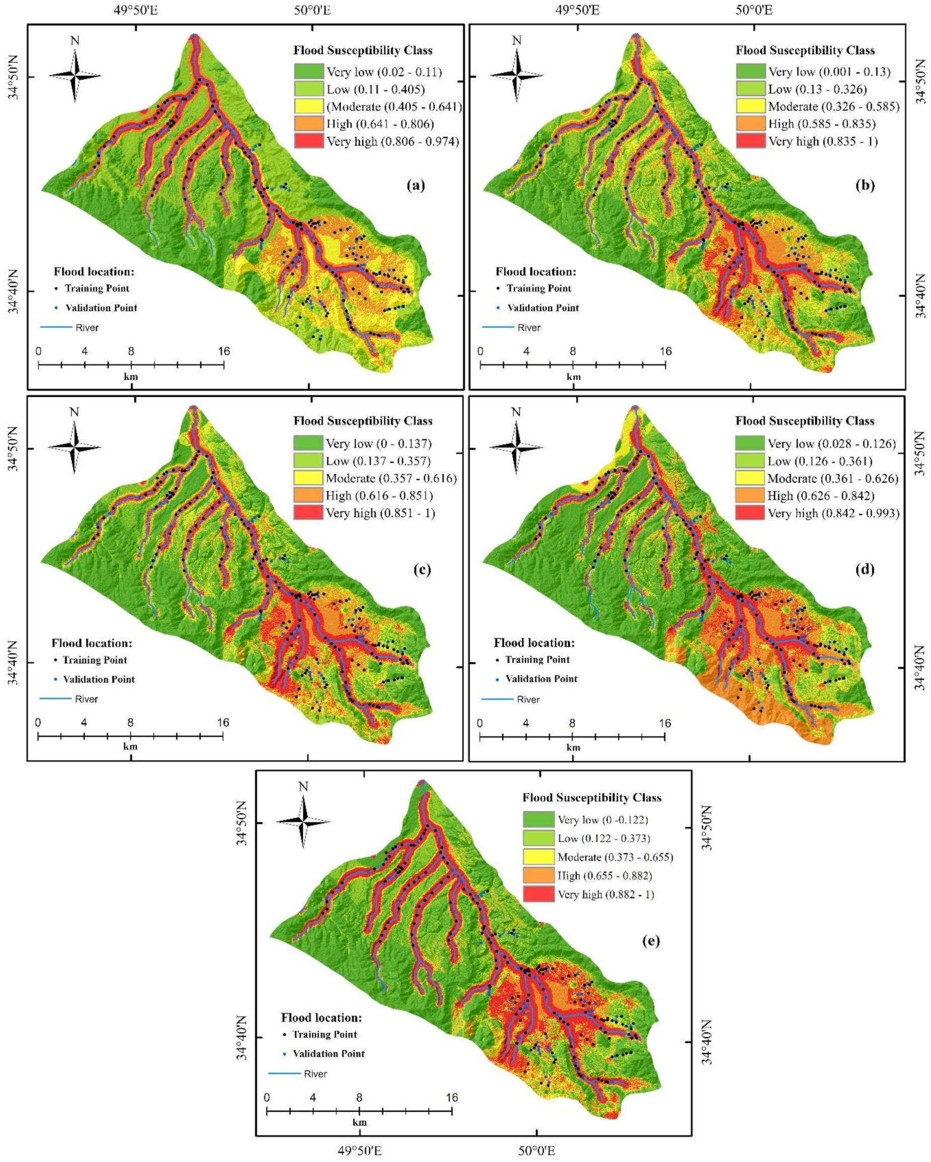
4.3. Flood Susceptibility Maps
5. Discussion and Conclusions
6. Summary
Author Contributions
Funding
Conflicts of Interest
References
- Convertino, M.; Annis, A.; Nardi, F. Information-theoretic portfolio decision model for optimal flood management. Environ. Model. Softw. 2019, 119, 258–274. [Google Scholar] [CrossRef] [Green Version]
- Wright, J.M. Floodplain Management: Principles and Current Practices; The University of Tennessee–Knoxville: Knoxville, TN, USA, 2008. [Google Scholar]
- Wang, X.; Kinsland, G.; Poudel, D.; Fenech, A. Urban flood prediction under heavy precipitation. J. Hydrol. 2019, 577, 123984. [Google Scholar] [CrossRef]
- Dawson, C.W.; Abrahart, R.J.; Shamseldin, A.Y.; Wilby, R.L. Flood estimation at ungauged sites using artificial neural networks. J. Hydrol. 2006, 319, 391–409. [Google Scholar] [CrossRef] [Green Version]
- Tehrany, M.S.; Pradhan, B.; Jebur, M.N. Flood susceptibility mapping using a novel ensemble weights-of-evidence and support vector machine models in GIS. J. Hydrol. 2014, 512, 332–343. [Google Scholar] [CrossRef]
- Bui, D.T.; Ngo, P.T.T.; Pham, T.D.; Jaafari, A.; Minh, N.Q.; Hoa, P.V.; Samui, P. A novel hybrid approach based on a swarm intelligence optimized extreme learning machine for flash flood susceptibility mapping. Catena 2019, 179, 184–196. [Google Scholar] [CrossRef]
- Rahmati, O.; Pourghasemi, H.R.; Zeinivand, H. Flood susceptibility mapping using frequency ratio and weights-of-evidence models in the Golastan Province, Iran. Geocarto Int. 2016, 31, 42–70. [Google Scholar] [CrossRef]
- Chapi, K.; Singh, V.P.; Shirzadi, A.; Shahabi, H.; Bui, D.T.; Pham, B.T.; Khosravi, K. A novel hybrid artificial intelligence approach for flood susceptibility assessment. Environ. Model. Softw. 2017, 95, 229–245. [Google Scholar] [CrossRef]
- Shafizadeh-Moghadam, H.; Valavi, R.; Shahabi, H.; Chapi, K.; Shirzadi, A. Novel forecasting approaches using combination of machine learning and statistical models for flood susceptibility mapping. J. Environ. Manag. 2018, 217, 1–11. [Google Scholar] [CrossRef] [Green Version]
- Amade, N.; Painho, M.; Oliveira, T. Geographic information technology usage in developing countries—A case study in Mozambique. Geo Spat. Inf. Sci. 2018, 21, 331–345. [Google Scholar] [CrossRef]
- Chen, W.; Hong, H.; Li, S.; Shahabi, H.; Wang, Y.; Wang, X.; Ahmad, B.B. Flood susceptibility modelling using novel hybrid approach of reduced-error pruning trees with bagging and random subspace ensembles. J. Hydrol. 2019, 575, 864–873. [Google Scholar] [CrossRef]
- Ahmadisharaf, E.; Kalyanapu, A.J.; Bates, P.D. A probabilistic framework for floodplain mapping using hydrological modeling and unsteady hydraulic modeling. Hydrol. Sci. J. 2018, 63, 1759–1775. [Google Scholar] [CrossRef]
- Aronica, G.; Franza, F.; Bates, P.; Neal, J. Probabilistic evaluation of flood hazard in urban areas using Monte Carlo simulation. Hydrol. Process. 2012, 26, 3962–3972. [Google Scholar] [CrossRef]
- Bates, P.D.; Horritt, M.S.; Aronica, G.; Beven, K. Bayesian updating of flood inundation likelihoods conditioned on flood extent data. Hydrol. Process. 2004, 18, 3347–3370. [Google Scholar] [CrossRef]
- Solomatine, D.P.; Ostfeld, A. Data-driven modelling: Some past experiences and new approaches. J. Hydroinform. 2008, 10, 3–22. [Google Scholar] [CrossRef]
- Moayedi, H.; Tien Bui, D.; Gör, M.; Pradhan, B.; Jaafari, A. The feasibility of three prediction techniques of the artificial neural network, adaptive neuro-fuzzy inference system, and hybrid particle swarm optimization for assessing the safety factor of cohesive slopes. ISPRS Int. J. Geo Inf. 2019, 8, 391. [Google Scholar] [CrossRef]
- Liu, W.K.; Karniakis, G.; Tang, S.; Yvonnet, J. A Computational Mechanics Special Issue on: Data-Driven Modeling and Simulation—Theory, Methods, and Applications; Springer: Berlin, Germany, 2019. [Google Scholar]
- Shafapour Tehrany, M.; Kumar, L.; Neamah Jebur, M.; Shabani, F. Evaluating the application of the statistical index method in flood susceptibility mapping and its comparison with frequency ratio and logistic regression methods. Geomat. Nat. Hazards Risk 2019, 10, 79–101. [Google Scholar] [CrossRef]
- Vojtek, M.; Vojteková, J. Flood Susceptibility Mapping on a National Scale in Slovakia Using the Analytical Hierarchy Process. Water 2019, 11, 364. [Google Scholar] [CrossRef]
- Nandi, A.; Mandal, A.; Wilson, M.; Smith, D. Flood hazard mapping in Jamaica using principal component analysis and logistic regression. Environ. Earth Sci. 2016, 75, 465. [Google Scholar] [CrossRef]
- Khosravi, K.; Shahabi, H.; Pham, B.T.; Adamowski, J.; Shirzadi, A.; Pradhan, B.; Dou, J.; Ly, H.B.; Gróf, G.; Ho, H.L.; et al. A comparative assessment of flood susceptibility modeling using Multi-Criteria Decision-Making Analysis and Machine Learning Methods. J. Hydrol. 2019, 573, 311–323. [Google Scholar] [CrossRef]
- Choubin, B.; Moradi, E.; Golshan, M.; Adamowski, J.; Sajedi-Hosseini, F.; Mosavi, A. An Ensemble prediction of flood susceptibility using multivariate discriminant analysis, classification and regression trees, and support vector machines. Sci. Total Environ. 2019, 651, 2087–2096. [Google Scholar] [CrossRef]
- Kia, M.B.; Pirasteh, S.; Pradhan, B.; Mahmud, A.R.; Sulaiman, W.N.A.; Moradi, A. An artificial neural network model for flood simulation using GIS: Johor River Basin, Malaysia. Environ. Earth Sci. 2012, 67, 251–264. [Google Scholar] [CrossRef]
- Jafarzadegan, K.; Merwade, V. Probabilistic floodplain mapping using HAND-based statistical approach. Geomorphology 2019, 324, 48–61. [Google Scholar] [CrossRef]
- Afshari, S.; Tavakoly, A.A.; Rajib, M.A.; Zheng, X.; Follum, M.L.; Omranian, E.; Fekete, B.M. Comparison of new generation low-complexity flood inundation mapping tools with a hydrodynamic model. J. Hydrol. 2018, 556, 539–556. [Google Scholar] [CrossRef]
- Islamic Republic of Iran Meteorological Organization (IRIMO). 2019. Available online: http://irimo.ir/english/monthly&annual/r25.asp (accessed on 17 February 2019).
- Razi, H.A.; Rad, A.D.; Mardean, M.; Bayat, R. Preparation a corrective-Supplementary Pattern of Watershed Management Programs to Sediment Rate reduce in the Haftan Watershed, Tafresh. Geogr. Environ. Plan. 2016, 61, 1–14. [Google Scholar]
- Darabi, H.; Choubin, B.; Rahmati, O.; Torabi Haghighi, A.; Pradhan, B.; Kløve, B. Urban flood risk mapping using the GARP and QUEST models: A comparative study of machine learning techniques. J. Hydrol. 2019, 569, 142–154. [Google Scholar] [CrossRef]
- Jaafari, A.; Najafi, A.; Rezaeian, J.; Sattarian, A. Modeling erosion and sediment delivery from unpaved roads in the north mountainous forest of Iran. GEM Int. J. Geomath. 2015, 6, 343–356. [Google Scholar] [CrossRef]
- Benito, G.; Rico, M.; Sánchez-Moya, Y.; Sopeña, A.; Thorndycraft, V.; Barriendos, M. The impact of late Holocene climatic variability and land use change on the flood hydrology of the Guadalentín River, southeast Spain. Glob. Planet. Chang. 2010, 70, 53–63. [Google Scholar] [CrossRef]
- Mind′je, R.; Li, L.; Amanambu, A.C.; Nahayo, L.; Nsengiyumva, J.B.; Gasirabo, A.; Mindje, M. Flood susceptibility modeling and hazard perception in Rwanda. Int. J. Disaster Risk Reduct. 2019, 38, 101211. [Google Scholar] [CrossRef]
- Mafi-Gholami, D.; Zenner, E.K.; Jaafari, A.; Ward, R.D. Modeling multi-decadal mangrove leaf area index in response to drought along the semi-arid southern coasts of Iran. Sci. Total Environ. 2019, 656, 1326–1336. [Google Scholar] [CrossRef]
- Bui, D.T.; Tsangaratos, P.; Ngo, P.T.T.; Pham, T.D.; Pham, B.T. Flash flood susceptibility modeling using an optimized fuzzy rule based feature selection technique and tree based ensemble methods. Sci. Total Environ. 2019, 668, 1038–1054. [Google Scholar] [CrossRef]
- Jaafari, A.; Najafi, A.; Pourghasemi, H.R.; Rezaeian, J.; Sattarian, A. GIS-based frequency ratio and index of entropy models for landslide susceptibility assessment in the Caspian forest, northern Iran. Int. J. Environ. Sci. Technol. 2014, 11, 909–926. [Google Scholar] [CrossRef] [Green Version]
- Jaafari, A.; Razavi Termeh, S.V.; Bui, D.T. Genetic and firefly metaheuristic algorithms for an optimized neuro-fuzzy prediction modeling of wildfire probability. J. Environ. Manag. 2019, 243, 358–369. [Google Scholar] [CrossRef] [PubMed]
- Freund, Y.; Mason, L. The alternating decision tree learning algorithm. In Proceedings of the Sixteenth International Conference on Machine Learning (ICML′99), Bled, Slovenia, 27–30 June 1999; Morgan Kaufmann Publishers Inc.: San Francisco, CA, USA, 1999; pp. 124–133. [Google Scholar]
- Gama, J. Functional trees. Mach. Learn. 2004, 55, 219–250. [Google Scholar] [CrossRef]
- Maalouf, M.; Trafalis, T.B.; Adrianto, I. Kernel logistic regression using truncated Newton method. Comput. Manag. Sci. 2011, 8, 415–428. [Google Scholar] [CrossRef]
- Hong, H.; Pradhan, B.; Xu, C.; Tien Bui, D. Spatial prediction of landslide hazard at the Yihuang area (China) using two-class kernel logistic regression, alternating decision tree and support vector machines. Catena 2015, 133, 266–281. [Google Scholar] [CrossRef]
- Chen, W.; Pourghasemi, H.R.; Kornejady, A.; Xie, X. GIS-based landslide susceptibility evaluation using certainty factor and index of entropy ensembled with alternating decision tree models. In Natural Hazards GIS-Based Spatial Modeling Using Data Mining Techniques; Springer: Heidelberg, Germany, 2019; pp. 225–251. [Google Scholar]
- Shawe-Taylor, J.; Cristianini, N. Kernel Methods for Pattern Analysis; Cambridge University Press: Cambridge, UK, 2004. [Google Scholar]
- Bayat, M.; Ghorbanpour, M.; Zare, R.; Jaafari, A.; Thai Pham, B. Application of artificial neural networks for predicting tree survival and mortality in the Hyrcanian forest of Iran. Comput. Electron. Agric. 2019, 164, 104929. [Google Scholar] [CrossRef]
- Tien Bui, D.; Moayedi, H.; Gör, M.; Jaafari, A.; Kok Foong, L. Predicting slope stability failure through machine learning paradigms. ISPRS Int. J. Geo Inf. 2019, 8, 395. [Google Scholar]
- Naghibi, S.A.; Moradi Dashtpagerdi, M. Evaluation of four supervised learning methods for groundwater spring potential mapping in Khalkhal region (Iran) using GIS-based features. Hydrogeol. J. 2017, 25, 169–189. [Google Scholar] [CrossRef]
- Pourghasemi, H.R.; Rahmati, O. Prediction of the landslide susceptibility: Which algorithm, which precision? Catena 2018, 162, 177–192. [Google Scholar] [CrossRef]
- Jaafari, A.; Mafi-Gholami, D.; Pham, B.T.; Tien Bui, D. Wildfire probability mapping: Bivariate vs. multivariate statistics. Remote Sens. 2019, 11, 618. [Google Scholar] [CrossRef]
- Hong, H.; Jaafari, A.; Zenner, E.K. Predicting spatial patterns of wildfire susceptibility in the Huichang County, China: An integrated model to analysis of landscape indicators. Ecol. Indic. 2019, 101, 878–891. [Google Scholar] [CrossRef]
- Jaafari, A.; Panahi, M.; Pham, B.T.; Shahabi, H.; Bui, D.T.; Rezaie, F.; Lee, S. Meta optimization of an adaptive neuro-fuzzy inference system with grey wolf optimizer and biogeography-based optimization algorithms for spatial prediction of landslide susceptibility. Catena 2019, 175, 430–445. [Google Scholar] [CrossRef]
- Jaafari, A. LiDAR-supported prediction of slope failures using an integrated ensemble weights-of-evidence and analytical hierarchy process. Environ. Earth Sci. 2018, 77, 42. [Google Scholar] [CrossRef]
- Jaafari, A.; Zenner, E.K.; Pham, B.T. Wildfire spatial pattern analysis in the Zagros Mountains, Iran: A comparative study of decision tree based classifiers. Ecol. Inf. 2018, 43, 200–211. [Google Scholar] [CrossRef]
- Pham, B.T.; Jaafari, A.; Prakash, I.; Singh, S.K.; Quoc, N.K.; Bui, D.T. Hybrid computational intelligence models for groundwater potential mapping. Catena 2019, 182, 104101. [Google Scholar] [CrossRef]
- Khosravi, K.; Pham, B.T.; Chapi, K.; Shirzadi, A.; Shahabi, H.; Revhaug, I.; Prakash, I.; Tien Bui, D. A comparative assessment of decision trees algorithms for flash flood susceptibility modeling at Haraz watershed, northern Iran. Sci. Total Environ. 2018, 627, 744–755. [Google Scholar] [CrossRef] [PubMed]
- Costache, R. Flash-flood Potential Index mapping using weights of evidence, decision Trees models and their novel hybrid integration. Stoch. Environ. Res. Risk Assess. 2019, 33, 1375–1402. [Google Scholar] [CrossRef]
- Mosavi, A.; Ozturk, P.; Chau, K.-W. Flood prediction using machine learning models: Literature review. Water 2018, 10, 1536. [Google Scholar] [CrossRef]
- Ahmadlou, M.; Karimi, M.; Alizadeh, S.; Shirzadi, A.; Parvinnejhad, D.; Shahabi, H.; Panahi, M. Flood susceptibility assessment using integration of adaptive network-based fuzzy inference system (ANFIS) and biogeography-based optimization (BBO) and BAT algorithms (BA). Geocarto Int. 2019, 34, 1252–1272. [Google Scholar] [CrossRef]
- Tsakiri, K.; Marsellos, A.; Kapetanakis, S. Artificial Neural Network and Multiple Linear Regression for Flood Prediction in Mohawk River, New York. Water 2018, 10, 1158. [Google Scholar] [CrossRef]
- Tehrany, M.S.; Jones, S.; Shabani, F. Identifying the essential flood conditioning factors for flood prone area mapping using machine learning techniques. Catena 2019, 175, 174–192. [Google Scholar] [CrossRef]
- Ma, M.; Liu, C.; Zhao, G.; Xie, H.; Jia, P.; Wang, D.; Wang, H.; Hong, Y. Flash Flood Risk Analysis Based on Machine Learning Techniques in the Yunnan Province, China. Remote Sens. 2019, 11, 170. [Google Scholar] [CrossRef]
- Costache, R.; Bui, D.T. Spatial prediction of flood potential using new ensembles of bivariate statistics and artificial intelligence: A case study at the Putna river catchment of Romania. Sci. Total Environ. 2019, 691, 1098–1118. [Google Scholar] [CrossRef]
- Bui, D.T.; Shirzadi, A.; Shahabi, H.; Chapi, K.; Omidavr, E.; Pham, B.T.; Asl, D.T.; Khaledian, H.; Pradhan, B.; Panahi, M.; et al. A novel ensemble artificial intelligence approach for gully erosion mapping in a semi-arid watershed (Iran). Sensors 2019, 19, 2444. [Google Scholar] [CrossRef]
- Hall, M.; Frank, E.; Holmes, G.; Pfahringer, B.; Reutemann, P.; Witten, I.H. The WEKA data mining software: An update. ACM SIGKDD Explor. Newsl. 2009, 11, 10–18. [Google Scholar] [CrossRef]
- Ahmadisharaf, E.; Kalyanapu, A.; Chung, E.-S. Sustainability-based flood hazard mapping of the Swannanoa River watershed. Sustainability 2017, 9, 1735. [Google Scholar] [CrossRef]
- de Brito, M.M.; Evers, M.; Almoradie, A.D.S. Participatory flood vulnerability assessment: A multi-criteria approach. Hydrol. Earth Syst. Sci. 2018, 22, 373–390. [Google Scholar] [CrossRef]
- Ahmadisharaf, E.; Camacho, R.A.; Zhang, H.X.; Hantush, M.M.; Mohamoud, Y.M. Calibration and validation of watershed models and advances in uncertainty analysis in TMDL studies. J. Hydrol. Eng. 2019, 24, 03119001. [Google Scholar] [CrossRef]


| No. | Geo-unit | Description | Age |
|---|---|---|---|
| 1 | OMsm | Limestone, marl, gypsiferous marl, sandy marl and sandstone (QOM FM) | Oligocene–Miocene |
| 2 | URig | Red marl, gypsiferous marl, sandstone and conglomerate (Upper red Fm) | Miocene |
| 3 | Plc | Polymictic conglomerate and sandstone | Pliocene |
| 4 | Etvai | Dacitic to Andesitic volcano sediment | Eocene |
| 5 | OMbcq | Basal conglomerate and sandstone | Oligocene |
| 6 | Etlig | Andesitic to basaltic volcanic tuff | Eocene |
| 7 | Ek | Well-bedded green tuff and tuffaceous shale (KARAJ FM) | Eocene |
| 8 | EKgy | Gypsum | Late Eocene |
| 9 | Jiiv | Upper Jurassic diorite | Late Jurassic |
| 10 | E1c | Pale-red, polygenic conglomerate and sandstone | Paleocene–Eocene |
| 11 | K1l | Thick-bedded to massive, white to pinkish orbitolina-bearing limestone (TIZKUH FM) | Early Cretaceous |
| 12 | K2l | Hyporite-bearing limestone (Senonian) | Late Cretaceous |
| 13 | K2shm | Shale, calcareous shale and sandstone with intercalations of limestone | Late Cretaceous |
| 14 | Qt2 | Low level piedmont fan and valley terrace deposits | Quaternary |
| 15 | TRn | Sandstone, quartz arenite, shale and fossiliferous limestone (NAIBAND FOR) | Mesozoic |
| 16 | Js | Dark grey shale and sandstone (SHEMSHAK FM) | Triassic–Jurassic |
| Model | Training | Validation |
|---|---|---|
| ADT | 0.856 | 0.761 |
| FT | 0.802 | 0.761 |
| KLR | 0.772 | 0.775 |
| MLP | 0.820 | 0.775 |
| QDA | 0.766 | 0.803 |
© 2019 by the authors. Licensee MDPI, Basel, Switzerland. This article is an open access article distributed under the terms and conditions of the Creative Commons Attribution (CC BY) license (http://creativecommons.org/licenses/by/4.0/).
Share and Cite
Janizadeh, S.; Avand, M.; Jaafari, A.; Phong, T.V.; Bayat, M.; Ahmadisharaf, E.; Prakash, I.; Pham, B.T.; Lee, S. Prediction Success of Machine Learning Methods for Flash Flood Susceptibility Mapping in the Tafresh Watershed, Iran. Sustainability 2019, 11, 5426. https://0-doi-org.brum.beds.ac.uk/10.3390/su11195426
Janizadeh S, Avand M, Jaafari A, Phong TV, Bayat M, Ahmadisharaf E, Prakash I, Pham BT, Lee S. Prediction Success of Machine Learning Methods for Flash Flood Susceptibility Mapping in the Tafresh Watershed, Iran. Sustainability. 2019; 11(19):5426. https://0-doi-org.brum.beds.ac.uk/10.3390/su11195426
Chicago/Turabian StyleJanizadeh, Saeid, Mohammadtaghi Avand, Abolfazl Jaafari, Tran Van Phong, Mahmoud Bayat, Ebrahim Ahmadisharaf, Indra Prakash, Binh Thai Pham, and Saro Lee. 2019. "Prediction Success of Machine Learning Methods for Flash Flood Susceptibility Mapping in the Tafresh Watershed, Iran" Sustainability 11, no. 19: 5426. https://0-doi-org.brum.beds.ac.uk/10.3390/su11195426