Air Quality Trend of PM10. Statistical Models for Assessing the Air Quality Impact of Environmental Policies

Abstract

A statistical modelling of PM10 concentration (2006–2015) is applied to understand the behaviour, to know the influence of the variables to exposure risk, to treat the missing data to evaluate air quality, and to estimate data for those sites where they are not available. The study area, Castellón region (Spain), is a strategic area in the framework of EU pollution control. A decrease of PM10 is observed for industrial and urban stations. In the case of rural stations, the levels remain constant throughout the study period. The contribution of anthropogenic sources has been estimated through the PM10 background of the study area. The behaviour of PM10 annual trend is tri-modal for industrial and urban stations and bi-modal in the case of rural stations. The EU Normative suggests that 90% of the data per year are necessary to control air quality. Thus, interpolation statistical methods are presented to fill missing data: Linear Interpolation, Exponential Interpolation, and Kalman Smoothing. This study also focuses on testing the goodness of these methods in order to find the ones that better approach the gaps. After analyzing graphically and using the RMSE the last method is confirmed to be the best option.

1. Introduction

Due to rapid industrialization, air quality is recognized to be an issue of primary importance for human health. Scientific studies have suggested links between air pollutants and numerous health problems [1,2,3,4]. Thereby, the neediness of improvement air quality in terms of pollutants concentration reduction is essential. In order to deal with this issue, it is necessary to identify and implement long-term air pollution abatement strategies [5]. In this way, the European Union (EU) Framework supplies useful information on air quality assessment techniques, establishes limit values of the pollutants, and urges to develop Air Quality Plans, in particular through Directive 2008/50/EC [6] of the European Parliament and of the Council on ambient air quality and cleaner air for Europe [6] (amended by 2015/1480/EC [7]).

In order to develop Air Quality Plans is essential to know properly the concentrations of the different several pollutants. The EU normative (Directive 2008/50/EC [6], amended by 2015/1480/EC [7]) suggests that 90% of the data per year are necessary, and where possible, modelling techniques should be applied to enable point data to be interpreted in terms of geographical distribution of concentration. This could serve as a basis for calculating the collective exposure of the population living in the area. The results of modelling shall be taken into account for the assessment of air quality with respect to the target values.

In this context, a spatio-temporal modelling of PM10 (particles < 10 $\mathsf{\mu }$m) concentration is applied to understand the trend, to know the influence of the variables to exposure risk, to find the missing data to evaluate air quality, and to estimate data for those sites where they are not available. In addition, it is a useful tool to reduce the number of the sampling points or the days of sampling when there is not enough equipment. This assessment is essential to improve air quality policies and warning alert systems.

The lack of information in time series for each of the monitoring stations makes it difficult to analyse and manage statistics. Previously, statistical methods have been used to predict the concentration of PM10 over time [8,9,10,11]. The aim of this study is to fill missing data by using interpolation statistical methods. The study also focuses on testing the goodness of these methods in order to find the one that better approaches the gaps. After comparing the results of the methods employed through the correlation analysis, the best matching method to restore missing data is chosen.

2. Description of the Study Area

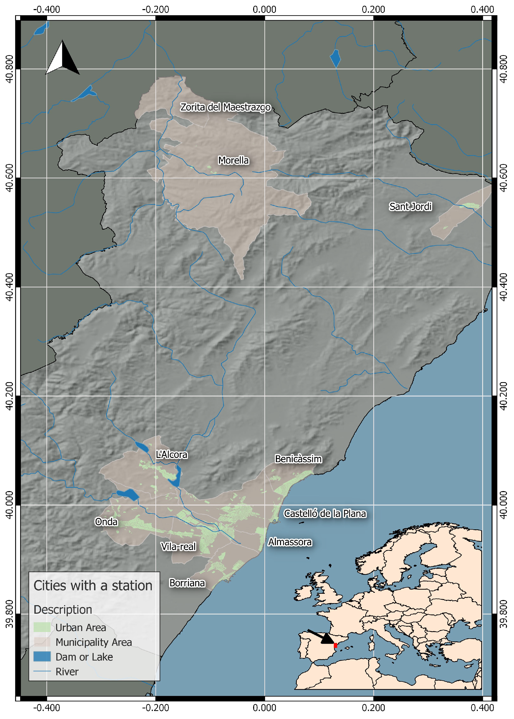
The study area is one of 50 provinces administratively dividing Spain, located in the east of Spain (Figure 1) called Castellón. With 6632 Km${}^2$ and 587,327 inhabitant, this province has a density of 87.81 inhabitants/Km${}^2$ distributed unevenly inside territory, namely, the 85% of the residents live on the coast, 60% in the metropolitan area, and 30% in the capital (INE 2015, Spanish Statistical Office, www.ine.es).

A Mediterranean climate defines this area, a variety of subtropical climate characterized by wet and mild winters, dry and hot summers, and with a mean temperature around 17 ${}^{\circ }$C in coastal areas. Temperatures are colder in the inland, and rainfall in winter is in the form of snow around 600 mm. At the coast, the annual rainfall is around 500 mm, it is abundant in spring and autumn. Summer is prevailed by Azores anticyclone [12].

This area has a complex atmospheric environment with a system of local breezes due to geographical characteristics and the proximity to the sea. These periodic land-sea winds have been extensively studied by several authors [13,14,15,16]. Thus, the concentration of the different pollutants may be affected by the emission of contamination sources located outside of the study area on a daily basis.

The natural source of PM10 in this area is the resuspension of mineral materials from the surrounding mountains with a poor vegetation cover due to the low rainfall. Soil erosion is a concern for air quality. In fact, the study area, in the province of Castellón, is located in the geological context of the Iberian Range (Iberian Plate), in the easternmost part of the Aragonese branch, characterized by preferential NW-SE structural alignments. The geologic materials that predominate are mainly sedimentary materials. Firstly, carbonates (limestones and dolomites), followed by sandstones and lutites and to a lesser extent gypsum. Standing out that towards the coast there is a considerable extension of quaternary deposits of colluvial and alluvial origin that form the great glacis of La Plana (the plain area). On the other hand, in a more local and less widespread way, some ancient outcrops of Paleozoic metamorphic rocks formed by slates, phyllites and schists appear. Therefore, the phenomena of resuspension of mineral particulate matter in the atmosphere would be mainly associated to: clay, quartz, calcite, dolomite, hematite and gypsum minerals. Low rainfall favours the long residence time of particles from these geological materials. Moreover, considering the presence of a nearby coast, the PM10 concentrations are also affected by sea spray. It is produced by bubble-bursting processes when wind hits the surface of the ocean and waves occur. Small bubbles are formed, which discharge liquid particles in the range of submicrometre size up a few micrometres. These particles projected at very high speeds are incorporated into the masses of moving air [17]. In addition, it is important to consider the long-range transport of materials from North Africa [18,19]. These dust intrusions from North Africa influence ambient PM10 levels in the study area at around 2 $\mathsf{\mu }$g/m${}^3$ on an annual basis [20].

Anthropogenic pollution sources originate from automobile traffic (mobile sources) and industrial activity (fixed sources). The urban and industrial development of Castellón region is especially prominent, causing heavy and complex air pollution problems as many research articles have reported [21,22]. This region is a strategic area in the framework of European Union (EU) pollution control. It is the first manufacturer and exporter of ceramics tiles in the EU. This industrial sector has an important feature, which is a large concentration of manufacturers in a tiny space. In addition, at the East of the study area, there is a thermal power plant (coal gasification integrated in a combined cycle), a refinery and several chemical industries. These industries together contribute to environmental pollution in the small area.

3. Methodology

3.1. Data Collection

The measurements conducted by “Red Valenciana de Vigilancia y Control de la Contaminación Atmosféric” of “Conselleria de Agricultura, Medio Ambiente, Cambio Climático y Desarrollo Rural, Generalitat Valencian” are used in this analysis to assess air quality status in the Castellón region. The management of the sampling fulfils European Directive 2008/50/EC [6] (amended by 2015/1480/EC [7]) on ambient air quality and cleaner air for Europe. Firstly, Figure 1 shows the network location of stations which monitors air quality levels for PM10 in the period 2006–2015, and secondly,

Table 1. Characteristics of the monitoring stations

Station	Character	Longitude	Latitude	Altitude (m)
Almassora	Industrial	751,611	4,424,616	27
L’Alcora	Industrial	738,204	4,439,125	160
Onda	Industrial	734,893	4,427,323	163
Vila-real	Industrial	747,285	4,425,370	60
Benicàssim	Urban	250,329	4,438,460	50
Borriana	Urban	750,955	4,419,994	37
Castellón de la Plana	Urban	753,900	4,430,805	18
Morella	Rural	758,888	4,502,629	1153
Sant Jordi	Rural	277,544	4,492,723	181
Zorita	Rural	739,030	4,513,273	619

shows the characteristics of the monitoring stations.

3.2. Modelling Tool

A common problem encountered in time series analysis evaluating air quality is the scarcity or nonexistence of current daily or historical measurements. Missing data in time series analysis may lead to a biased estimation of the pollutants and perform erroneous air quality assessment, which means that a more suitable solution is needed in order to create results that are more realistic.

The mentioned restriction urges to fill the data gaps by using statistical methods, and after testing different alternatives and reviewing interpolation methods used to fill gaps in time-series in the literature [23,24,25], we focused on three interpolation methods (a) Linear Interpolation (LI) [26,27], (b) Exponential Weighted Moving Average (EWMA) model [28] and (c) Kalman Smoothing on structural time series model (KS-StructTS), as these were the ones that better commit with our data. The first one is characterized for returning a list of points (x,y) which linearly interpolate given data points. The next one reduces influences by ranking first recent data points and addresses both of the problems associated with the simple moving average as prioritises recent data. The Kalman Smoothing applies to a structural model for a time series by maximum likelihood [29,30,31].

In order to better understand differences between these three methods a correlation analysis was carried out by performing three plots considering the correlation between two methods each time. All the interpolation methods have been managed by the free R software [32].

4. Results and Discussion

4.1. PM10 Trends

A comparison of PM10 levels was carried out at different points in the Castellón region, and Figure 2 shows the blox-pot of the data of all stations in the study period (2006–2015). The three typologies of stations are significantly different confirmed with an anova test. Industrial stations present higher levels than the others and rural stations have the least PM10 concentrations although Zorita presents a higher value than all distributions which justifies studying the trend in order to assess the variables that influence it.

4.1.1. PM10 Background

It is very important to know the regional background in order to estimate the contribution of anthropogenic sources. The data used for estimating the regional background are from monitoring stations located in the countryside at some distance from anthropogenic PM emission sources and urban nuclei. European Community has stabled some stations of this type throughout its territory through the EMEP, Cooperative Programme for the Monitoring and Evaluation of Long Range Transmission of Air Pollutants in Europe. The EMEP is a scientifically based and policy-driven program under the Convention on Long-range Transboundary Air Pollution (CLRTAP) for international co-operation to tackle transboundary air pollution problems. Ten EMEP stations are currently operative in Spain, distributed all over the country [33].

In the study area, the Morella station could be considered a background EMEP program station as it adjusts to its parameters (see criterion in Van Dingenen et al. [34]), and in the study period (2006–2015) the annual mean of PM10 ranges 8–14 $\mathsf{\mu }$g/m${}^3$. Van Dingenen et al. [34] in 2004 determined the European continental background concentration about 7.0 $\mathsf{\mu }$g/m${}^3$ and in the same year Querol et al. [33] studied PM10 concentrations at regional background in different EMEP station around Spain. They determined regional background around 15 $\mathsf{\mu }$g/m${}^3$ in Galicia, Euskadi and central Spain, 17 $\mathsf{\mu }$g/m${}^3$ in Andalucia and 19 $\mathsf{\mu }$g/m${}^3$ in Canary Island. The regional background in the study area is over European continental background concentration and in the same range of the other region of Spain. Being in mind the annual average data of Castellón region, there is a difference between Morella station and industrial and urban stations about 15 $\mathsf{\mu }$g/m${}^3$, and 5 $\mathsf{\mu }$g/m${}^3$ from the other rural stations. These differences are attributable to anthropogenic sources.

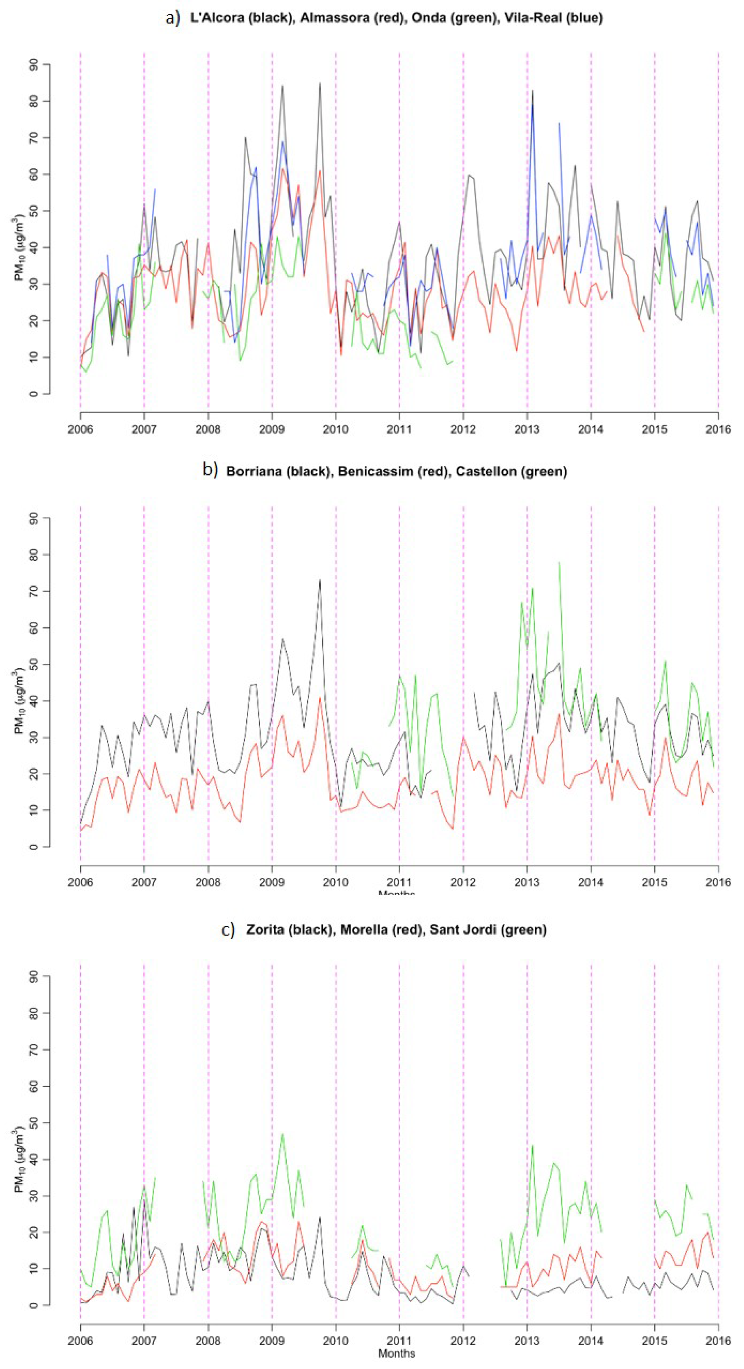
4.1.2. PM10 Spatio-Temporal Trend

Figure 3 presents the PM10 concentration of all stations in the study period (2006–2015) for available measurements. A general decrease of PM10 concentration levels over the study period is observed in the case of industrial and urban stations due to economic crisis. A consequence of the economic recession is a reduction of industrial production in this area and therefore, a decrease in traffic is observed (

Table 2. Production of ceramic industries processes and traffic data in Castellón Region. Tile production, gas and electric consumption are extracted from the ASCER (Spanish Ceramic Tile Manufacturers’ Association) website (www.ascer.es). Comulative traffic is extracted from Generalitat Valenciana-Conselleria d’Infreaestructures i transport website (www.gva.es).

Year	Tile Production Millions of m${}^2$	Gas Consumption (PCS) GWh	Electric Consumption GWh	Cumulative Traffic Vehicles km
2006	565.8	17,947	1358	1,103,316,501
2007	543.8	17,294	1305	1,307,931,891
2008	460.5	15,438	1104	1,264,157,009
2009	301.7	9616	724	1,085,616,106
2010	340.4	9774	817	1,036,140,610
2011	364.6	10,385	1135	1,111,049,389
2012	375.7	10,928	1170	1,078,875,454
2013	390.6	11,094	1216	1,058,187,852
2014	395.2	11,548	1229	1,116,037,075
2015	409.2	11,897	1274	1,187,119,651

). Along with this line, the main sources of emission have been reduced, not linearly, but with oscillations when activation or deactivation of the local economy takes place. Thereby, it is expected that when the productive processes increase, more pollutants could be emitted and consequently the levels of PM10 could increase. In the case of rural stations, the levels remain constant throughout the study period.

In addition, in Figure 3 it is observed that the behaviour is tri-modal for the case of industrial and urban stations, and bi-modal in the case of rural stations. The two peaks that are coincident in the three types of stations were observed in spring and summer. In these months, rainfall is lower and temperatures are higher which leads to dryness of the terrain, and consequently, there is an increase in the resuspension of the substrate in this area and there are more particles in the air. This fact was also observed by Cesari et al, 2018 [35] in the southern of Italy. In addition, the mixed layer, caused by the vertical heat convection, is increasing that favours the intrusion of particulate matter from long-range transport. 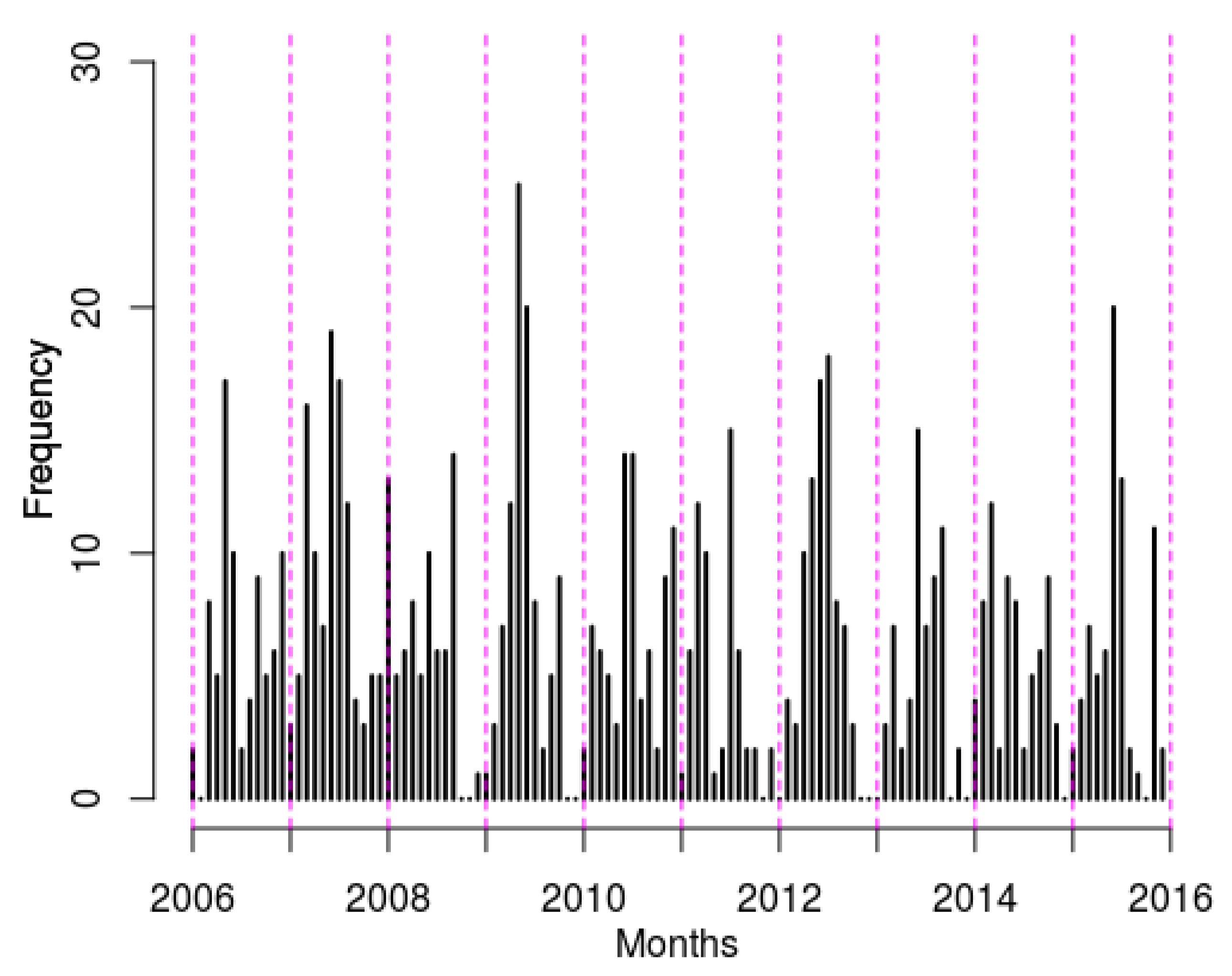The atmospheric dust in the upper layer has the possibility of downward mixing [36,37]. The assessment of PM10 cannot be done with one criterion due to long-range transport of particles from North Africa. Figure 4 shows the frequency per month of this phenomenon over the study area. Mainly, it occurs in spring and summer.

This seasonal pattern is frequently observed from April to August and at the end of the autumn, which coincides with what was observed by Escudero et al. [38]. During these periods, surface winds introduce mineral particles into the atmosphere from African dry soils. Sahara and Sahel areas together entail 99% of North African dust emissions. Sahara emits between 13.4 × 10${}^8$ to 15.7 × 10${}^8$ Tn·year${}^{-1}$ while Sahel 2.3 × 10${}^8$ to 3.8 × 10${}^8$ Tn·year${}^{-1}$[39]. It is calculated that a 12% of this dust is transported northward to Europe [40], therefore about 2 × 10${}^8$ Tn·year${}^{-1}$ arrive at Mediterranean Basin. Initially, this phenomenon induces that the regional background of particles are increased [41], and Querol et al. [42], in 2009 reported that the annual mean levels of PM10 was heightened around 10 $\mathsf{\mu }$g/m${}^3$ in air quality networks from the Eastern Mediterranean, and 2 to 4 $\mathsf{\mu }$g/m${}^3$ in the Western Mediterranean.

The third peak, which is observed in industrial and urban stations, is monitored in winter. During this season, a thermal inversion phenomenon occurs that stabilises the air mass, which reduces turbulence and mixing [43]. Under these conditions, emitted pollutants are accumulated and its concentration increases. The last peak also points out the use of domestic heating (mainly biomass and fuel) that depends on the number of inhabitants of each zone, which fades in rural areas where the density of the population is lower.

4.2. Modelling Results

As previously mentioned, the EU normative (Directive 2008/50/EC [6], amended by 2015/1480/EC [7]) suggests that the 90% of the data per year is necessary to do this assessment. For this reason, it is necessary to formulate a statistical model for estimating the missing data.

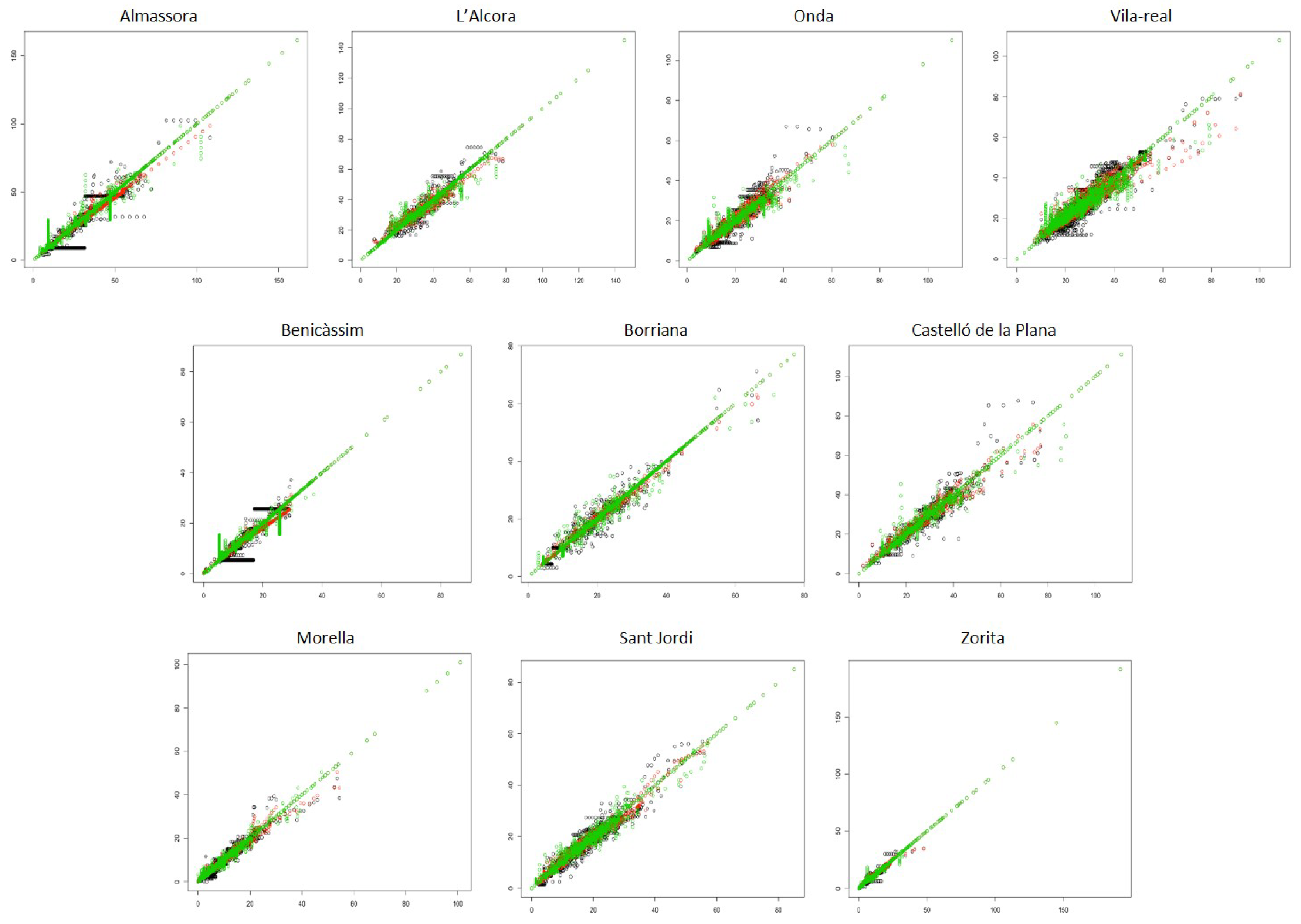
In order to compare interpolation methods with each other, two-to-two correlations have been calculated to analyze their similarity. Thus, in Figure 5 it is shown the correlation graph between two interpolation methods. Black points show the performance between linear interpolation and EWMA; red points between linear interpolation and Kalman Smoothing and green points between EWMA and Kalman Smoothing. Even if we do not observe great differences between them, the EWMA method is the one that differs most from the other two. In particular, analysing the correlation coefficient, even if all of them are statistical significant the highest value correspond to the pair between linear interpolation and Kalman Smoothing. The visual analysis derived from Figure 5 is supported by the values shown in

Table A1. Correlation and RMSE values between two pairs of the three interpolation methods used according to all stations.

Methods	Almazora	Benicassim	Burriana	Castellón	Alcora	Morella	Onda	Sant Jordi	Vila-real	Zorita
LIEWMA
Cor	0.9777595	0.9746722	0.9949086	0.9899099	0.9922703	0.9922337	0.9848897	0.9908656	0.9790503	0.997541
RMSE	3.920448	1.863123	1.863123	1.900147	1.768246	1.029518	1.752061	1.322349	2.72974	0.7283757
LIKS-StructTS
Cor	0.9981235	0.9969114	0.9992442	0.9964016	0.9967184	0.9972584	0.9937334	0.9971758	0.9882882	0.9989981
RMSE	1.158026	0.6561339	0.6561339	1.134342	1.153137	0.6135989	1.101351	0.7378185	2.154658	0.4660446
KS-StructTSEWMA
Cor	0.9793446	0.9731997	0.996001	0.9928308	0.992935	0.9963404	0.9861183	0.994214	0.9825219	0.9978561
RMSE	3.775596	1.9221	1.9221	1.605933	1.696092	0.7046247	1.686347	1.052964	2.546553	0.6806163

(Appendix A). Moreover, this table also includes the RMSE values which show that the lowest values also occur between linear interpolation and Kalman Smoothing methods. Thus, these two methods are those more similar.

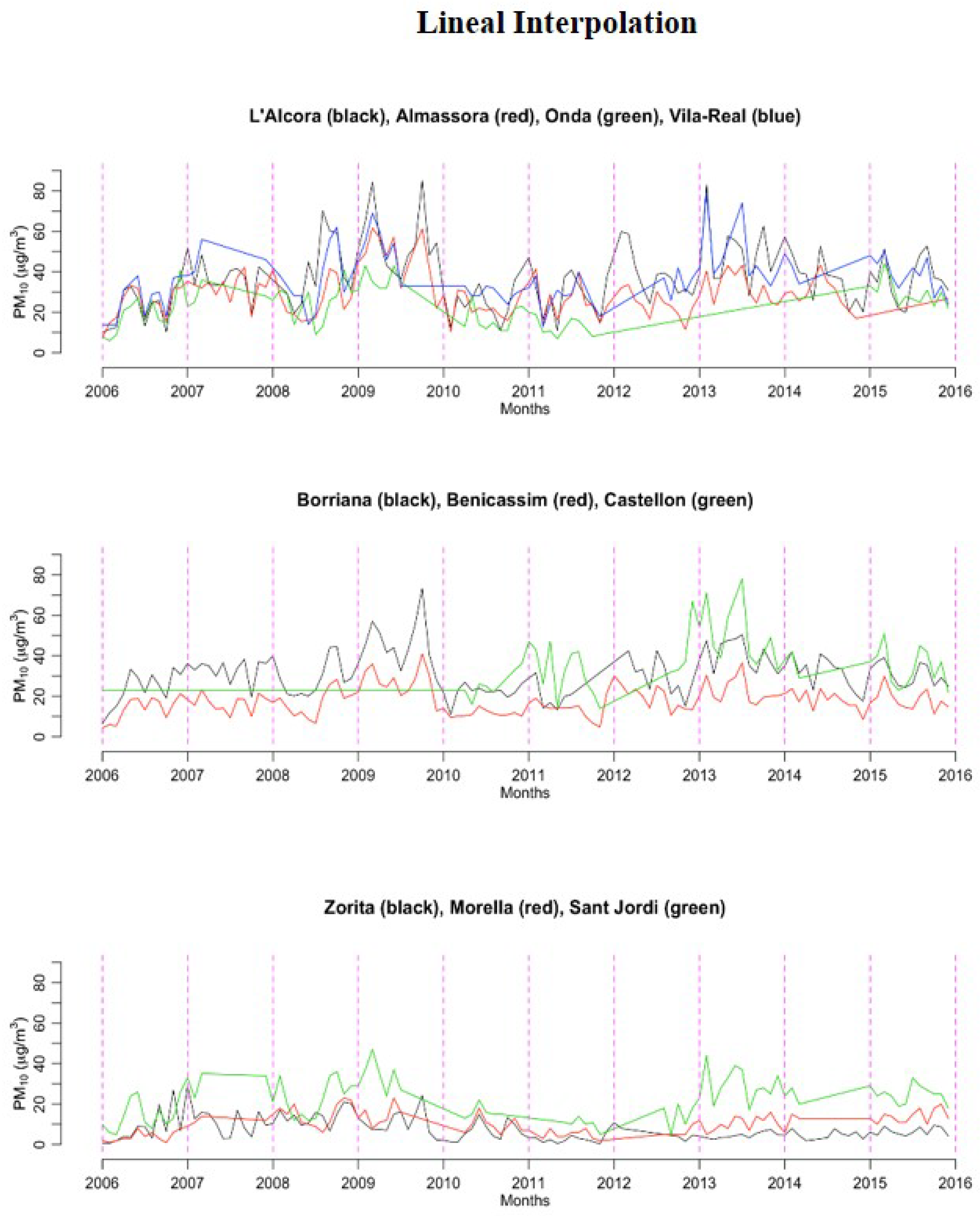
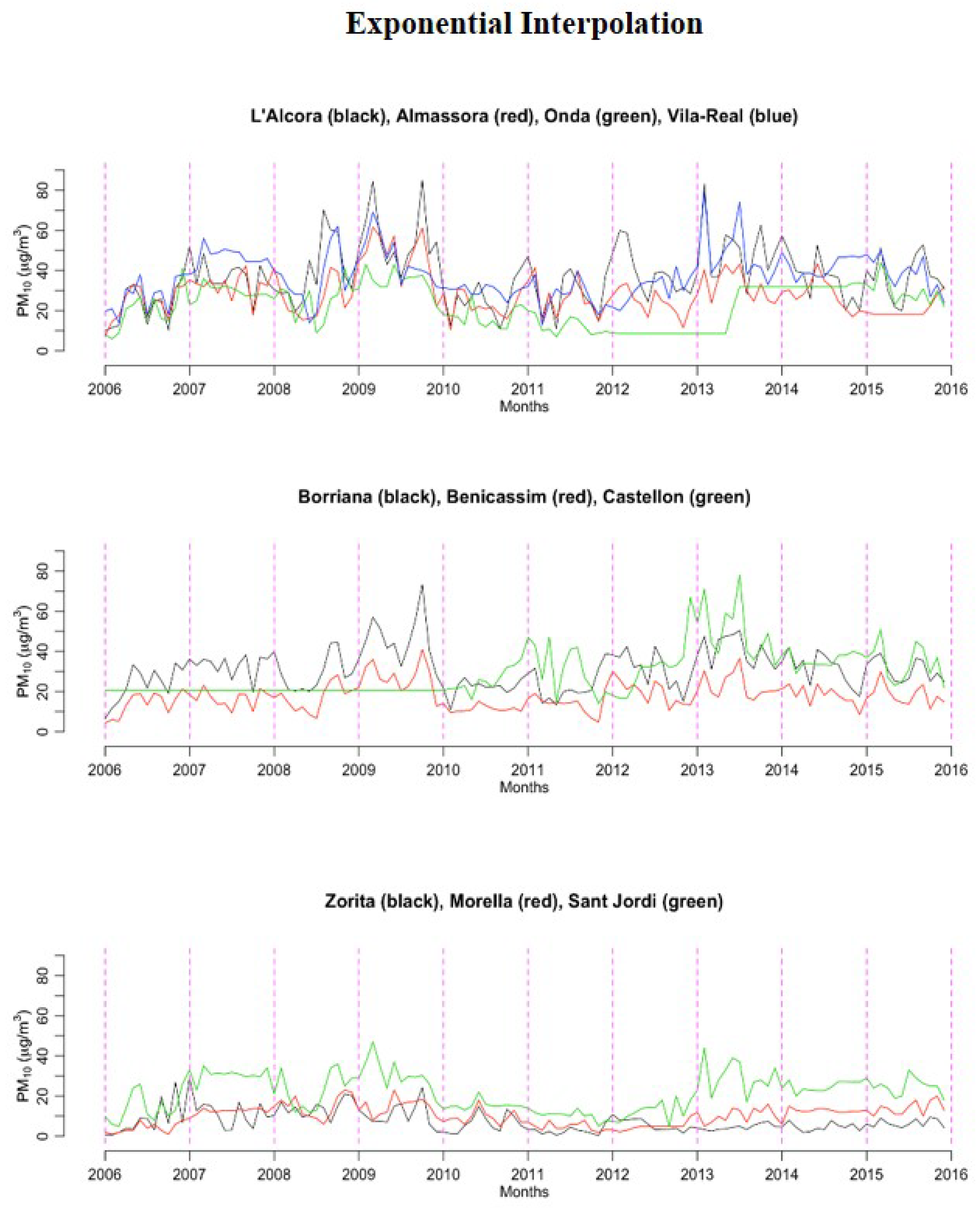
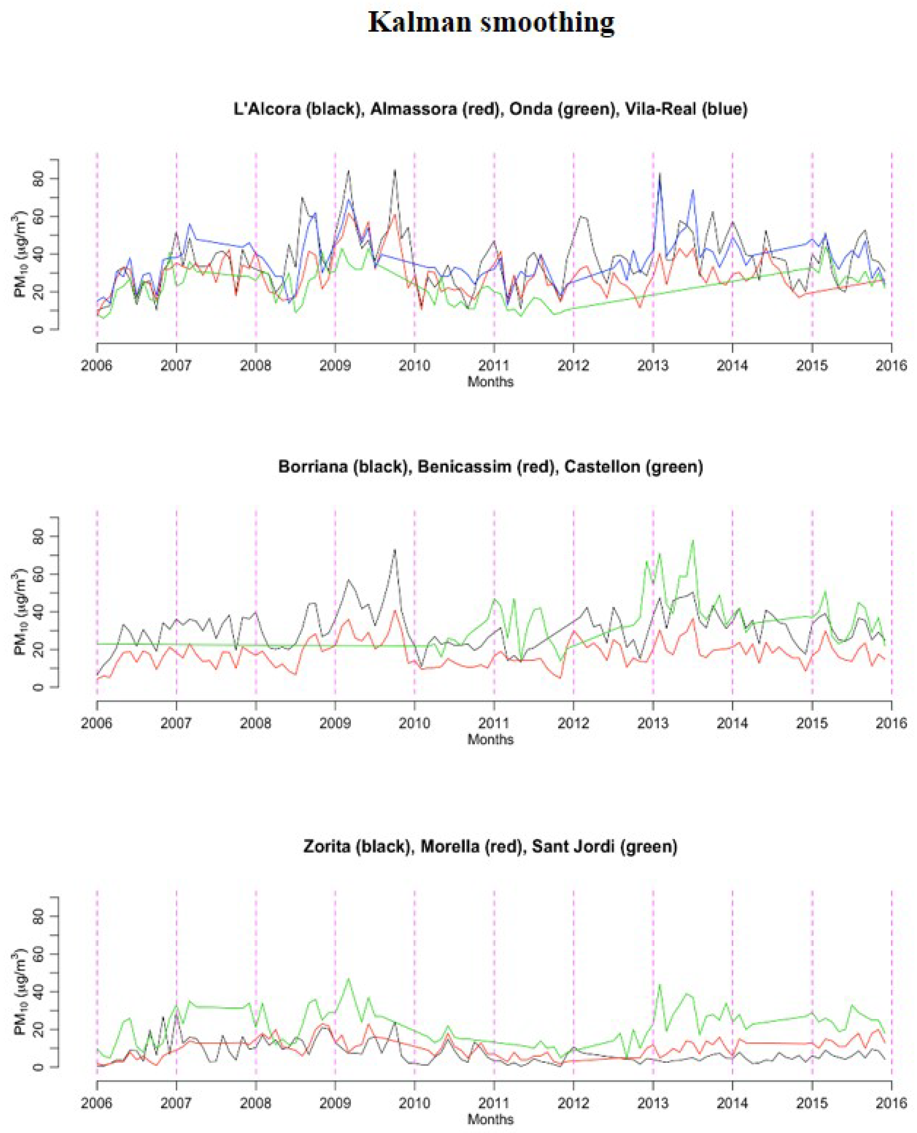
In addition, Figure 6, Figure 7 and Figure 8, which represents both, the initial graph with missing data and the one filling the gaps using an interpolation method, suggests that Kalman Smoothing is usually the best choice for imputation as it is the one which better collects the variations between one gap and another. Linear method is only based on imputing the data following a straight line. When the number of missing is high this methods is not very accurate. The other two methods employed in this research try to impute the missing data considering the entire series and this lead to a better approximation and to a better adjustment. This result is also confirmed with the values shown in

Table A2. RMSE values comparing real data and imputed data for each of the three interpolation methods used and for five of the study stations.

	Almazora	Benicassim	Burriana	Castellón	Zorita
LI	2.725728	2.706501	3.604199	12.295602	2.746331
KS-StructTS	2.709551	2.673490	3.414772	6.547038	2.094441
EWMA	44.081294	2.936913	4.420645	8.967623	1.87483

(Appendix A). It shows how the RMSE, calculated between real data and imputed values, for each of the interpolation methods used, indicate the lowest values for the KAL for five of the study stations.

Nevertheless, the goodness of the interpolation methods depends on the number of missing values of the series. Therefore,

Table 3. Number of missing values for each station.

Station	N(%)
Almassora	784 (21.5)
L’Alcora	477 (13.1)
Onda	813 (22.3)
Vila-real	1912 (52.4)
Benicàssim	710 (19,4)
Borriana	498 (13.6)
Castellón de la Plana	686 (18.8)
Morella	651 (17.8)
Sant Jordi	920 (25.2)
Zorita	476 (13)

, which shows the number of missing values for each station, gives an idea about which stations will be better refilled. It is obvious, than when there are less missing values the fit is better. This is the case of Vila-real. In addition, if the missing values are distributed over the entire study period, the goodness is better. Against, if they are consecutive, the interpolation method does not present a good fit. This is the case of Castellón de la Plana, in the first year the fit is worse than the last.

5. Conclusions

PM10 trend is assessed by 10 monitoring stations with different character through time series of daily data (2006–2015) in Castellón region, Spain. These stations have industrial character, urban and rural; 4, 3 and 3 respectively. To evaluate the air quality in this region, a combination of statistical methods is used in this research to withdraw the missing data.

As a first conclusion, the industrial stations present higher levels of PM10 than the rural stations, which show the lowest levels. An exception of it is Zorita station which presents a higher value than the rest of the distributions. This phenomenon occurs due to natural and anthropogenic sources that influence in each station. Natural sources are the resuspension of mineral material from surrounding mountains and the long-transport of material from North Africa, and anthropogenic sources are traffic and industrial activity since it is the first manufacturer and exporter of ceramic tiles in the EU. In reference to the PM10 regional background, a difference of 15 $\mathsf{\mu }$g/m${}^3$ has been found in the case of industrial and urban stations and 5 $\mathsf{\mu }$g/m${}^3$ in the case of rural stations due to anthropogenic sources in this area. During the study period (2006–2015) a decrease of PM10 levels is observed for industrial and urban monitoring stations due to anthropogenic reduction consequence to economic crisis. In the case of rural stations, the levels remain constant throughout the study period.

A second conclusion is the behaviour of PM10 annual trend is tri-modal for the case of industrial and urban stations, and bi-modal in the case of rural stations. The peaks depend of the general weather conditions, that influence over the resuspension of the mineral material, the long-transport particles from North Africa and the increase of anthropogenic sources when a thermic inversion phenomenon occurs.

The third conclusion of the research is that the spatio-temporal modelling of PM10 concentrations is presented to properly assess the air quality in the study area. Since we do not have the complete data series and to be able to make proper estimations, three interpolation methods have been employed. As the analysis is sensitive to missing values, many efforts have been devoted to the validation of interpolation methods with the intention of minimizing the possible errors that could be created by the imputed values in the trend of the actual values of the PM10 that we are analyzing. For this reason the graphic analysis has been combined with numerical values that confirm the conclusions drawn visually. Thus, after making comparative analyzes between the interpolation methods and studying which one best approximates the data, we have concluded that Kalman Smoothing is, in general, the best option. In addition, it has also been shown that the number of missing values and their distribution in the study period are important factors in order to apply the interpolations methods properly.

References

- Pope, C.A.; Dockery, D.W.; Schwartz, J. Review of epidemiological evidence of health effects of particulate air pollution. Inhal. Toxicol. 1995, 7, 1–18. [Google Scholar] [CrossRef]
- Brunekreef, B.; Holgate, S.T. Air pollution and health. Lancet 2002, 360, 1233–1242. [Google Scholar] [CrossRef]
- Dockery, D.W. Health effects of particulate air pollution. Ann. Epidemiol. 2009, 19, 257–263. [Google Scholar] [CrossRef] [PubMed]
- Lee, J.Y.; Lee, S.B.; Bae, G.N. A review of the association between air pollutant exposure and allergic diseases in children. Atmos. Pollut. Res. 2014, 5, 616–629. [Google Scholar] [CrossRef] [Green Version]
- Moussiopoulos, N. The multi-pollutant cost-effectiveness emission reduction problem. In Proceedings of the 7th International Conference on Protection and Restoration of the Environment, Myconos, Greece, 28 June–1 July 2004. [Google Scholar]
- Official Journal of the European Union; European Commission. Directive 2008/50/EC of the European Parliament and of the Council of 21 May 2008 on Ambient Air Quality and Cleaner Air for Europe; Official Journal of the European Union: Luxembourg, 2008. [Google Scholar]
- Official Journal of the European Union. Directive 2015/1480 of 28 August 2015 Amending Several Annexes to Directives 2004/107/EC and 2008/50/EC of the European Parliament and of the Council Laying Down the Rules Concerning Reference Methods, Data Validation and Location of Sampling Points for the Assessment of Ambient Air Quality; Official Journal of the European Union: Luxembourg, 2008. [Google Scholar]
- Perez, P. Combined model for PM10 forecasting in a large city. Atmos. Environ. 2012, 60, 271–276. [Google Scholar] [CrossRef]
- Auder, B.; Bobbia, M.; Poggi, J.M.; Portier, B. Sequential aggregation of heterogeneous experts for PM10 forecasting. Atmos. Pollut. Res. 2016, 7, 1101–1109. [Google Scholar] [CrossRef]
- Zhang, Z.; Wang, J.; Hart, J.E.; Laden, F.; Zhao, C.; Li, T.; Zheng, P.; Li, D.; Ye, Z.; Chen, K. National scale spatiotemporal land-use regression model for PM2. 5, PM10 and NO2 concentration in China. Atmos. Environ. 2018, 192, 48–54. [Google Scholar] [CrossRef]
- Stafoggia, M.; Bellander, T.; Bucci, S.; Davoli, M.; de Hoogh, K.; De’Donato, F.; Gariazzo, C.; Lyapustin, A.; Michelozzi, P.; Renzi, M.; et al. Estimation of daily PM10 and PM2. 5 concentrations in Italy, 2013–2015, using a spatiotemporal land-use random-forest model. Environ. Int. 2019, 124, 170–179. [Google Scholar] [CrossRef]
- Gangoiti, G.; Millán, M.M.; Salvador, R.; Mantilla, E. Long-range transport and re-circulation of pollutants in the western Mediterranean during the project Regional Cycles of Air Pollution in the West-Central Mediterranean Area. Atmos. Environ. 2001, 35, 6267–6276. [Google Scholar] [CrossRef]
- Martin, M.; Plaza, J.; Andrés, M.; Bezares, J.; Millán, M. Comparative study of seasonal air pollutant behavior in a Mediterranean coastal site: Castellón (Spain). Atmos. Environ. Part A Gen. Top. 1991, 25, 1523–1535. [Google Scholar] [CrossRef]
- Boix, A.; Compan, V.; Jordan, M.; Sanfeliu, T. Vectorial model to study the local breeze regimen and its relationship with SO2 and particulate matter concentrations in the urban area of Castellon, Spain. Sci. Tota Environ. 1995, 172, 1–15. [Google Scholar] [CrossRef]
- Millán, M.; Artíñano, B.; Alonso, L.; Navazo, M.; Castro, M. The effect of meso-scale flows on regional and long-range atmospheric transport in the western Mediterranean area. Atmos. Environment. Part A Gen. Top. 1991, 25, 949–963. [Google Scholar] [CrossRef]
- Sanfeliu, T.; Jordán, M.; Gómez, E.; Alvarez, C.; Montero, M. Contribution of the atmospheric emissions of Spanish ceramics industries. Environ. Geol. 2002, 41, 601–607. [Google Scholar] [CrossRef]
- Viana, M.; Pey, J.; Querol, X.; Alastuey, A.; De Leeuw, F.; Lükewille, A. Natural sources of atmospheric aerosols influencing air quality across Europe. Sci. Total Environ. 2014, 472, 825–833. [Google Scholar] [CrossRef] [PubMed]
- Rodrıguez, S.; Querol, X.; Alastuey, A.; Kallos, G.; Kakaliagou, O. Saharan dust contributions to PM10 and TSP levels in Southern and Eastern Spain. Atmos. Environ. 2001, 35, 2433–2447. [Google Scholar] [CrossRef]
- Pérez, C.; Nickovic, S.; Baldasano, J.; Sicard, M.; Rocadenbosch, F.; Cachorro, V. A long Saharan dust event over the western Mediterranean: Lidar, Sun photometer observations, and regional dust modeling. J. Geophys. Res. Atmos. 2006, 111. [Google Scholar] [CrossRef]
- Minguillón, M.C.; Monfort, E.; Querol, X.; Alastuey, A.; Celades, I.; Miró, J.V. Effect of ceramic industrial particulate emission control on key components of ambient PM10. J. Environ. Manag. 2009, 90, 2558–2567. [Google Scholar] [CrossRef]
- Minguillón, M.; Querol, X.; Alastuey, A.; Monfort, E.; Mantilla, E.; Sanz, M.; Sanz, F.; Roig, A.; Renau, A.; Felis, C.; et al. PM10 speciation and determination of air quality target levels. A case study in a highly industrialized area of Spain. Sci. Total Environ. 2007, 372, 382–396. [Google Scholar] [CrossRef]
- Querol, X.; Alastuey, A.; Moreno, T.; Viana, M.; Castillo, S.; Pey, J.; Rodríguez, S.; Artiñano, B.; Salvador, P.; Sánchez, M.; et al. Spatial and temporal variations in airborne particulate matter (PM10 and PM2. 5) across Spain 1999–2005. Atmos. Environ. 2008, 42, 3964–3979. [Google Scholar] [CrossRef]
- Lepot, M.; Aubin, J.B.; Clemens, F.H. Interpolation in time series: An introductive overview of existing methods, their performance criteria and uncertainty assessment. Water 2017, 9, 796. [Google Scholar] [CrossRef]
- Norazian, M.N.; Shukri, Y.A.; Azam, R.N.; Al Bakri, A.M.M. Estimation of missing values in air pollution data using single imputation techniques. ScienceAsia 2008, 34, 341–345. [Google Scholar] [CrossRef]
- Kalteh, A.M.; Hjorth, P. Imputation of missing values in a precipitation–runoff process database. Hydrol. Res. 2009, 40, 420–432. [Google Scholar] [CrossRef]
- Hazewinkel, M. (Ed.) Encyclopaedia of Mathematics©; Kluwer Academic Publishers: Dordrecht, The Netherlands, 1994. [Google Scholar]
- Saaban, A.; Zainudin, L.; Bakar, M.N.A. Evaluation of linear interpolation method for missing value on solar radiation dataset in Perlis. In AIP Conference Proceedings; AIP Publishing: New York, NY, USA, 2015; Volume 1660, p. 050024. [Google Scholar]
- Enders, W. Stationary Time-Series Models; Applied Econometric Time Series; Wiley Series in Probability and Statistics, EEUU: New York, NY, USA, 2004; pp. 48–107. [Google Scholar]
- Moritz, S.; Sardá, A.; Bartz-Beielstein, T.; Zaefferer, M.; Stork, J. Comparison of different methods for univariate time series imputation in R. arXiv 2015, arXiv:1510.03924. [Google Scholar]
- Hyndman, R.J.; Khandakar, Y. Automatic Time Series for Forecasting: The Forecast Package for R; Monash University, Department of Econometrics and Business Statistics: Melbourne, Australia, 2007; Volume 6/07. [Google Scholar]
- Grewal, M.S. Kalman filtering. In International Encyclopedia of Statistical Science; Lovric, M., Ed.; Springer: Berlin, Germany, 2011; pp. 705–708. [Google Scholar]
- R Core Team. R: A Language and Environment for Statistical Computing; R Foundation for Statistical Computing: Vienna, Austria, 2013. [Google Scholar]
- Querol, X.; Alastuey, A.; Rodrıguez, S.; Viana, M.; Artınano, B.; Salvador, P.; Mantilla, E.; do Santos, S.G.; Patier, R.F.; de La Rosa, J.; et al. Levels of particulate matter in rural, urban and industrial sites in Spain. Sci. Total Environ. 2004, 334, 359–376. [Google Scholar] [CrossRef] [PubMed]
- Van Dingenen, R.; Raes, F.; Putaud, J.P.; Baltensperger, U.; Charron, A.; Facchini, M.C.; Decesari, S.; Fuzzi, S.; Gehrig, R.; Hansson, H.C.; et al. A European aerosol phenomenology—1: Physical characteristics of particulate matter at kerbside, urban, rural and background sites in Europe. Atmos. Environ. 2004, 38, 2561–2577. [Google Scholar] [CrossRef]
- Cesari, D.; De Benedetto, G.; Bonasoni, P.; Busetto, M.; Dinoi, A.; Merico, E.; Chirizzi, D.; Cristofanelli, P.; Donateo, A.; Grasso, F.; et al. Seasonal variability of PM2. 5 and PM10 composition and sources in an urban background site in Southern Italy. Sci. Total Environ. 2018, 612, 202–213. [Google Scholar] [CrossRef] [PubMed]
- Kubilay, N.; Saydam, A. Trace elements in atmospheric particulates over the Eastern Mediterranean; concentrations, sources, and temporal variability. Atmos. Environ. 1995, 29, 2289–2300. [Google Scholar] [CrossRef]
- Querol, X.; Tobías, A.; Pérez, N.; Karanasiou, A.; Amato, F.; Stafoggia, M.; García-Pando, C.P.; Ginoux, P.; Forastiere, F.; Gumy, S.; et al. Monitoring the impact of desert dust outbreaks for air quality for health studies. Environ. Int. 2019, 130, 104867. [Google Scholar] [CrossRef]
- Escudero, M.; Castillo, S.; Querol, X.; Avila, A.; Alarcón, M.; Viana, M.; Alastuey, A.; Cuevas, E.; Rodríguez, S. Wet and dry African dust episodes over eastern Spain. J. Geophys. Res. Atmos. 2005, 110. [Google Scholar] [CrossRef] [Green Version]
- Kim, D.; Chin, M.; Remer, L.A.; Diehl, T.; Bian, H.; Yu, H.; Brown, M.E.; Stockwell, W.R. Role of surface wind and vegetation cover in multi-decadal variations of dust emission in the Sahara and Sahel. Atmos. Environ. 2017, 148, 282–296. [Google Scholar] [CrossRef]
- d’Almeida, G.A. A model for Saharan dust transport. J. Clim. Appl. Meteorol. 1986, 25, 903–916. [Google Scholar] [CrossRef]
- Escudero, M.; Querol, X.; Pey, J.; Alastuey, A.; Pérez, N.; Ferreira, F.; Alonso, S.; Rodríguez, S.; Cuevas, E. A methodology for the quantification of the net African dust load in air quality monitoring networks. Atmos. Environ. 2007, 41, 5516–5524. [Google Scholar] [CrossRef]
- Querol, X.; Pey, J.; Pandolfi, M.; Alastuey, A.; Cusack, M.; Pérez, N.; Moreno, T.; Viana, M.; Mihalopoulos, N.; Kallos, G.; et al. African dust contributions to mean ambient PM10 mass-levels across the Mediterranean Basin. Atmos. Environ. 2009, 43, 4266–4277. [Google Scholar] [CrossRef]
- Janhäll, S.; Olofson, K.F.G.; Andersson, P.U.; Pettersson, J.B.; Hallquist, M. Evolution of the urban aerosol during winter temperature inversion episodes. Atmos. Environ. 2006, 40, 5355–5366. [Google Scholar] [CrossRef]
© 2019 by the authors. Licensee MDPI, Basel, Switzerland. This article is an open access article distributed under the terms and conditions of the Creative Commons Attribution (CC BY) license (http://creativecommons.org/licenses/by/4.0/).