Article

TVOCs and PM 2.5 in Naturally Ventilated Homes: Three Case Studies in a Mild Climate

by
Jesica Fernández-Agüera
1,
Samuel Dominguez-Amarillo
1,*,
Marco Fornaciari
2 and
Fabio Orlandi
2
1
Instituto Universitario de Arquitectura y Ciencias de la Construcción, Escuela Técnica Superior de Arquitectura, Universidad de Sevilla, 41004 Seville, Spain
2
Dipartimento di Ingegneria Civile ed Ambientale, Università degli Studi di Perugia, 06123 Perugia, Italy
*
Author to whom correspondence should be addressed.
Sustainability 2019, 11(22), 6225; https://0-doi-org.brum.beds.ac.uk/10.3390/su11226225
Submission received: 19 September 2019 / Revised: 25 October 2019 / Accepted: 30 October 2019 / Published: 7 November 2019

Abstract

:
In southern Europe, the present stock of social housing is ventilated naturally, with practice varying in the different seasons of the year. In winter, windows are kept closed most of the day with the exception of short periods for ventilation, whereas the rest of the year the windows are almost permanently open. In cold weather, air changes depend primarily on the air infiltrating across the envelope and when the temperature is warm, on the air flowing in through open windows. CO2, PM2.5, and TVOC concentration patterns were gathered over a year’s time in three social housing developments in southern Europe with different airtightness conditions and analyzed to determine possible relationships between environmental parameters and occupants’ use profiles. Correlations were found between TVOC and CO2 concentrations, for human activity was identified as the primary source of indoor contaminants: peak TVOC concentrations were related to specific household activities such as cooking or leisure. Indoor and outdoor PM2.5 concentrations were likewise observed to be correlated, although not linearly due to the presence of indoor sources. Ventilation as presently practiced in winter appears to be insufficient to dilute indoor contaminants in all three buildings, nor does summertime behavior guarantee air quality.

1. Introduction

Different national regulations have established a legally binding target of 80% reduction in carbon emissions for 2050 in response to the European regulations. This will require a major effort from countries in southern Europe and the Mediterranean arc to improve a social and ageing housing-stock, mostly obsolescent, whose performance is far from these objectives [1], as may be the case in Spain. Effective and optimized energy intervention and retrofitting techniques must be developed in order to achieve adequate performance of the indoor environments assuring energy conservation. Within the strategies to achieve the objectives emitted from the Energy Performance of Buildings Directive (EPBD), envelope airtightness and fabric insulation can be considered the key factors with the greatest impact on thermal performance, energy consumption, and indoor air quality in homes [2,3].
These considerations are applicable to a significant portion of Europe: all of the Mediterranean area, from southern Portugal to Turkey. Overall, at the European level, most dwellings are detached, but in southern countries, collective dwelling types [4] predominate, especially when it comes to social housing and the general housing stock [5,6]. Although regional variations are common, the architecture and construction of multi-family buildings present strong similarities throughout the area [7], differing widely from the usual solutions in central and northern European countries. Many of these architectural solutions are a legacy of the 1960s and 1970s residential construction boom [8,9]. The residents of the area not only share a similar climate, but also similar architectural approaches and social and cultural habits in terms of the use and occupation of housing [10], an aspect of capital importance when analyzing the actual performance of the stock. Although both definitions and programs for social housing vary between different countries, broadly this can be understood as housing developments which have received some type of public financial support. Social housing shares a series of characteristics, such as being occupied by lower income population and usually being built to minimum construction quality standards [11].
As a rule, the area building stock has been conceived as naturally ventilated on the understanding that the climate is benign, and generally lacks built-in heating or air conditioning systems. These buildings generally lacked mechanically controlled ventilation systems until the implementation of the EPBD transpositions [12]. Ventilation was based on extraction through bathrooms and kitchens—by means of the stack effect across static vents. This approach is often ineffective due to prevailing weather conditions. Indoor air quality relies on the uncontrolled inflow of air through the building envelope (infiltration) or voluntary ventilation (manual operation of windows) with unequal results.
The widespread use of reinforced concrete structures, a feature of social housing in Mediterranean cities, together with internal division systems, results in very tight internal compartmentalization in housing, with infiltration concentrated on facades and air leakage [13,14,15]. These facades are usually cavity walls built with brick or block fabric (medium to heavy weight) and a plastered interior.
The environmental quality of social housing is strongly affected by the need to maintain the heat and energy of the indoor environment, primarily during the winter months. In general, these homes suffer from poor thermal comfort, especially during cold periods [16,17,18]. However, this situation is not only confined to southern Europe, but is also identified in other colder climates where one would expect a greater climate adaptation of the housing conditions [19]. This situation can be attributed to a widespread lack of heating systems and energy poverty issues affecting these social groups [1], and results in the dwellings being kept closed for most hours during winter.
The pollutants of the building environment are the result of the interaction between several sources of pollution: inadequate construction materials or technical defects; furniture; occupants and the activities they carry out; moisture, dust or dirt presence; the use of chemical products (disinfectants, cleaning products); tobacco smoke, etc. [20,21,22]. It is also necessary to consider the pollution coming in from outdoors (pollen, dust, spores, industrial pollutants, biodiesel) [23,24]. This has an important influence on indoor air quality, as well as on the design of the ventilation and thermal-conditioning system. An extensive review of the evidence found in the literature has been collected in [25].
Study [26] in naturally ventilated homes shows that building structures are linked to a range of health hazards, including indoor air pollution, noise, airborne infectious diseases, and mould contamination. Of the different pollutants, Particulate Matter (PM) and Volatile Organic Compounds (VOCs) are the most commonly found in homes. PM can be generated endogenously or exogenously in housing. PM2.5 has been associated with increased respiratory and cardiovascular morbidity [27].
Total indoor volatile organic compounds are generated by household products in residences, followed by combustion processes and environmental tobacco smoke, deodorizers, and off-gassing of building materials [28]. These chemicals can cause irritation to eyes or nose, dizziness, nausea, headaches, and allergic reactions, and some of them are carcinogenic [29]. Deng et al. [30] showed that exposure to new furniture and home redecoration during pregnancy significantly increased childhood asthma.
In Europe, it is worth noting studies from the UK, Denmark, Macedonia, and Slovakia which research the indoor air quality in family homes. In the UK, McGill [19,31,32] investigated the differences in indoor air quality between mechanical and naturally ventilated homes, including Passivhaus dwellings.
In Macedonia, the recommended value for human exposure to TVOCs was exceeded in 32% of houses; and mean concentrations of PM2.5 from 16.80 µg/m3 to 30.70 µg/m3 were established [33].
In Slovakia, thirty-five households were selected to investigate indoor environmental quality. Concentrations of TVOCs were significantly higher in the apartments than in the family houses. The average TVOC levels in the apartments and family houses were 519.7 µg/m3 and 330.2 µg/m3, respectively. Higher TVOC levels were also observed in homes where it is not a common practice to open windows during cleaning activities [34].
More studies related CO2 with indoor air quality [35,36,37]. For example, in Spain, thermal comfort and CO2 (as indoor air quality index) in residential buildings with different degrees of airtightness was studied in two climates [38]. Similar studies in school buildings show there was a higher level of symptomatology, or level of discomfort perceived by the occupants, when the windows were open [39].
However, the emphasis on energy saving and the improvement of indoor thermal conditions has led many of these homes to undergo envelope repairs and energy retrofits, either individually or at whole-building level. The elimination of air draughts and the pursuit of energy conservation have led to many of these interventions focusing on improving air sealing of enclosures, thus reducing the exchanges of air with the exterior. In addition, increasing numbers of products composed of synthetic materials, plastics, compressed wood products, glues, and varnishes, etc., are now being introduced into buildings. Indoor renewal actions with new flooring, paint, and other materials are modifying the constructive materiality of the original design of these dwellings [26,27]. This situation raises concerns regarding the possibility of a negative impact on the healthiness of the interior spaces traditionally associated with housing in colder parts of Europe [28,29,30], although it may also be affecting the mild areas after renovations [18,31].
The mild climate of the area, usually temperate but with hot summers, contributes to the development of a specific mixed natural ventilation mode, with a window-opening pattern that is very different from the rest of central and northern Europe. In winter, the dwellings remain closed most of the day. However, during mild seasons, the windows—or some windows at least—are almost continuously open, and this is also frequent during the summer—except during high temperatures—as different studies have previously established [17,32]. This scenario plays a vital role in the pollution-situation of the indoor atmosphere, with a more direct relationship between both environments, stronger than that found in colder areas.
Although the possibility of finding higher levels of pollutants [40,41] in more airtight dwellings is generally recognized, there are insufficient data—both qualitative and quantitative—about this behavior in the homes of southern Europe. These homes present different modes of ventilation (warm / cold period) and are generally perceived as very open dwellings [42,43,44,45]. A notable aspect is the potential relationship between different environmental parameters and species in contributing more detailed information for predictive tools.
While the introduction of mechanical ventilation in homes has been developed following current national regulatory standards (CTE 2006) [46], the building stock analyzed was built prior to the implementation of the EPBD directives and represents more than half of existing homes. These dwellings are usually ventilated through infiltration and window operation. The possibility of incorporating mechanical ventilation into this housing stock is very limited due to physical and morphological restrictions, especially given the predominance of social housing in these regions.
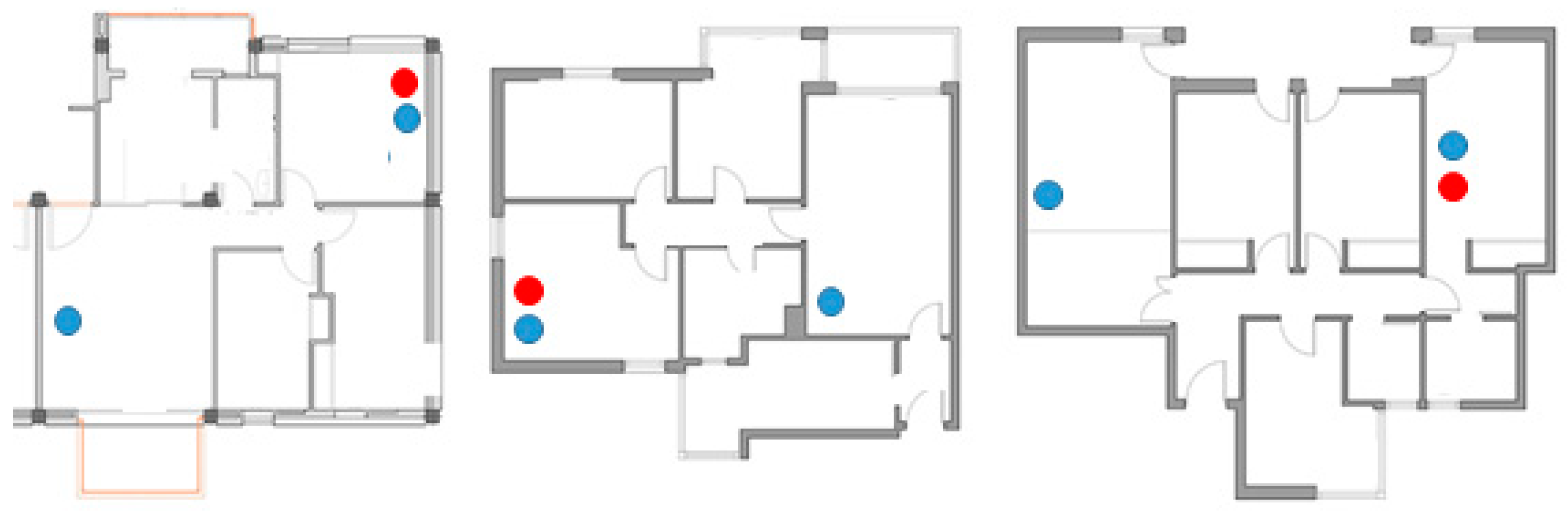
This paper aims to analyze the indoor air quality (CO2, TVOC, and PM2.5) in three representative case studies in Andalusia, in order to establish whether there is a correlation between indoor air quality and different parameters or occupant behavior.

2. Materials and Methods

2.1. Context and Location

Seville is a city in the south of Spain with the largest housing stock, of which more than one third can be classified as social type and over half was built before 1979 [9]. The population of the city is about 700,000, although considering the floating population, and the metropolitan area this figure exceeds 1,500,000 inhabitants [47], hence its special representativeness and impact. Located at latitude 37˚25´ N and at a height of 26 meters, this city [48] has a temperate climate with an annual average temperature of 18.6°C. Although, in general, the winters are mild with minimum average temperatures of 5 °C, the cold period may generate discomfort and inadequate indoor conditions —even temperature related health-issues— in low-standard housing [49]. Summers are hot and dry with peak temperatures reached from May to September, usually with broad daily thermal oscillation [50]. The midseason is long, with many hours of mild temperatures throughout the year. This climatic context promotes the use of natural ventilation and the half-open dwelling state for a considerable number of hours per year. This situation makes the area significant as a model for behavior analysis in the building stock, sharing many characteristics with other urban areas in the south of Europe. The traffic levels in the city can be considered high although they do not reach the levels of traffic of large European cities.

2.2. Sampling

The buildings studied were selected after a lengthy process designed to suitably represent the building stock. The first phase identified and characterized 250 social housing developments built within the city limits in the period studied (1940–1979). This totalled 99,437 of an expected total of 100,510 units: in other words 98.93% of the entire population, which for all practical purposes can be regarded as the whole. The procedure for identifying and classifying these units is described in [6].
Subsequent analysis led to grouping the developments into particularly representative types characterized by the features found in each sub-period. A second grouping (covering 83 developments and 46,476 units, or 47% of the population) established the essential morpho-constructional features of these developments, identifying subject types by sub-period and building a matrix of typical characteristics also by sub-period, all of which are described in [9]. Inductive analysis was used to define the population parameters by intervals.
Temperature, humidity, and Carbon dioxide (CO2) level measurements were analyzed for 16 social housing units [18]. In addition, air tightness tests were conducted on the units [13,15] and relationships between this parameter and CO2 concentration were analyzed in this study. A review of the state of the art of this topic suggested that additional parameters such as PM2.5 and VOC should be studied to determine whether indoor CO2 concentration could be used as an indicator of indoor air quality, as shown in other studies. Due to the limited availability of measuring equipment, of the 16 units monitored for CO2, three dwellings representative of different degrees of airtightness and different user behavior were chosen for the study. It represents 3 very common dwelling types in the area —representing extreme and average values airtightness and representative of the social housing stock. They were monitored under normal operative conditions (Table 1).

2.3. Data Collection

Data were collected from July 2017 to June 2018. Daily data were recorded at 10-minute intervals. Instrumentation and methods were monitored following the ISO7726:2002 specifications [51]. This monitoring was conducted in occupied flats. Data were recorded using three sensor sets per unit: one located in the living-room (day zone) and two in the bedroom (night zone) (Figure 1). The CO2 loggers were calibrated by the research group, and the TVOC and PM logger were factory calibrated and provided sufficient accuracy [52]. A Wöhler CDL 210 datalogger recorded the air temperature and relative humidity with an accuracy of 0.5 °C and 3%, respectively, and measured CO2 over a range of 0–9000 ppm, with an accuracy of 50 ppm ±5%. A Foobot datalogger recorded the PM2.5 and TVOC with an accuracy of 4 µg/m3 and 5 %, respectively. Data were downloaded every month in situ.
As indoor CO2 concentration, temperature, and Relative Humidity (RH) are never the same throughout a room [53], the sensor was positioned to detect a mean value, i.e., in the area where occupants would be breathing. That is, between 1 and 1.5 meters high on the living room, and on the bedside table on bedrooms.
Outdoor conditions (outdoor dry air temperature, relative humidity, dew point, wind, and others) were provided by the Spanish National Meteorological Office (AEMET), while the conditions of outdoor PM2.5 distribution and TVOC were obtained from the Consejería de Medio Ambiente y Ordenación del Territorio of the Regional Andalusian Government. Periodic contrast measures were taken using portable reference sensors to ensure consistent and accurate measurements.

2.4. Threshold Level

The limit values, tolerance margins, and warning thresholds for concentrations in ambient air are intended to provide guidance on how to reduce the effects of air pollution on health.

2.4.1. CO2 Concentration

Although the main source of emission for carbon dioxide (CO2) is usually the building occupants, it should be noted that open combustion elements such as gas stoves and Domestic hot water (DHW) heaters — and their combustion gases — are often found within these dwellings. Many indoor air quality (IAQ) studies adopt CO2 concentration as an indicator of actual ventilation rates and as IAQ-index. It is generally accepted that CO2 keeps ‘bad company’ and that levels above 1000 ppm are indicative of poor ventilation rates [54]—which corresponds to a ventilation rate of 8 l/s per person. This standard continues to be relevant, with a threshold referenced in many national and international guidelines [55], which will be the reference value adopted in this work. Even though carbon dioxide is not normally considered an indoor air pollutant, some adverse health effects have been associated with room levels above 5000 ppm due to the displacement of oxygen in the air [56].

2.4.2. PM2.5 Concentration

Airborne particulates are solid or liquid substances suspended in the air flow, and can include dust, fumes, smoke, microorganisms, mist, and fog [57]. These particles can range widely in diameter, the most harmful in domestic environment are respirable suspended particulates (RSPs), especially the fine inhalable particle fraction, 2.5 μm or smaller—PM2.5 [58,59,60,61]. The figures used as the control limit for the analysis proposed will be based on those established by the World Health Organization (WHO) [62], which proposes an annual limit of the concentration of PM2.5 of 10 µg/m3 and a daily limit of 25 µg/m3. Reference values inside dwellings were documented by Gotschi [63], with the lowest concentration (9.5 μg/m3) measured in Finland, and the highest (50 μg/m3) in Italy.

2.4.3. TVOCs Concentration

Together, with the aforementioned, the most common fraction of pollutants within homes is the volatile carbon compound family (VOCs). While there may be thousands of chemicals within this group, almost 900 of them have been identified in the indoor environment, mainly linked to indoor furnishings, finishes, and other building elements such as paint, solvents, adhesives, carpets, fabrics, and textiles. Exposure to elevated airborne concentrations of VOCs can lead to a range of toxicological effects, including fatigue, headaches, drowsiness, and eye irritation among many others [64], both in the short and long term [65]. However, the wide variety of potential sources and compositions renders it impractical to measure the concentrations of each chemical individually. Accordingly, the concept of total volatile organic compound (TVOC) attempts to address this practical limitation by providing a simple measurement for the aggregate of all volatile organic compounds without making distinctions between individual chemicals.
Typically, the concentrations of VOC detected indoors are higher than outdoors and have increased over the past decade, so that outdoor contribution may be considered negligible most of the time. Although there is no common regulation on the admissible TVOCs exposure inside homes, it is possible to establish some general thresholds from which inhabitants’ sensitivity may arise (physiological responses and pathological processes can be identified in occupants). In the range of 120 to 1200 ppb, symptoms of irritation and discomfort can begin to appear in some occupants. Up to 10,000 ppb, these symptoms are generalized, taking different forms depending on the degree of sensitivity of the inhabitants and the species present, developing toxicity levels of up to 10,000 ppb [66]. A maximum level of 120 ppb is usually recommended for the indoor environment to be considered healthy [67]. We have considered this figure a desirable target and figures up to 1200 ppb as a potential-risk indoor environment. These considerations require a general approach and are highly sensitive to the types of VOC compound present, some of which will be very harmful in very low concentrations.

3. Results

3.1. CO2

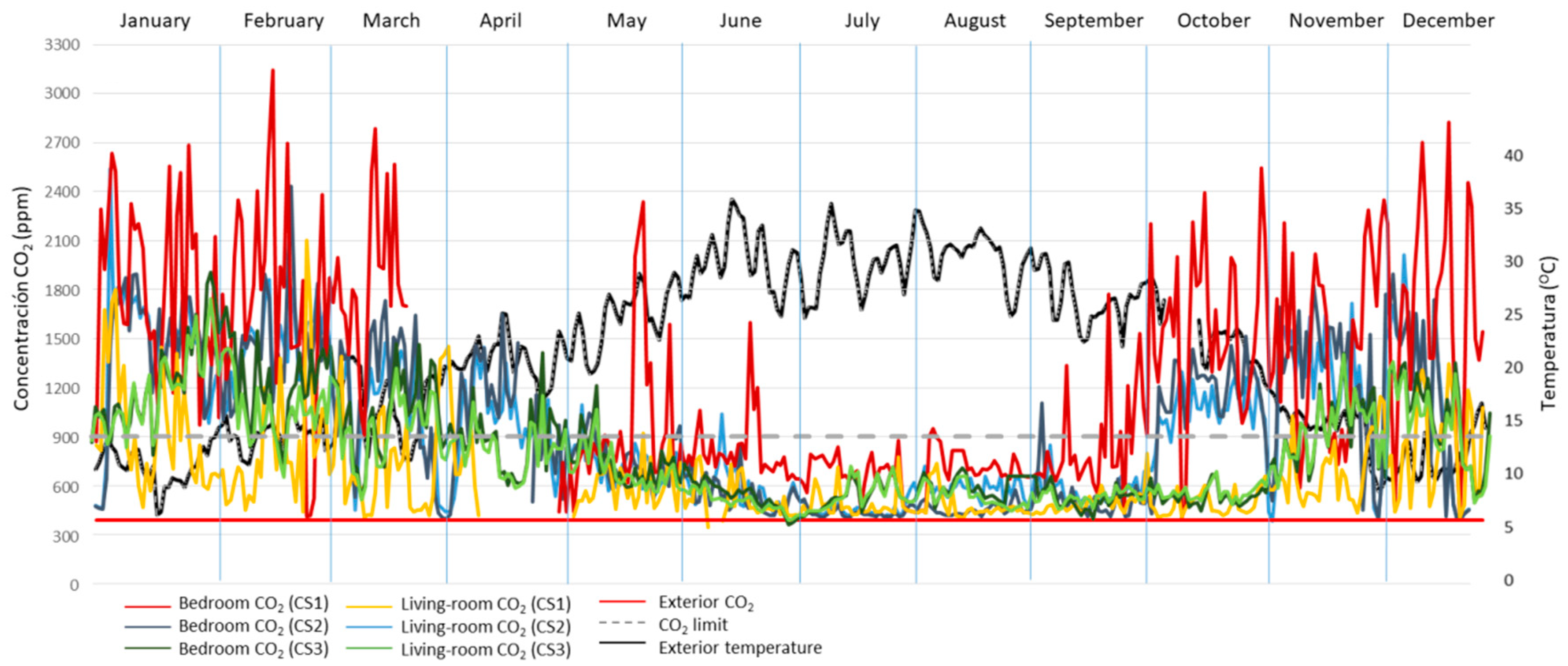
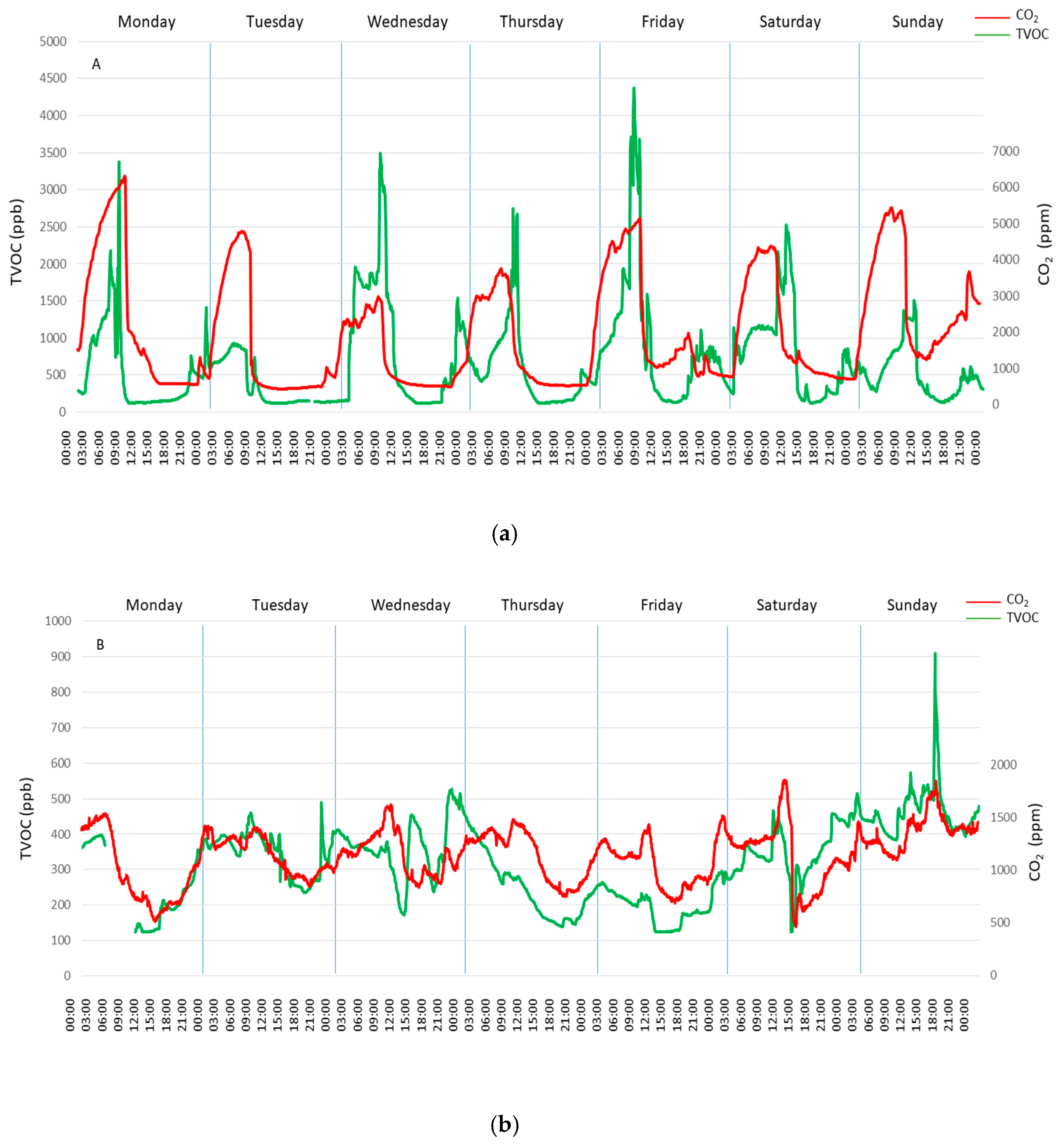
In all three cases, CO2 concentrations have shown wide fluctuations over time. Winter concentrations oscillate between minimums around 400 ppm (barely equivalent to outdoor concentration) and maximums above 2000 ppm. There are some peaks above 4500 ppm in the living rooms and concentrations above 3000 ppm, with peaks above 7500 ppm, in the bedrooms. Typical value (median) for daytime living rooms ranged between 853 ppm (CS1) and 882 ppm (CS2), while for bedrooms this varied between 1199 (CS2) and 2385 ppm (CS1), mostly at night (Figure 2).
CO2 concentration in winter usually exceeds WHO recommendations—a limit value of 1000 ppm for healthy environments [68]—indicating low ventilation rates and a potential risk of air-quality related issues. This aspect is of great significance in bedrooms with conditions below the threshold no more than 50% of the time, (which really corresponds to unoccupied daytime). Even living rooms usually have high figures for several hours (lower values for CS1 may be attributed to low use intensity due to work schedules).
There is a clear relationship between infiltration and CO2 concentration values, stronger in bedrooms at night. The least airtight dwelling (CS3) remains below 1000 ppm more often (for a similar emission source of two people during sleep time) than the two more airtight dwellings.
In mild season conditions, the frequent operation of windows in a semi-open situation for extended periods allows CO2 concentration to fall below 1000 ppm in living rooms most of the time, between 95% and 99% of the hours. Although the values in the bedrooms are much lower than in winter, they present a wider distribution. Users often close windows at night, increasing CO2 concentrations, with 10% to 20% of the hours over the 1000 ppm line (Figure 3).
There is a clear indoor state shift between the cold season and the intermediate one in terms of quality if carbon dioxide is assumed as IAQ indicator. This is clearly related to the evolution from closed environment to the semi-open model.
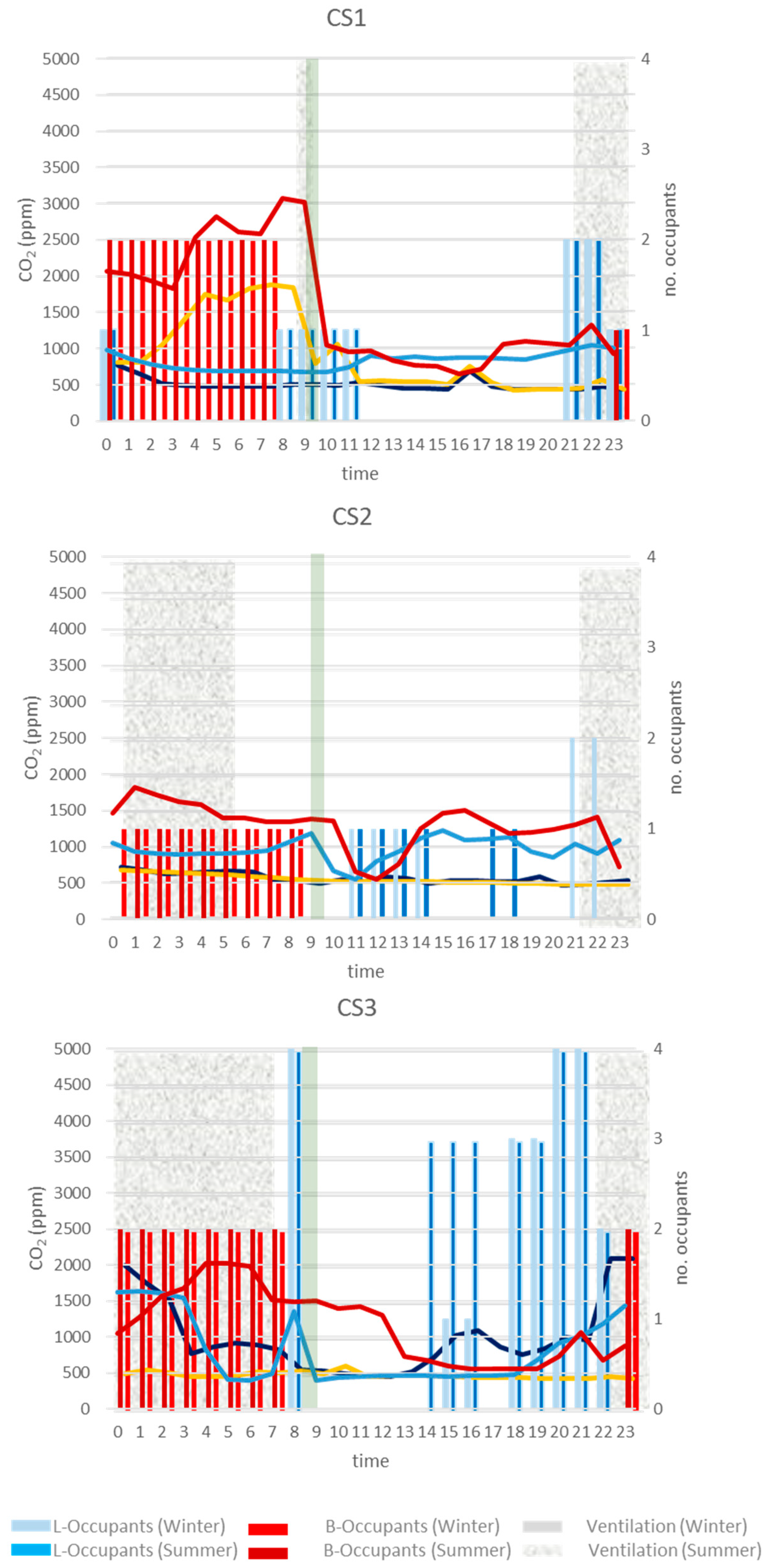
Hours of occupancy in bedrooms and living rooms and the number of occupants in each, along with reported ventilation times, are shown in Figure 4. CO2 concentration by time of day is also presented in the figure in order to determine whether users’ replies to the surveys were consistent with CO2 analysis.
Hours of occupancy and number of occupants reported varied widely. In winter, Seville dwellings were ventilated for 10 to 30 min in the morning. In contrast, in summer, windows remained open all night in CS2 and CS3.
In CS2, the number of occupants tended to be small, as the users were not usually present at the same time. This dwelling also had the lowest CO2 concentration.

3.2. Particle Concentration (PM2.5)

During measurement, PM2.5 indoor concentrations present a wide oscillation without a clear pattern. Annual average values are 16.09 μg/m3 (CS1), 7.1 μg/m3 (CS2), and 9.66 μg/m3 (CS3). CS1 exceeds the annual limit for the concentration of PM2.5 of 10 µg/m3. Although dwelling CS1 presents strong peaks, it is not representative of the average internal situation. The dwelling ambient reaches values as high as 1402 μg/m3 although normal values usually remain below 50 μg/m3 (95th percentile representation). Even so, these values are high in relation to the recommendations of the WHO [68] and the European Environmental Agency (EEA) [69]. During winter, the less airtight dwelling tends to have higher median PM2.5 concentrations (95th percentile = 25.14 μg/m3) (Table 2). Users exceed the PM2.5 threshold of 10 µg/m3 between 45% and 15% of the hours (Figure 5).
In all three cases, the PM2.5 daily average reference value is not exceeded, except for peak episodes of particles of indoor origin in dwelling CS1 during the winter. However, the usual values are relatively high (Table 3).
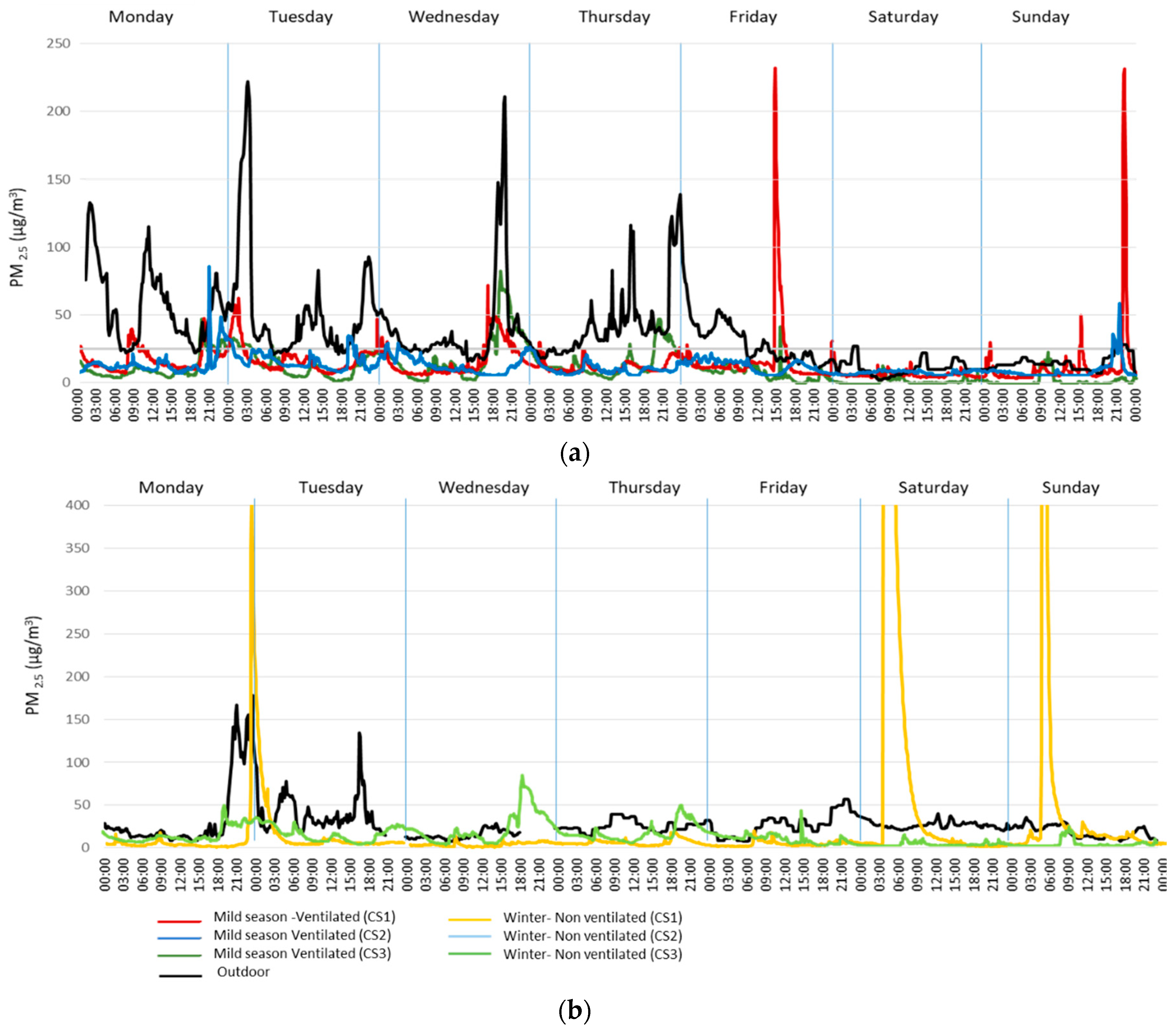
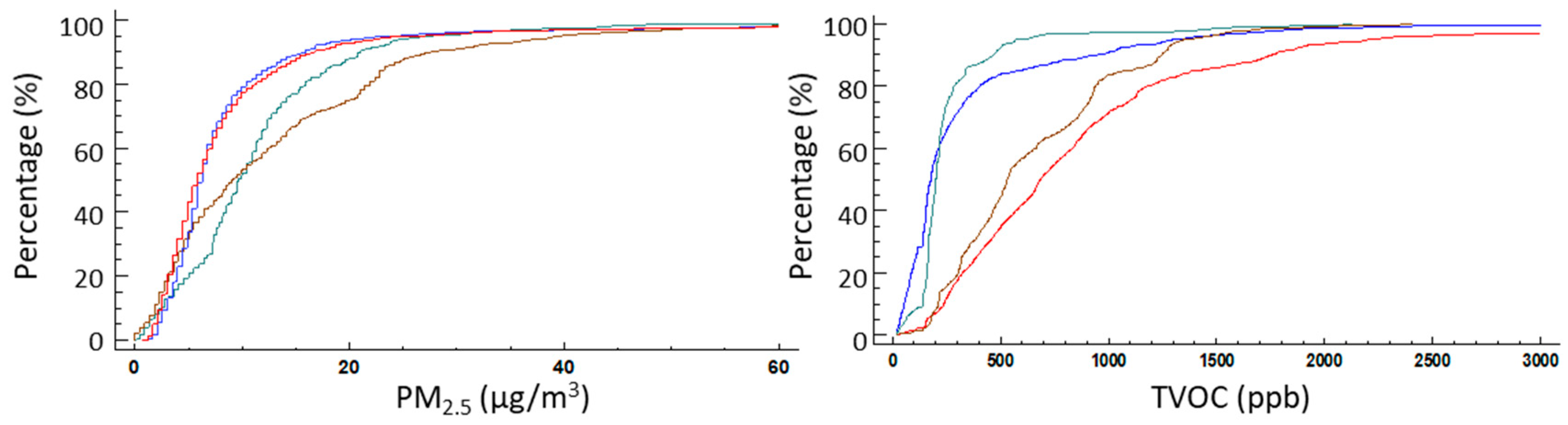
In the mild season typical week (Figure 6a), the outdoor mean values are much higher than those measured indoors, although there are some indoor peaks over 230 µg/m3. Apart from the semi-open situation of the dwellings, there is no clear response pattern to outdoor evolution. This effect may be due to users’ habit of maximizing ventilation during night time, when outdoor concentrations are usually lower, while the windows remain closed for most of the day. The lower peaks are found in dwelling CS2 with 78 µg/m3, followed by CS3 with 82 µg/m3. CS1 displays a slightly different behavior from the previous two cases. Although the outdoor–indoor differential is still high, there is a clearer relationship in the evolution of both atmospheres: late in the afternoon, the indoor PM2.5 values reflect the evolution of the outdoor conditions, with a significant decrease. In this time interval, the higher frequency in the opening of windows is noted and this is when peaks are identified.
However, during the winter (Figure 6b), a decoupling of both indoor and outdoor PM2.5 concentration evolutions occurs, primarily through the open-window time reduction, with homes remaining closed most of the time. In CS1, peaks of indoor concentrations appear to be generated endogenously with no connection to the outside atmosphere, where 200 µg/m3 is not usually exceeded.
Figure 7 shows the time distribution of PM2.5 concentration in a typical week in winter and mild season. The dispersion of the measured values observed in CS1 is greater between 15 and 17 h, a time slot in which the inhabitants of this home usually cook—the dwelling does not have mechanical extraction in the kitchen. In CS2 and CS3, the higher ranges of value dispersion match the ventilation schedules of the dwellings.

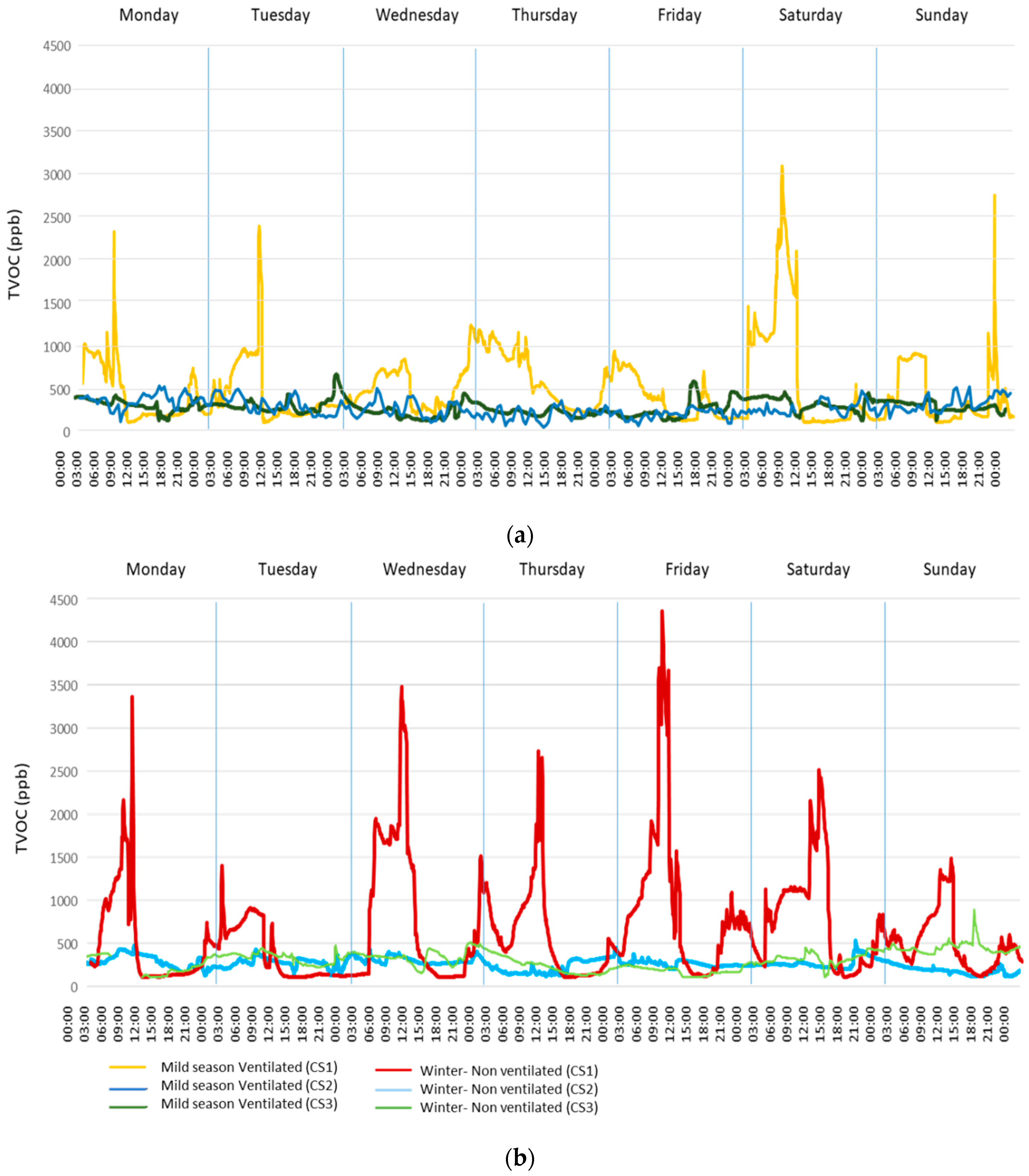
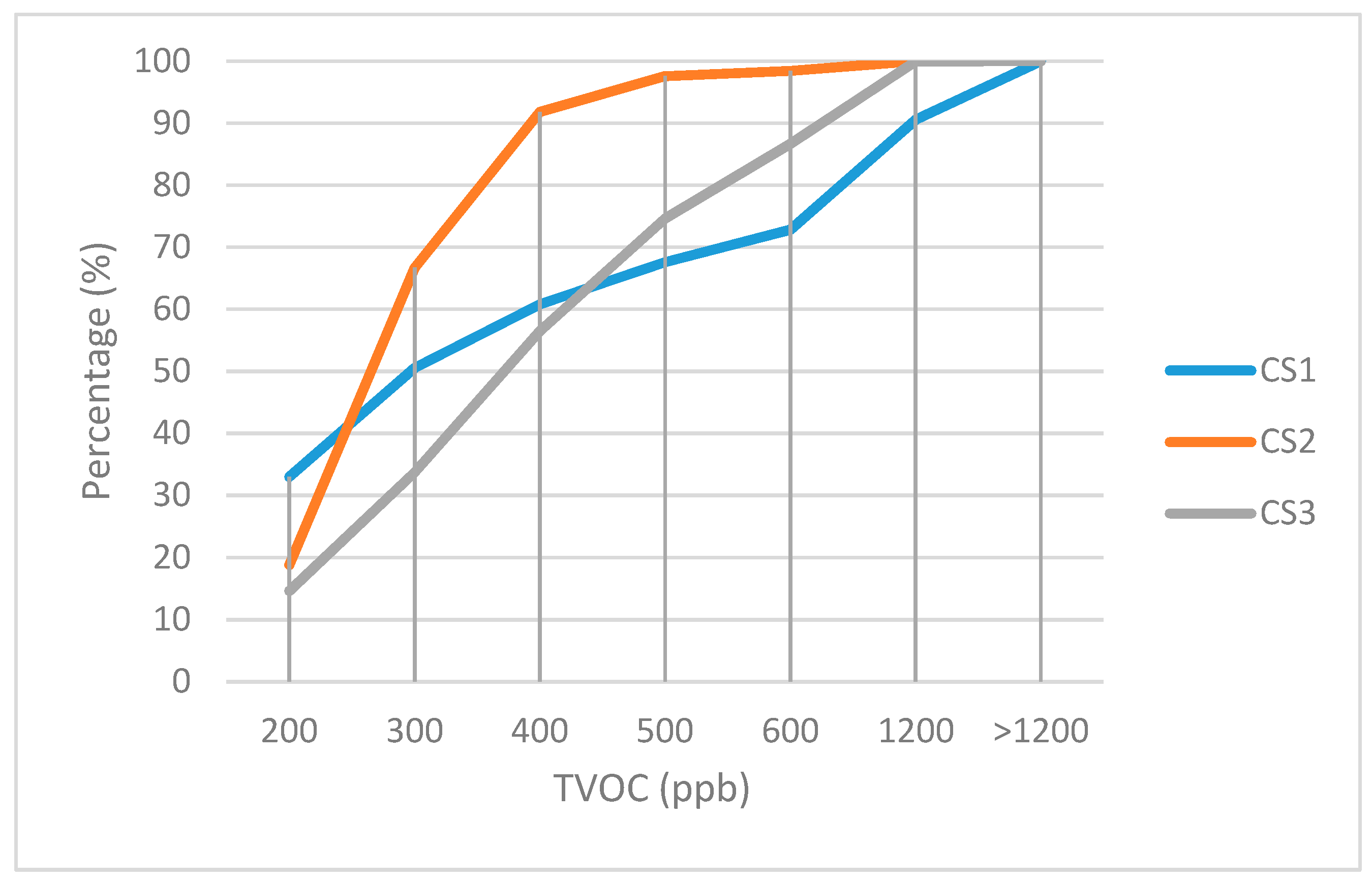
3.3. TVOC Concentration

A concentration limit of <120 ppb was adopted as a healthy environment reference and a threshold over 1200 for risk environment. These considerations are a general rule but are very variable depending on the type of VOC compound present in the atmosphere. The presence of VOCs is due primarily to emissions of domestic origin. Inhabitants’ presence has a special repercussion, as has the type of activities performed. The movement of occupants increases the effect of internal ambient turbulence by increasing the effect of the mixture of pollutants. There is also a significant contribution from indoor construction materials, generating a near continuous base level of VOCs, but the greatest effect can be linked to the use of chemicals in daily housework and personal care. The external contribution of VOCs is unusual. Therefore, the outdoor environment external action—through ventilation or building envelope air permeability—is noted in the dilution effect on indoor VOCs.
Indoor average TVOC concentration is usually below the 1200 ppb threshold with uneven distribution: the 95th percentile values are 1698 ppb (CS1), 420 ppb (CS2), and 672 ppb (CS3), with no regular behavior patterns. The indoor concentrations are higher in winter than in summer: in summer, more frequent opening of windows contributes to greater dilution. There are high concentration peaks in CS1, all below the toxicity threshold of 10,000 ppb. These environments cannot be defined as healthy and VOC-free environments except in specific periods, when they remain outside the most dangerous exposure levels (Figure 8, Figure 9, and Table 4).
Globally, the more airtight dwellings have higher TVOC concentrations, although this parameter is distorted by the different emission rates in individual dwellings, which makes it difficult to identify this factor positively.
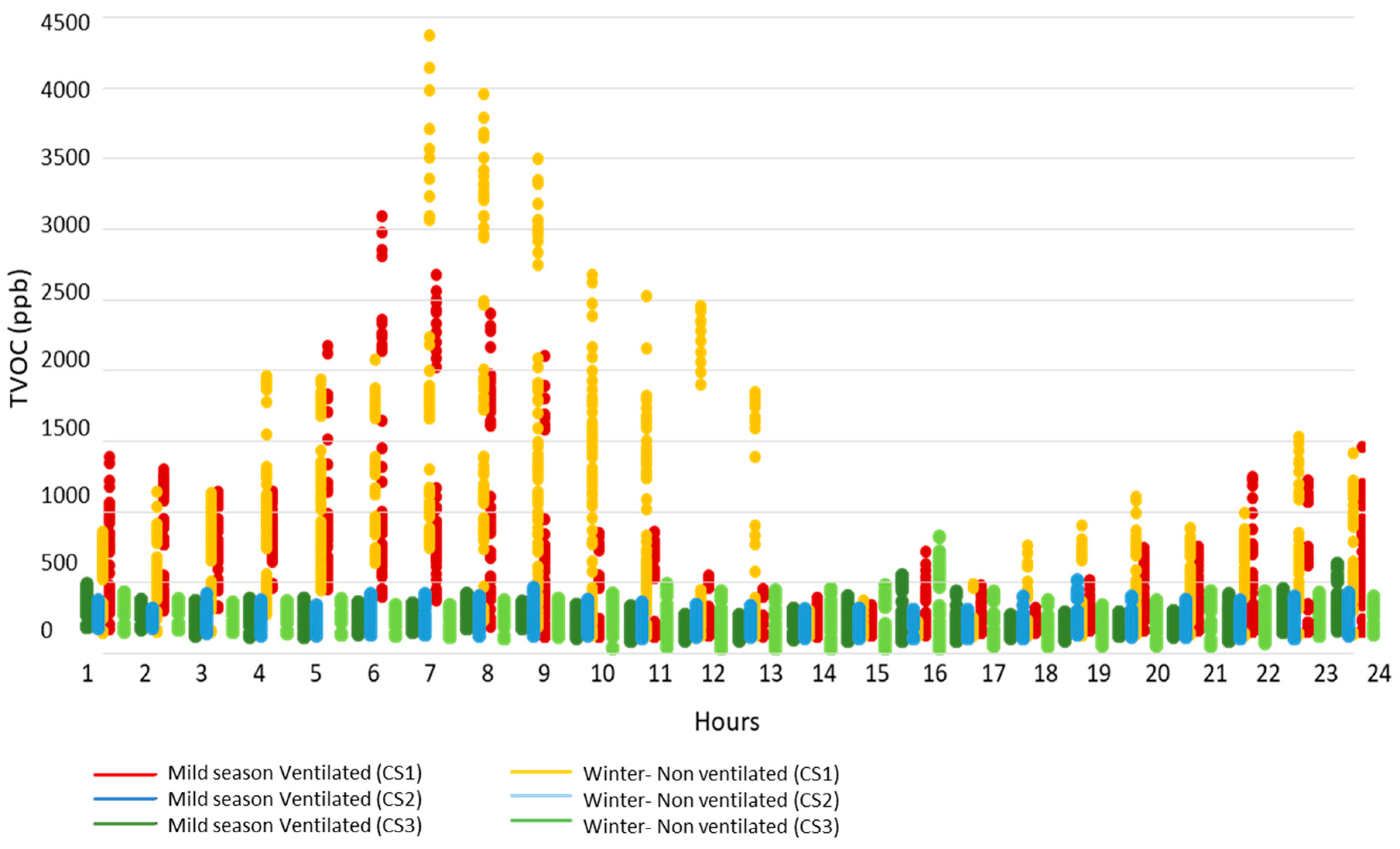
Figure 10 shows the time dispersion of TVOC concentration in a week in winter and mid-season. In CS1, values are well above those recorded in the other two case studies. The highest values are reached in winter, when the dwellings are not ventilated. The maximum peaks match periods when some personal care products, such as deodorants or hairsprays, are used by residents. In CS2, these figures are small and distributed over time, indicating that activities carried out by the occupants of these homes tend not to generate this kind of pollutant and housing is ventilated frequently through the vent opening windows. A uniform distribution in time is observed with maximum values reached about 4 pm, in CS3 slightly more than in CS2, coinciding with the time of cooking.
These results are consistent with the habits of the users. In CS1, the users, a couple, spend much of the day practicing hobbies such as miniature paintings or using sprays or makeup products. In CS2, also inhabited by a couple, the interests are movies, reading, or playing the guitar. As a result, less TVOC production is derived from CS2 than from CS1. Finally, CS3 with four inhabitants, two of them children, shows TVOC values between the previous two.
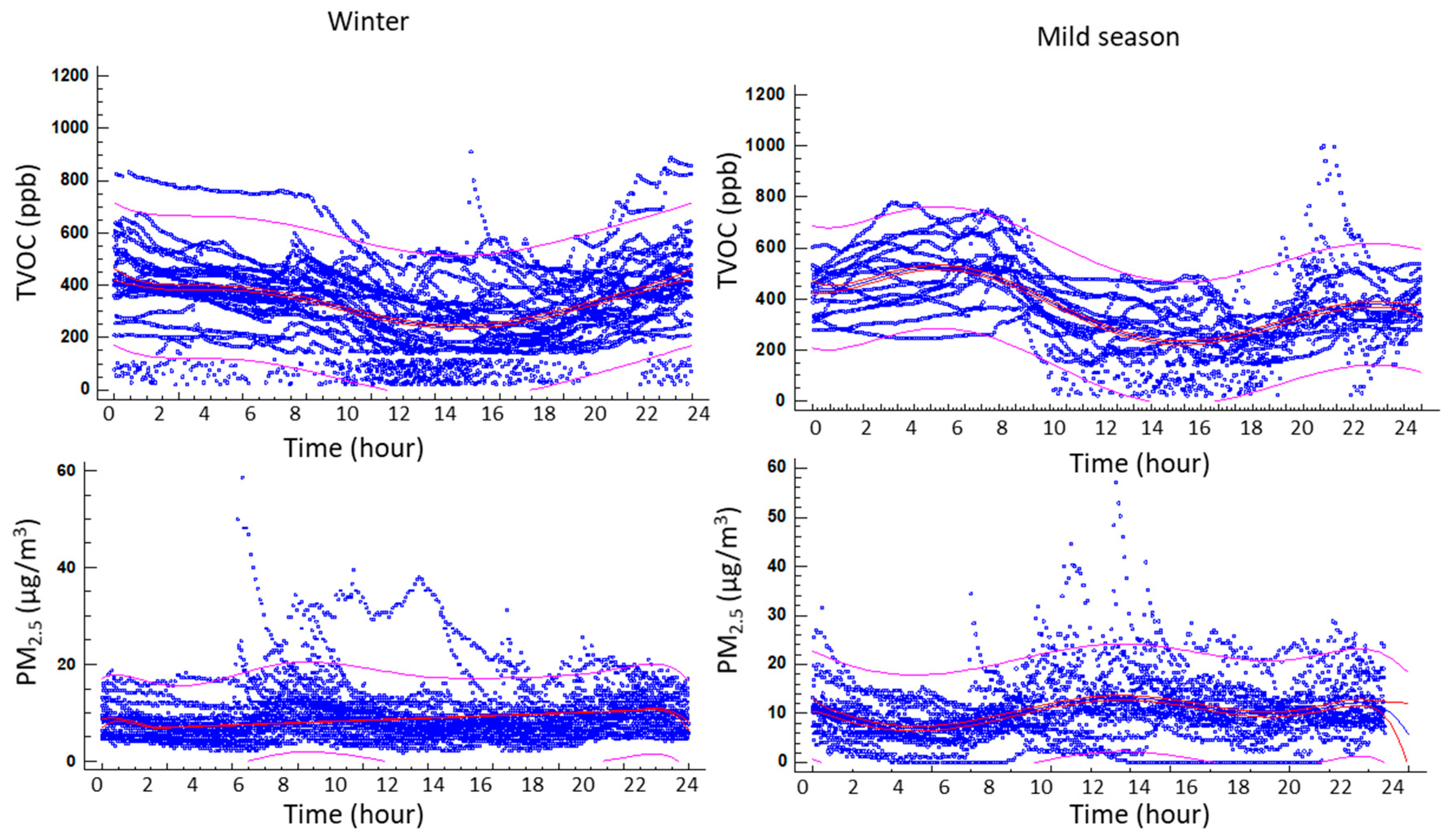
4. Discussion

The dwellings analyzed tend to show very different behaviors between cold and mild-warm periods. During cold weather periods, daily window operation is restricted to short periods, which results in two different indoor/outdoor environments (closed-house) where air interchange is mostly dependent on envelope airtightness. During mild seasons, building enclosure permeability increases due to the opening of the windows, often with a significant proportion of the windows staying open for most of the day, in this case a semi-open indoor environment is developed in the home.
Although parameter variability is high, given the stochastic nature of the parameters associated with external phenomena and use, it does not allow an expected hourly value to be established accurately, a tendency which is further supported by previous analysis. The evolution of concentrations is more stable in winter, since dwelling windows remain closed most of the time, slowing down the air-exchanges (Figure 11).
VOCs and PM2.5 show opposite evolution patterns and a relationship, albeit a rather limited one, can be established in the middle of the day, when most of the ventilation occurs. This can be identified by the presence of the highest daily particle penetration, with the house remaining closed the rest of the time [70,71,72,73,74]. However, the particle presence is constant, significant enough, but with lower values. Despite internal production of VOCs, this can be attributed to envelope penetration, which is in turn responsible for the dilution of VOCs observed (for example, at dawn with inflections visible from minute 300).
Particularly in the mild season, the daily variation is more pronounced, with a clear difference between night and day as the windows are kept open longer in the middle part of the day. Indoor species are much diluted in the daytime but rise at night. Particle penetration daily-shift is less noticeable, increasing slightly in the central part of the day but remaining stable for the rest of the day. It should be noted that the particle penetration peaks at morning (around 8:00 am, minute 480) and this can be associated with initial ventilation. There is a secondary trend change at around 9:30 p.m. when this ventilation is usually increased and the windows are fully opened to dissipate the indoor daily accumulated thermal-loads of homes, moderating the VOCs at the same time. ANOVA tests were carried out to identify whether cold and midseason PM concentration datasets are related to the same probabilistic distribution (representing the same actual behavior) or whether the difference between seasons is of enough statistical significance to allow an actual pattern difference between seasons to be assumed. The F-ratio was found to be equal to 1286.31 in VOC concentration and 2072.88 in PM2.5. Since the P-value of the F-test is below 0.05 in both cases, there is a statistically significant difference between the means of the 2 variables with a 95.0% level of confidence (Figure 12).
The period when dwellings are mostly closed shows the greatest indications of pollutant evolution (Figure 13). Assuming that most of the homes lack adequate thermal systems so that effective thermal control is not possible, the homes show a close relationship between external temperature drop and ventilation rate decrease, resulting in a lower ventilation driven dilution. This situation is clearly highlighted by the correlations between indoor related parameters (CO2, VOC, and RH) and the outdoor evolution of temperature. The most obvious case is the positive correlation (0.50) between CO2 indoor-concentration and the outdoor–indoor temperature difference (ΔT), similar to outdoor air-temperature (–0.46), which is negative in this case. These relationships would be highlighted if unoccupied periods were excluded (Figure 13).
Indoor parameters show a significant cross-relationship between humidity and VOCs, which may be associated to indoor home activity. The weaker CO2 dependency shows a closer link to specific task emissions, especially those related to activities in the kitchen and bathroom, than to normal inhabitant presence.
Cold season, even in mild climate areas, shows indoor environments isolated from the exterior much of the time, with no linear link to the outdoor air quality daily evolution beyond external temperature inverse ventilation rate dependency leading to worse indoor air-quality parameters. The stronger probabilistic parameter is external temperature, with a clear inverse dependency with natural ventilation. Natural ventilation rate shows a clear inverse-dependency to outdoor temperature and thus indoor air quality indicators (Table 5).
In the mild season, the relationship between indoor/outdoor environments is strengthened and becomes clearly dependent (outdoor > indoor) (Table 6). This can be seen in the downward shift of the concentration pattern of indoor-origin pollutants due to a greater ventilation-driven dilution, and also to the indoor mirroring of outdoor thermal oscillations. Humidity and air temperature evolution couple with outside conditions with little to no thermal decrease and time lag due to the high air interchange rate. However, indoor species show specific dynamics with slight correlations between the parameters relating to the pollutants. This does not apply to RH and indoor-air temperature, which are mostly collinear. However, interior species characterized by very specific dynamics differ greatly and are much more unique than those in winter. Only weak correlations are found between indoor physical parameters and pollutant concentration.
It should be noted that despite the expected colinearity between PM2.5iIND-PM2.5OUT, this is somewhat weak (0.37) and slightly distorted, indicating the presence of different mechanisms of particle distribution and indoor-capture, including those relating to indoor emissions (internal sources of particle emission) and those linked to infiltration through the envelope and surface absorption of particulate matter in the indoor environment.
While some of the peak episodes can be understood as unique, they represent potential stages within households where high figures are often present due to internal activity. These cases can be understood as beacons of current trends, identifying a transition to an indoor-source scenario. This trend has also been identified in the literature, linked to the increasing use of furniture made of synthetic materials, as well as to the growing tendency to use chemicals at home for both cleaning and personal care [55,56,57,58,59].

5. Conclusions

The parameters that define IAQ in the indoor environment in the dwellings under survey show figures far from those generally accepted as healthy for most of the year. This situation results in the overall excessive exposure of home inhabitants. However, these figures vary greatly, due mainly to the variable occupancy pattern in the dwelling and the relationship with window opening response.
Indoor CO2 concentrations clearly correlate with airtightness but typically exceed the 1000 ppm limit recommended by the WHO for healthy environments in all cases.
Indoor particle (PM2.5) levels are highly variable. This parameter is strongly related to outdoor conditions, so no regular pattern can be established. Indoor levels are relatively high when dwellings are in a half-open situation in the mild season and periods in which the windows usually remain open due to weather and urban environment conditions. During cold periods, the less airtight flats usually present the highest PM2.5 particle concentration figures. Otherwise, the most airtight properties usually show higher TVOC concentrations, although this parameter is highly distorted by the irregular patterns of indoor-source emission rates linked to indoor activities. In winter, most of the time, these usually remain below the recommended threshold of 1200 ppb, when the effects of TVOCs are usually noticed. However, peak episodes above these limits are not unusual in the homes analyzed, but they remain under the toxicity threshold of 10,000 ppb.
Although these homes cannot be considered actual healthy environments in long-term exposure, they do not reach potentially hazardous short-term exposure situations, except for short time-frames.
The building interface system (envelope and windows) of these dwellings is no longer able to guarantee adequate indoor environments for a significant number of hours per year, even in locations traditionally identified as lightly-polluted environments, such as those of southern Spain.
The current approach for housing energy retrofitting relies heavily on the addition of insulation layers to the fabric, new airtight windows, and air-seal enhancement of joints. The current ability of dwelling stock to incorporate mechanical ventilation and thermal appliances into these dwellings, as promoted by some strategies such as Passivhaus, is very limited and is restricted by factors such as interval height or lack of technical spaces. Consequently, the disruption of the air-interchange dynamics resulting from increasing air-tightness and supported by the progressive change in lifestyle can become a growing risk-factor for inhabitants’ health, even in regions where traditionally the opening of windows has been fully established.
A final question arises: Do current energy conservation approaches lead to scenarios where the health of the indoor environment is put at risk? As has been emphasized, current air-exchange rates must be increased for a better indoor dilution and removal of pollutants, something which is difficult to achieve in the absence of mechanical ventilation systems. This also contradicts the usual techniques of improving the energy conservation approach, mainly based on increasing thermal resistance and airtightness, as these measures become less effective as a significant portion of the total energy transfer is linked to the interchange of air masses. Therefore, there is a need for further research and discussion to identify the appropriate rates of air-exchange for contemporary stock-dwellings and how these could be made compatible with energy saving needs.
Whole-house mechanical ventilation, such as that required by ASHRAE Standard 62.2, has proven to be an effective strategy for some contaminants. In keeping with this assumption, higher levels of ventilation air have been shown to reduce concentrations of many VOCs. However, this measure is difficult to follow in the housing stock in need of retrofitting.
Despite the difficulty, it would be advisable for further research to focus on identifying good practice in ventilation and the optimization of envelope airtightness. This would serve as a basic step for the development of specific guides, with the potential for specialization by building type and features [75,76,77]. These could provide tailored ventilation protocols and calendars which would allow users to modify their current customs, which are often counterproductive to maintaining good conditions. In addition, it would also make it possible to work on airtightness to ensure optimum conditions are obtained, especially when working on retrofits. This would prevent instances of insufficient ventilation in spaces, as long as no mechanical ventilation systems were installed. However, the implementation of this measure as a widespread solution is unlikely at present. Finally, this would also allow the development of information systems, via APPs or personal devices, to adapt ventilation needs and their integration with new control domotics systems and If This Then That (IFTTT )protocols for instance.

Author Contributions

Conceptualization, J.F.-A. and S.D.-A.; Data curation, J.F.-A. and S.D.-A.; Formal analysis, J.F.-A., S.D.-A., M.F.and F.O.; Investigation, J.F.-A. and S.D.-A.; Methodology, J.F.-A., S.D.-A., M.F.and F.O.; Supervision, J.F.-A.; Writing–original draft, J.F.-A., S.D.-A., M.F.and F.O.; Writing–review & editing, J.F.-A., S.D.-A., M.F.and F.O.

Funding

This research received no external funding.

Acknowledgments

The wind velocity and outdoor temperature data were furnished by Spain’s National Meteorology Agency (AEMET), and outdoor PM2.5 distribution and TVOC´s by the Consejeria de Medio Ambiente y Ordenación del Territorio of the Regional Andalusian Government. The authors wish to thank to Dipartimento di Ingegneria Civile ed Ambientale, Università degli Studi di Perugia for their welcome in the authors research stay.

Conflicts of Interest

The authors declare no conflict of interest.

References

  1. Sendra, J.J.; Domínguez-Amarillo, S.; Bustamante, P.; León, A.L. Energy intervention in the residential sector in the south of spain: Current challenges. Inf. Constr. 2013, 65, 457–464. [Google Scholar] [CrossRef]
  2. Fernández-Agüera, J.; Sendra Salas, J.J.; Suárez Medina, R.; Domínguez-Amarillo, S. Airtightness and Indoor Air Quality in Subsidised Housing in Spain. In Proceedings of the 36th AIVC Conference, Madrid, Spain, 23–24 September 2015. [Google Scholar]
  3. Domínguez, S.; Sendra, J.J.; León, A.L.; Esquivias, P.M. Towards Energy Demand Reduction in Social Housing Buildings: Envelope System Optimization Strategies. Energies 2012, 5, 2263–2287. [Google Scholar] [CrossRef] [Green Version]
  4. Eurostat. Living Conditions in Europe; European Union: Luxembourg, 2014; p. 1. [Google Scholar]
  5. Pennestrì, D. The energy and Enviromental requalification of post-war housing: Problematics and innovative solutions for the building envelope. In Central Europe Towards Sustainable Buildings 2013: Sustainable Refurbishment of Existing Building Stock; CESB13: Prague, the Czech Republic, 2013; pp. 1–7. Available online: http://www.cesb.cz/cesb13/proceedings/1_refurbishment/CESB13_1243.pdf (accessed on 7 November 2019).
  6. Domínguez-Amarillo, S.; Sendra, J.J.; Fernández-Agüera, J.; Escandón, R. La Construcción de la Vivienda Social en Sevilla y su Catalogación 1939–1979; Universidad de Sevilla: Sevilla, Spain, 2017. [Google Scholar]
  7. Ferrari, S.; Zanotto, V. Building Energy Performance Assessment in Southern Europe; Springer: Milano, Italy, 2015. [Google Scholar]
  8. Matteis, D. Affordable Housing Praxis for Urban Sustainability; Ipertesto. Europen Programme for Urban Sustainable Development: Verona, Italy, 2008. [Google Scholar]
  9. Domínguez-Amarillo, S.; Sendra, J.J.; Oteiza San José, I. La Envolvente Térmica de la Vivienda Social: El Caso de SEVILLA, 1939 a 1979 Title, 1st ed.; Editorial Consejo Superior de Investigaciones Científicas: Madrid, Spain, 2016. [Google Scholar]
  10. Allen, J.; Barlow, J.; Leal, J.; Maloutas, T.; Padovani, L. Housing and Welfare in Southern Europe; Blackwell Publishing Ltd: Hoboken, NJ, USA, 2008. [Google Scholar]
  11. BPIE. Europe’s Buildings under the Microscope; European Union: Bruxelles, Belgium, 2011. [Google Scholar]
  12. Código Técnico de la Edificación (CTE); Real Decreto 314/2006 de 17 de marzo: Madrid, Spain, 2006; Volume BOE 74 Ministerio de vivienda, pp. 1816–11831.
  13. Fernández-Agüera, J.; Domínguez-Amarillo, S.; Sendra, J.J.; Suárez, R. An approach to modelling envelope airtightness in multi-family social housing in Mediterranean Europe based on the situation in Spain. Energy Build. 2016, 128, 236–253. [Google Scholar] [CrossRef]
  14. Fernández-Agüera, J.; Sendra, J.J.; Domínguez, S.; Domínguez-Amarillo, S. Protocols for measuring the airtightness of multi-dwelling units in Southern Europe. Procedia Eng. 2011, 21, 98–105. [Google Scholar] [CrossRef]
  15. Fernández-Agüera, J.; Domínguez-Amarillo, S.; Sendra, J.J.; Suárez, R.; Oteiza, I. Social housing airtightness in Southern Europe. Energy Build. 2019, 183, 377–391. [Google Scholar] [CrossRef]
  16. Santamouris, M.; Kolokotsa, D.; Santamouris, M. On the impact of urban overheating and extreme climatic conditions on housing, energy, comfort and environmental quality of vulnerable population in Europe. Energy Build. 2015, 98, 125–133. [Google Scholar] [CrossRef]
  17. Giancola, E.; Soutullo, S.; Olmedo, R.; Heras, M.; Celemin, M.D.R. Evaluating rehabilitation of the social housing envelope: Experimental assessment of thermal indoor improvements during actual operating conditions in dry hot climate, a case study. Energy Build. 2014, 75, 264–271. [Google Scholar] [CrossRef]
  18. Domínguez-Amarillo, S.; Fernández-Agüera, J.; Sendra, J.J.; Roaf, S. Rethinking User Behaviour Comfort Patterns in the South of Spain—What Users Really Do. Sustainability 2018, 10, 4448. [Google Scholar] [CrossRef]
  19. McGill, G.; Oyedele, L.O.; McAllister, K. Case study investigation of indoor air quality in mechanically ventilated and naturally ventilated UK social housing. Int. J. Sustain. Built Environ. 2015, 4, 58–77. [Google Scholar] [CrossRef] [Green Version]
  20. European Commission. Risk Assessment on Inddor Air Quality; Eurpean Union: Brussels, Belgium, 2007. [Google Scholar]
  21. Begum, B.A.; Hopke, P.K. Identification of Sources from Chemical Characterization of Fine Particulate Matter and Assessment of Ambient Air Quality in Dhaka Bangladesh. Aerosol Air Qual. Res. 2018, 19, 118–128. [Google Scholar] [CrossRef]
  22. Kozákovác, J.; Leoni, C.; Klán, M.; Hovorka, J.; Racek, M.; Kostejn, M.; Ondráček, J.; Moravec, P.; Schwarz, J. Chemical Characterization of PM1-2.5 and its Associations with PM1, PM2.5-10 and Meteorology in Urban and Suburban Environments. Aerosol Air Qual. Res. 2018, 18, 1684–1697. [Google Scholar] [CrossRef] [Green Version]
  23. Vormittag, E.M.; Rodrigues, C.G.; De André, P.A.; Saldiva, P.H.N. Assessment and Valuation of Public Health Impacts from Gradual Biodiesel Implementation in the Transport Energy Matrix in Brazil. Aerosol Air Qual. Res. 2018, 18, 2375–2382. [Google Scholar] [CrossRef] [Green Version]
  24. Sarigiannis, D.A.; Kermenidou, M.; Nikolaki, S.; Zikopoulos, D.; Karakitsios, S.P. Mortality and Morbidity Attributed to Aerosol and Gaseous Emissions from Biomass Use for Space Heating. Aerosol Air Qual. Res. 2015, 15, 2496–2507. [Google Scholar] [CrossRef] [Green Version]
  25. Patino, E.D.L.; Siegel, J.A. Indoor environmental quality in social housing: A literature review. Build. Environ. 2018, 131, 231–241. [Google Scholar] [CrossRef]
  26. Vardoulakis, S.; Dimitroulopoulou, C.; Thornes, J.; Lai, K.-M.; Taylor, J.; Myers, I.; Heaviside, C.; Mavrogianni, A.; Shrubsole, C.; Chalabi, Z.; et al. Impact of climate change on the domestic indoor environment and associated health risks in the UK. Environ. Int. 2015, 85, 299–313. [Google Scholar] [CrossRef] [PubMed] [Green Version]
  27. Arvanitis, A.; Kotzias, D.; Kephalopoulos, S.; Carrer, P.; Cavallo, D.; Cesaroni, G.; De Brouwere, K.; de Oliveira-Fernandes, E.; Forastiere, F.; Fossati, S.; et al. The INDEX-PM project: Health risks from exposure to indoor particulate matter. Fresenius Environ. Bull. 2010, 9, 2458–2471. [Google Scholar]
  28. Bari, M.A.; Kindzierski, W.B.; Wheeler, A.J.; Héroux, M.-E.; Wallace, L.A. Source apportionment of indoor and outdoor volatile organic compounds at homes in Edmonton, Canada. Build. Environ. 2015, 90, 114–124. [Google Scholar] [CrossRef]
  29. Jones, A.P. Indoor air quality and health. Atmos. Environ. 1999, 33, 4535–4564. [Google Scholar] [CrossRef]
  30. Deng, Q.; Lu, C.; Ou, C.; Liu, W. Effects of early life exposure to outdoor air pollution and indoor renovation on childhood asthma in China. Build. Environ. 2015, 93, 84–91. [Google Scholar] [CrossRef]
  31. McGill, G.; Qin, M.; Oyedele, L. A case study investigation of indoor air quality in UK Passivhaus dwellings. Energy Procedia 2014, 62, 190–199. [Google Scholar] [CrossRef]
  32. McGill, G.; Oyedele, L.O.; McAllister, K.; Qin, M. Effective indoor air quality for energy-efficient homes: A comparison of UK rating systems. Archit. Sci. Rev. 2016, 59, 159–173. [Google Scholar] [CrossRef]
  33. Vilčeková, S.; Apostoloski, I.; Mečiarová, Ľ.; Burdová, E.; Kiseľák, J. Investigation of Indoor Air Quality in Houses of Macedonia. Int. J. Environ. Res. Public Health 2017, 14, 37. [Google Scholar] [CrossRef] [PubMed]
  34. Mečiarová, Ľ; Vilčeková, S.; Burdová, E.K.; Kiselák, J. Factors Effecting the Total Volatile Organic Compound (TVOC) Concentrations in Slovak Households. Int. J. Environ. Res. Public Health 2017, 14, 1443. [Google Scholar] [Green Version]
  35. Satish, U.; Mendell, M.J.; Shekhar, K.; Hotchi, T.; Sullivan, D.; Streufert, S.; Fisk, W.J. Is CO2 an indoor pollutant? Direct effects of low-to-moderate CO2 concentrations on human decision-making performance. Environ. Health Perspect. 2012, 120, 1671–1677. [Google Scholar] [CrossRef] [PubMed]
  36. Hesaraki, A.; Myhren, J.A.; Holmberg, S. Influence of different ventilation levels on indoor air quality and energy savings: A case study of a single-family house. Sustain. Cities Soc. 2015, 19, 165–172. [Google Scholar] [CrossRef]
  37. Derbez, M.; Berthineau, B.; Cochet, V.; Lethrosne, M.; Pignon, C.; Ribéron, J.; Kirchner, S. Indoor air quality and comfort in seven newly built, energy-efficient houses in France. Build. Environ. 2014, 72, 173–187. [Google Scholar] [CrossRef]
  38. Fernández-Agüera, J.; Domínguez-Amarillo, S.; Alonso, C.; Martín-Consuegra, F.; Domínguez, S. Thermal comfort and indoor air quality in low-income housing in Spain: The influence of airtightness and occupant behaviour. Energy Build. 2019, 199, 102–114. [Google Scholar] [CrossRef]
  39. Fernández-Agüera, J.; Campano, M.Á.; Domínguez-Amarillo, S.; Acosta, I.; Sendra, J.J. CO2 Concentration and Occupants’ Symptoms in Naturally Ventilated Schools in Mediterranean Climate. Buildings 2019, 9, 197. [Google Scholar]
  40. Missia, D.A.; Demetriou, E.; Michael, N.; Tolis, E.; Bartzis, J. Indoor exposure from building materials: A field study. Atmos. Environ. 2010, 44, 4388–4395. [Google Scholar] [CrossRef]
  41. Rosch, C.; Kohajda, T.; Röder, S.; Von Bergen, M.; Schlink, U. Relationship between sources and patterns of VOCs in indoor air. Atmos. Pollut. Res. 2014, 5, 129–137. [Google Scholar] [CrossRef] [Green Version]
  42. Sharpe, T.; Farren, P.; Howieson, S.; Tuohy, P.G.; McQuillan, J. Occupant interactions and effectiveness of natural ventilation strategies in contemporary new housing in Scotland, UK. Int. J. Environ. Res. Public Health 2015, 12, 8480–8497. [Google Scholar] [CrossRef] [PubMed]
  43. Langer, S.; Bekö, G. Indoor air quality in the Swedish housing stock and its dependence on building characteristics. Build. Environ. 2013, 69, 44–54. [Google Scholar] [CrossRef] [Green Version]
  44. D’Ambrosio Alfano, F.R.; Dell’Isola, M.; Ficco, G.; Palella, B.I.; Riccio, G. Experimental air-tightness analysis in mediterranean buildings after windows retrofit. Sustainability 2016, 8, 991. [Google Scholar] [CrossRef]
  45. Imessad, K.; Derradji, L.; Mokhtari, F.; Chenak, A.; Kharchi, R.; Messaoudene, N.A. Impact of passive cooling techniques on energy demand for residential buildings in a Mediterranean climate. Renew. Energy 2014, 71, 589–597. [Google Scholar] [CrossRef]
  46. De Vivienda, M. Real Decreto 314/2006, de 17 de Marzo, por el que se Aprueba el Código Técnico de la Edificación; BOE-A-2006-5515; Gobierno de España, España, 2006; Available online: https://www.boe.es/buscar/doc.php?id=BOE-A-2006-5515 (accessed on 7 November 2019).
  47. Instituto Nacional de Estadistica. Encuesta Continua de Hogares Año 2017; INE: Madrid, Spain, 2017. [Google Scholar]
  48. Rubel, F.; Kottek, M. Observed and projected climate shifts 1901-2100 depicted by world maps of the Köppen-Geiger climate classification. Meteorol. Z. 2010, 19, 135–141. [Google Scholar] [CrossRef]
  49. Vasconcelos, J.; Freire, E.; Morais, J.; Machado, J.; Santana, P. The health impacts of poor housing conditions and thermal discomfort. Procedia Environ. Sci. 2011, 4, 158–164. [Google Scholar] [CrossRef] [Green Version]
  50. AEMET. Guía Resumida del Clima en España (1981–2010); Agencia Estatal de Meteorología: Madrid, Spain, 2012. [Google Scholar]
  51. UNE-EN ISO 7726:2002. Ergonomía de los Ambientes Térmicos. Instrumentos de Medida de las Magnitudes Físicas; Asociación Española de Normalización–ISO: Madrid, Spain, 2002. [Google Scholar]
  52. Sousan, S.; Koehler, K.; Hallett, L.; Thomas, P. Evaluation of consumer monitors to measure particulate matter. J. Aerosol Sci. 2017, 107, 123–133. [Google Scholar] [CrossRef] [Green Version]
  53. Seppanen, O.A.; Fisk, W.J.; Mendell, M.J. Association of ventilation rates and CO2 concentrations with health and other responses in commercial and institutional buildings. Indoor Air 1999, 9, 226–252. [Google Scholar] [CrossRef]
  54. Porteus, C.D. Sensing a historic low CO2 future. In Chemistry, Emission Control, Radioactive Pollution and Indoor Air Quality; Books on Demand: Norderstedt, Germany, 2011. [Google Scholar]
  55. CEN EN Standrad 15251. Indoor Environment Input Parameters for Design and Assessment of Energy Performance of Buildings; New CEN standard: EN: Madrid, Spain, 2007. [Google Scholar]
  56. Witorsch, P.; Spagnolo, S.V. Air Pollution and Lung Disease in Adults; CRC Press: Boca Raton, FL, USA, 1994. [Google Scholar]
  57. Karagulian, F.; Belis, C.A.; Dora, C.F.C.; Prüss-Ustün, A.M.; Bonjour, S.; Adair-Rohani, H.; Amann, M. Contributions to cities’ ambient particulate matter (PM): A systematic review of local source contributions at global level. Atmos. Environ. 2015, 120, 475–483. [Google Scholar] [CrossRef]
  58. ISO. ISO 23210: Stationary Source Emissions—Determination of PM10/PM2,5 Mass Concentration in Flue Gas—Measurement at Low Concentrations by Use of Impactors; International Organization for Standardization: Geneva, Switzerland, 2009. [Google Scholar]
  59. Henschel, S.; Chan, G.; World Health Organization. Health Risks of Air Pollution in Europe—HRAPIE Project New Emerging Risks to Health from Air Pollution—Results from the Survey of Experts; World Heath Organization (WHO): Geneva, Switzerland, 2013. [Google Scholar]
  60. Katsouyanni, K. Ambient air pollution and health. Br. Med. Bull. 2003, 68, 143–156. [Google Scholar] [CrossRef] [Green Version]
  61. Autrup, H. Ambient air pollution and adverse health effects. Procedia Soc. Behav. Sci. 2010, 2, 7333–7338. [Google Scholar] [CrossRef]
  62. OMS. Guías de Calidad del aire de la OMS Relativas al Material Particulado, el Ozono, el Dióxido de Nitrógeno y el Dióxido de Azufre. Actualización Mundial 2005; Organización Mundial de la Salud: Geneva, Switzerland, 2005; p. 25. [Google Scholar]
  63. Gotschi, T.; Oglesby, L.; Mathys, P.; Monn, C.; Manalis, N.; Koistinen, K.; Jantunen, M.; Hanninen, O.; Polanska, L.; Kunzli, N. Comparison of black smoke and PM2.5 levels in indoor and outdoor environments of four European cities. Environ. Sci. Technol. 2002, 36, 1191–1197. [Google Scholar] [CrossRef] [PubMed]
  64. European Collaborative Action. Sampling Strategies for Volatile Organic Compounds in Indoor Air; Publications Office of the European Union: Brussels, Belgium, 1995. [Google Scholar]
  65. Larsen, L. Environmental Health Sourcebook; Omnigraphics: Detroit, MI, USA, 2010. [Google Scholar]
  66. Fujiwara, D. Indoor Air Quality Assessment; Ontoario Association of Architects: Toronto, ON, Canada, 2014. [Google Scholar]
  67. U.S. EPA. Exposure Factors Handbook 2011 Edition (Final Report); EPA/600/R-09/052F; U.S. Environmental Protection Agency: Washington, DC, USA, 2011. [Google Scholar]
  68. Penney, D.; Benignus, V.; Kephalopoulos, S.; Kotzias, D.; Kleinman, M.; Verrier, A. Guidelines for Indoor Air Quality; National Institutes for Healt: Bethesda, MD, USA, 2010. [Google Scholar]
  69. EEA. Air Quality in EUROPE—2016 Report; European Environment Agency: København, Denmark, 2016. [Google Scholar]
  70. Martín-Olmedo, P.; Sánchez-Villegas, P.; Daponte, A. Improving Knowledge and Communication for Decision Making on Air Pollution and Health in Europe: Local City Report Seville; Public Health Agency of Barcelona: Barcelona, Spain, 2008. [Google Scholar]
  71. Alonso, E.F.; Martínez, T.R.; Cambra, K.C.; Lopez, L.C.; Boldo, E.P.; Zorrilla, B.T.; Daponte, A.C.; Aguilera, I.J.; Toro, S.C.; Iñiguez, C.H.; et al. Health impact evaluation of particle air pollution in five Spanish cities. European APHEIS project. Rev. Esp. Salud Publica 2005, 79, 297–308. [Google Scholar]
  72. Tan, C.C.; Finney, K.N.; Chen, Q.; Russell, N.V.; Sharifi, V.N.; Swithenbank, J. Experimental investigation of indoor air pollutants in residential buildings. Indoor Built Environ. 2013, 22, 471–489. [Google Scholar] [CrossRef]
  73. Gens, A.; Hurley, J.F.; Tuomisto, J.T.; Friedrich, R. Health impacts due to personal exposure to fine particles caused by insulation of residential buildings in Europe. Atmos. Environ. 2014, 84, 213–221. [Google Scholar] [CrossRef]
  74. Asikainen, A.; Carrer, P.; Kephalopoulos, S.; Fernandes, E.D.O.; Wargocki, P.; Hanninen, O. Reducing burden of disease from residential indoor air exposures in Europe (HEALTHVENT project). Environ. Health 2016, 15, S35. [Google Scholar] [CrossRef]
  75. Fernández-Agüera, J.; Domínguez-Amarillo, S.; Sendra, J.J.; Suarez, R. Predictive models for airtightness in social housing in a Mediterranean region. Sustain. Cities Soc. 2019, 51, 101695. [Google Scholar] [CrossRef]
  76. Norton, T.; Grant, J.; Fallon, R.; Sun, D.-W. Optimising the ventilation configuration of naturally ventilated livestock buildings for improved indoor environmental homogeneity. Build. Environ. 2010, 45, 983–995. [Google Scholar] [CrossRef]
  77. Prignon, M.; Van Moeseke, G. Factors influencing airtightness and airtightness predictive models: A literature review. Energy Build. 2017, 146, 87–97. [Google Scholar] [CrossRef]
Figure 1. Location of the sensor sets in each dwelling. TVOC and PM2.5 (red) and CO2, air temperature and humidity (blue). Height: 0.8 m.
Sustainability 11 06225 g001
Figure 2. Daily CO2 concentration average for an annual period.
Sustainability 11 06225 g002
Figure 3. Percentage of hours that CO2 concentration is below the threshold in winter.
Sustainability 11 06225 g003
Figure 4. Hourly CO2 concentration and number of occupants in bedrooms and living room in summer and winter for all case studies.
Sustainability 11 06225 g004
Figure 5. Percentage of hours that PM2.5 concentration is below the threshold during a year.
Sustainability 11 06225 g005
Figure 6. Time evolution of the concentration of PM2.5 in a typical week in October-mild season (a) and January-winter (b).
Sustainability 11 06225 g006
Figure 7. PM2.5 indoor concentration for typical winter/mild season: daily evolution.
Sustainability 11 06225 g007
Figure 8. Time evolution of the concentration of TVOC in a typical week in October and January.
Sustainability 11 06225 g008
Figure 9. Percentage of hours that TVOC concentration is below the threshold during the year.
Sustainability 11 06225 g009
Figure 10. Evolution of the TVOC concentration grouped by time for one type week.
Sustainability 11 06225 g010
Figure 11. Daily evolution of TVOC and PM2.5 concentration.
Sustainability 11 06225 g011
Figure 12. TVOC and PM2.5 probability distribution in the time frame. (blue: winter day; red: winter night; green: mild season day; brown: mild season night; day from 8:00 to 20:00).
Sustainability 11 06225 g012
Figure 13. TVOC and CO2 concentration evolution in a week in January in CS1 (a) and CS2 (b).
Sustainability 11 06225 g013
Table 1. Features of the homes in the study sample.
Case StudyCS1CS2CS3
Year of construction196519781993
N° inhabitants224
Floor area (m2)497573
Indoor volume (m3)113178191
Height2.32.372.62
Windows gross area (m2)131915
Heating systemElectric heater (portable)Electric heater (portable)Ducted XD Heat pump (whole house unit)
Cooling systemSplit XD unit in bedroomSplit XD unit in living-roomDucted XD Heat pump (whole house unit)
Ventilation systemNatural ventilation operable windowsNatural ventilation operable windowsNatural ventilation operable windows
n50 (h−1)9.51415.5
SmokersNoNoNo
Gas stoveYesNoNo
Carpets NoNoNo
DHW boiler (indoor)NoNoYes
Urban locationUrban square, middle townSecondary streetsBoulevard, outskirt area
Floor344
Facades exposed to the wind222
Occupied schedule00–10 h(miao) and (miao)17–24 h00–07 h (miao)and (miao)19–24 h00 –24 h
Table 2. PM2.5 concentration in the three case studies.
CS1CS2CS3
Annual Average (µg/m3)16.097.109.66
Median (µg/m3)8.764.408.60
Standard deviation53.8513.206.84
Range (µg/m3)0÷14020÷3670÷283
Mild seasonAverage (µg/m3)14.837.3011.17
Median (µg/m3)8.404.509.80
Standard deviation46.9912.407.41
Range (µg/m3)0÷13960÷3670÷283
Winter Average (µg/m3)13.56.49.4
Median (µg/m3)7.64.39.1
Standard deviation52.711.27.3
Range (µg/m3)0÷14020÷3240÷103
SummerAverage (µg/m3)25.475.347.62
Median (µg/m3)22.103.266.76
Standard deviation22.199.725.04
Range (µg/m3)10÷12000÷2980÷99
Table 3. PM2.5 daily concentration average.
Mild Season Winter
DayExterior (µg/m3)CS1 (µg/m3)CS2 (µg/m3)CS3 (µg/m3)Exterior (µg/m3)CS1 (µg/m3)CS2 (µg/m3)CS3 (µg/m3)
Monday35.417.69.612.627.221.15.611.5
Tuesday53.217.93.614.240.86.74.310.6
Wednesday38.716.10.220.715.15.31.210.4
Thursday45.011.90.615.625.56.31.610.7
Friday29.017.84.08.526.99.33.713.8
Saturday10.96.02.111.827.288.33.113.5
Sunday15.013.03.412.318.849.82.411.3
Weekly32.514.33.413.725.926.73.111.7
Table 4. TVOC concentration in the three case studies.
CS1CS2CS3
Annual Average (ppb)528.1277.9394.6
Median (ppb)296.0266.0372.0
Standard deviation626.8100.8182.1
Range (ppb)125–13966125–1326125–1448
Mild seasonAverage (ppb)403.3277.9364.3
Median (ppb)234.0225.0351.0
Standard deviation455.1100.8152.3
Range (ppb)125–6651125–1035125–1230
Winter Average (ppb)564.7326.0420.6
Median (ppb)340.0305.9406.0
Standard deviation594.4167.1182.7
Range (ppb)125–13966125–1326125–1448
SummerAverage (ppb)572.0274.0371.0
Median (ppb)358.0268.0353.0
Standard deviation570.094.0163.0
Range (ppb)125÷5725125÷1021125÷1256
Table 5. Correlation matrix in dwellings in the low ventilation period (cold season).
CO2INDPM2.5INDVOCINDHRINDTINDTOUT∆T
CO2IND 0.040.480.20.18−0.460.5
PM2.5IND0.04 0.20.180.13−0.050.07
VOCIND0.480.2 0.68−0.02−0.330.33
HRIND0.20.180.68 −0.09−0.590.59
TIND0.180.13−0.02-0.09 0.23−0.06
TOUT−0.46−0.05−0.33−0.590.23 −0.99
∆T0.50.070.330.59−0.06−0.99
Table 6. Correlation matrix in dwellings in ventilation period (mild season).
PM2.5INDVOCINDTINDHRINDPM2.5OUT
PM2.5IND 0.11−0.060.410.37
VOCIND0.11 0.2−0.080.18
TIND−0.060.2 −0.380.11
HRIND0.41−0.08−0.38 0.26
PM2.5OUT0.370.180.110.26

