An Innovative Route to Circular Rigid Plastics

1
Faculty of Civil Engineering and Geosciences, Delft University of Technology, Stevinweg 1, 2628 CN Delft, The Netherlands
2
Faculty of Industrial Design Engineering, Delft University of Technology, Landbergstraat 15, 2628 CE Delft, The Netherlands
*
Author to whom correspondence should be addressed.
Sustainability 2019, 11(22), 6284; https://0-doi-org.brum.beds.ac.uk/10.3390/su11226284
Submission received: 27 August 2019
/
Revised: 1 November 2019
/
Accepted: 1 November 2019
/
Published: 8 November 2019
(This article belongs to the Collection Trends in Municipal Solid Waste Management)
Abstract
:An innovative route for plastics recycling is proposed, based on a combination of a logarithmic sorting process and colour plus high-resolution near-infrared (NIR) sensors. Although counterintuitive, it is shown that such a technology could sort clean flakes from rigid packaging waste into a very large number of different plastic grades with modest sorter capacity, provided that the chosen sensor is able to differentiate correctly between any two grades of plastics in the waste. Tests with high-resolution NIR on single pixels of transparent flakes from different types and brands of packaging show that this is indeed the case for a selection of 20 different packaging items bought from shops. Moreover, the results seem to indicate, in line with previous research, that high-resolution NIR data can be linked to important physical plastic properties like the melt flow viscosity and tensile strength. The attraction of deep sorting of waste plastics with relatively cheap sensors and modest sorter capacity is that the present industrial practice of tuning plastic grades to specific applications could coexist with commercial high-grade recycling at high levels of circularity and low carbon footprint. Therefore, advanced recycling technology is likely to be a societal alternative to phasing out plastics for rigid applications.
1. Introduction
In the last few decades, the packaging, car and construction industries have grown dependent on plastics [1]. This is thanks to a number of favourable properties of plastics like light weight, ease of shaping and low price. Unfortunately, plastics are primarily synthesised from fossil fuels and a large share of the plastics used by industry is incorporated in objects with a relatively short life span, particularly packaging, which constitutes more than one third of the total demand for plastics in Europe. At this moment, a significant part of the economic value of the materials is lost when plastic products reach their end-of-life (EOL), even in countries where collection and sorting actions are well developed [2,3]. Moreover, plastic litter, a by-product of absent or failing collection systems, is known to negatively influence the terrestrial environment and especially the aquatic environment [4,5,6].
A circular economy for plastics would minimise negative environmental effects, but then recycled polymers would need to capture a significant part of their original material value to ensure commercial viability and the availability of resources to manufacture high-end products for centuries to come [7]. Furthermore, it would be desirable to recycle plastic waste by mechanical recycling processes, in order to achieve circularity in an economically feasible and environmentally acceptable way, as other recycling approaches (e.g., chemical conversion) consume more energy and/or cause larger greenhouse gas emissions [8,9,10].
However, today’s mechanical recycling limits the product quality and the number of life cycles a material can be sustained, as (re)processing, particularly of impure EOL plastics flows, has negative effects on material characteristics such as the melt viscosity and brittleness [11,12,13]. The recycling rates and quality of the recycled plastics have risen in recent times, but nonetheless, most of the economic value is still lost after the first life cycle of a plastic due to blending of materials with varying characteristics. Exceptions are primary mechanical recycling of homogeneous post-industrial plastic waste [14], and secondary mechanical recycling of polyethylene terephthalate (PET) bottles that are collected through deposit refund systems (DRS) in some countries [15]. These secondary raw material (SRM) streams can be sorted to high purity and uniformity in terms of the chemical and physical properties, which allows recyclers to minimise the loss of quality during reprocessing. Of the remaining plastic waste streams that are collected for recycling, the vast majority [1] is separated into a small number of broadly defined polymer classes, for instance into the polyethylene (PE), polyethylene terephthalate (PET), and polypropylene (PP) groups of polymers, thin film and mixed plastics [16]. The objects within those streams show a wide distribution in their polymer’s rheological properties, incorporated additives (e.g., antioxidants, UV-stabilizers, antistatic agents and pigments) and residual contaminants.
The slow progress in approaching circularity for plastic packaging indicates that a breakthrough innovation is needed rather than incremental technology improvement. Commonly applied separation techniques differentiate plastic wastes on main polymer class and/or density [16,17]. This enables recyclers to form blends of plastic that are miscible, whereas usually immiscible blends arise when different plastic types are mixed [18]. To reach a high-quality recycled material purely by means of mechanical recycling, however, the used materials should not just form a miscible blend, but should also at least be compatible in terms of their rheological characteristics for production, mechanical characteristics for the use phase and optical characteristics for aesthetic reasons.
Trials by one of the authors in a Romanian sorting plant (experiments performed at ROMWASTE as part of the FP7 project W2Plastics), with a combination of hand sorting and sorting on density, showed that deep sorting and a series of counter current washing cycles can create qualities of recycled material that will allow even the compounding step to be skipped, normally needed for homogenisation and stabilisation. Skipping this step reduces the thermo-oxidative degradation of the materials, costs of the recycling processes and emitted greenhouse gases. This result inspired the present study into the possibilities of deep sorting.
It is often tacitly assumed that deep sorting of complex particle mixtures into hundreds of different materials cannot be cost-effective. For this reason, standardisation to a single polymer grade and colour has been proposed as a solution towards the circular use of plastic packaging, even though such a far-reaching measure would take away a substantial part of the functional advantages of plastics. In this study, we considered circular solutions that retain these advantages and so we explicitly chose to deal with the resulting complexity of plastic packaging waste.
However intuitive the notion of waste complexity as a bottleneck for commercial recycling may be, mathematical analysis by Shannon shows that the effort in sorting a mixture can, in principle, be logarithmic (rather than linear) in the number of products [19]. Figure 1 gives an idea of the concept of a Shannon sorting plant on the basis of the distribution of colours in a PE sample from actual packaging waste. The basic structure of the plant is defined by a network of bunkers for mixtures of materials of various complexities. Programmable sensor sorters move around the plant in search of a full bunker that can be sorted into two mixtures of lower complexities destined for two downstream bunkers. Suppose that the feed needs to be sorted into different materials with initial concentrations . If the sorting strategy is to split each intermediate mixture into two mixtures of roughly equal mass, a given material will approximately double its concentration with every pass through a sorter, and so it will take passes for this material to become pure. If the time for the sorters to switch from one job to the next can be neglected, the required sorter capacity for a feed waste flow of (ton/h) is . For the case shown in Figure 1, with and concentrations as indicated next to the heaps of flakes, Shannon’s lower bound gives while the plant scheme as shown needs sorter capacity, e.g., a single sorter with a capacity of 3.16 ton/h for sorting a waste flow of 1 ton/h into 16 products. Note that the actual sorter capacity is equal to the sum of all fractions of intermediate and end products times the feed capacity. The power of logarithmic strategies becomes even more clear for larger values of N. For , for example, the required sorter capacity is about .
Logarithmic sorting processes require advanced programmable sensor sorters of a kind that do not exist today. Such a sorter needs to split, in each job, an input particle stream into two output streams of roughly equal mass flows, each with a specified (exclusive) subset of the different materials in the input. Either, these machines should sort perfectly, or, what is more realistic, they should sort almost perfectly and be capable of recovering errors of upstream operations. One strategy for error recovery is to split the input stream into three output flows, so that two of the output streams are almost perfect, while the third has flakes that should not have reached this point of the separation scheme or could not be confidently attributed to one of the pure outputs in the present step. This latter output flow will typically be a minor component resulting from errors of upstream operations, and it can either be discarded or moved upstream in the scheme (or a combination of the two according to the routine of “bleeding”). Another option is to define extra products that collect flakes that are off. In this case, materials can stay in the main flow for one or more passes, but near to the formation of final products they are sorted out. Error diminishing operations need an extra installed sorter capacity and/or lead to a loss of circularity in proportion to the separation error, so the precision of the sorters is a critical issue.
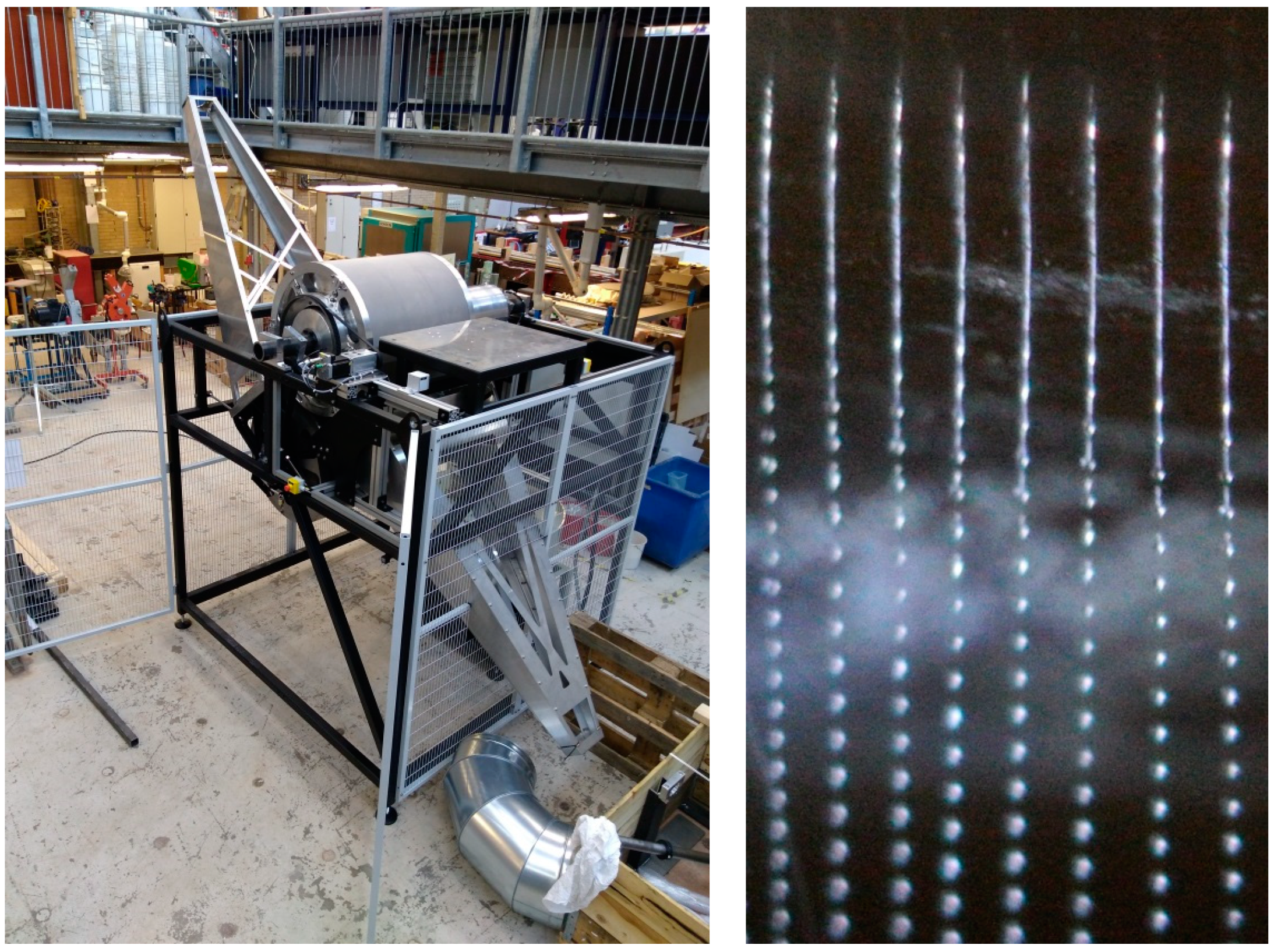
From a mechanical point of view, sensor sorters that are suitable for logarithmic sorting of rigid plastics could, in principle, be built with present technology. Figure 2 shows a prototype with an ejection mechanism based on an array of water jets that is in construction at the Delft laboratory. Logarithmic sorting could be a final step in modern household waste sorting facilities that first recover rigid plastic objects from waste and then purify, wash and flake these streams. Calculations based on data from an advanced packaging waste sorting plant in Amsterdam (PRA) show that a recycling process starting from mixed household waste up to delivery of the recycled plastic to the converter could reach an overall recovery of 70% for rigid plastics, with greenhouse gas emissions of 160 kg of CO2 per ton of recycled plastic (using present Dutch CO2 emissions for electricity and gas). If logarithmic sorting can separate rigid packaging plastics into a large number of homogeneous fractions that could be returned to the original packaging manufacturers and realise full circularity, the increased returns from high-end flake products would also significantly improve the economic feasibility of plastic recycling. The major technology issue is then, whether sensor systems can be developed that can differentiate between all the different materials used for rigid packaging.
Near-infrared spectroscopy (NIRS) is a technology that is commonly used in the separation of main polymer classes, but it has also been shown capable of providing information on characteristics such as the molecular structure [10,20,21] which is inherently related to rheological and mechanical behaviour of plastics [10,11]. Moreover, near-infrared (NIR) spectra have, in combination with mathematical models like principal component analysis (PCA) and partial least squares regression (PLS-R), have already been successfully correlated to for example molecular weight and melt viscosity [22] and to the physiochemical and morphological character [23] of plastics.
In this paper, a new colour plus high resolution NIR-based classification approach for plastic packaging is proposed, that could meet the requirements of circular sorting schemes. This approach was tested in two ways. First, the power of NIR was assessed in distinguishing plastics of the same colour and same main polymer used for different applications, or for the same applications but by different brands. In the second test, material properties that determine the compatibility of plastics in high quality recycling were defined and it was tested whether NIR data measured under ideal conditions on flake pixels could predict those properties. For the tests, plastic objects with a large heterogeneity in non-visual properties were selected.
2. Materials and Methods
2.1. Sample Collection
Within the category of packaging objects, two of the three most used materials are PET and PP. PE, the most used material for packaging, was not included for this study as previous research [22], Ref. [24] already demonstrated the feasibility of predicting the molecular weight and the melt flow rate (MFR) from NIR spectra.
Packaging objects were obtained by purchasing products with a specific packaging rather than by collecting packaging objects from waste, as purchasing allowed easy acquisition of more than one of each object for alternative and repeat analyses. A common colour was selected, natural transparent for both PP and PET, since the objective of the study focused on predicting plastic properties from non-visual characteristics. For each polymer class, three packaging categories were chosen with significant expected differences in strength and rheological requirements. Then, for each of the three packaging categories, different brands were gathered from Dutch stores. For each combination of packaging category and brand, referred to as a packaging class, five pieces were purchased simultaneously at the same store. The 20 packaging classes are listed in Table 1. The polymer class was verified for each object using conventional Fourier-transform infrared spectroscopy (FTIR).
2.2. Compatibility Requirements
The compatibility requirements for plastic waste objects were subdivided into three categories:
- Mechanical compatibility.
- Rheological compatibility.
- Optical compatibility.
In this first step towards a new method for classifying plastics in waste separation, one property for each category was selected. It is noted that the selected properties are not necessarily the most important ones for all mechanical recyclers, but we believe that the selected properties are among the most crucial ones for the average mechanical recycler.
Another note is made with respect to the completeness of these compatibility requirements; the incorporation in or adherence to plastic waste objects of certain functional additives or forbidden and/or hazardous contaminants [25] are also important to consider for the recyclability of waste. Their presence can form a problem when different contaminations chemically react with or due to each other during production processes, having a negative effect on some or several of the aforementioned compatibility requirements [26,27]. Moreover, contaminants, such as some brominated flame retardants, may prohibit the incorporation of the recycled materials in particular products, such as packaging for food applications. The feasibility of differentiating plastics with NIRS based on such additives or contaminants was not investigated in the present study.
2.2.1. Mechanical Compatibility
Mechanical compatibility is relevant for the use phase of a product’s life. More than 10 properties could be considered for compatibility, like tensile strength and creep resistance. Depending on the function and expected lifetime of the product, some properties are more important than others. Based on research conducted by Veelaert et al. [28], tensile strength was selected as one of the most important characteristics to product designers.
Contrary to commonly used testing methods in which tensile specimens are moulded, it was decided to cut specimens for tensile strength measurement directly from the packaging objects. This choice was made as reprocessing the packaging objects would cause thermo-mechanical degradation [11,29], which could influence the mechanical properties of the objects non-uniformly.
A constraint was the limited size of the packaging objects, as a result of which a smaller design for the test specimens had to be made which was not in accordance with ASTM 638 [30]. To ensure unhindered transfer of forces through the specimens, the ratios and angles of specimens as defined in ASTM 638 were followed. Moreover, the same scale was used for all packaging classes. One tensile specimen was cut from each of the five packaging pieces purchased for each packaging class and subsequently cleaned. The tensile tests were thus performed five times for each packaging class, in conformity with conditions specified in ISO 527 [31].
2.2.2. Rheological Compatibility
Rheological compatibility is important during production. More chemically alike plastics are more compatible with each other. This holds both for blends of plastics with the same polymer class [13] and for blends of different polymers [32]. For example, large differences in molecular weight (strongly related to the melt viscosity) within a blend can have a negative impact on the resulting material properties, due to differences in crystallisation [11].
In industry, the processing method, for example injection moulding or blow moulding, dictates the melt viscosity or melt flow index (MFI). Having a known and constant MFI is valuable for processors, as it will optimise production efficiency. It is therefore important that virgin and recycled plastics have the same MFI [33]. Additionally, it is known that upon mixing plastics with different melt viscosities, the material properties will not be uniform after compounding [34].
In this study the melt viscosity was selected to define rheological compatibility. Whereas the melt viscosity is primarily dependent on shear strain and temperature, it was decided to keep the temperature fixed during the measurements. The temperature for each polymer class was set in conformity with the temperature used for conventional MFI measurements, being 280 °C and 230 °C for PET and PP respectively [35,36].
Measurements were performed with an AR G2 (TA Instruments, DE, USA) using parallel plates, under a nitrogen atmosphere to prevent degradative reactions of the polymeric chains with atmospheric oxygen. For each packaging class, one cleaned sample was taken from one of the purchased packaging pieces, with which a strain sweep at constant frequency was conducted first, to determine the shear strain within the linear viscoelastic envelope (LVE). Following the strain sweep, a frequency sweep was performed, using the same sample as used in the strain sweep, with constant strain (within the LVE), varying the frequency between 0.1 and 100 rad/s.
2.2.3. Optical Compatibility
The aesthetic properties of plastic products are important for brands, who use them to differentiate their products. Therefore, technologies exist that can sort plastic waste according to colour. Unfortunately, this is not fully effective, as some plastics will change colour upon being heated to- and/or processed in the melt phase.
For PP, discoloration is thought to be most commonly caused by over-oxidation of phenolic antioxidants (PAO), which give the polymer a yellowish and/or pinkish colour [26,27,37]. Although antioxidants exist that do not cause such discoloration when being (re)processed, for example hindered amine light stabilizers (HALS) [26,37], PAO is still a widely used antioxidant.
To test optical compatibility, one cleaned sample of each of the PP packaging classes was kept in an unventilated atmosphere with high concentrations of NOx for 48 h (gas-fading), a process known to be effective at over-oxidising PAOs [37,38].
For PET, grey discoloration may be caused by reduction of antimony (worldwide the most used catalyst for PET production). Yellowing can be caused by the presence of (polyamide) barriers which are used to reduce permeability [39] and/or by compounds such as quinones and stilbenes which are formed as a result of thermo-oxidation of PET [40]. In conformity with common industrial practices, cleaned PET samples were heated in a ventilated oven under normal atmosphere for 40 min at 220 °C, which would reveal the presence of discolouring compounds such as polyamide barriers, quinones or stilbenes. One sample of each PET packaging class was tested. The occurrence of discoloration for all PP and PET samples was determined visually without instrumentation.
2.3. Spectroscopic Acquisition
For the acquisition of spectral reflectance data, a spectrometer with an effective wavelength range of 895–2523 nm, distributed over 512 spectral pixels, was used. The spectrometer type is NIRQuest-512-2.5 (Ocean Optics, FL, USA) which contains an indium gallium arsenide (InGaAs) detector, type G9208-512W (Hamamatsu Photonics, Japan). The reflected (and emitted) photons were transmitted to the spectrometer through a lab grade optical fibre provided by Ocean Optics, which has a field of view (FOV) of 25.4°. For illumination, a halogen lamp with a bulb colour temperature of 2960 K and a drift of less than 0.1% per hour was used.
Prior to the spectral acquisition, all packaging objects (five per packaging class) were shredded into flakes and cleaned to ensure no foreign materials remained on the surface. The plastic flakes were spread in a monolayer over a carbon black filled polyvinylchloride (PVC) conveyor belt with negligible reflection in the recorded bandwidth, which moved the flakes through the spectrometer vision with low velocity (0.053 m/s) to minimise movement during integration time (19 ms). Reference measurements were obtained by closing the shutter (black reference) and by scanning a piece of Spectralon (Labsphere, NH, USA), a sintered PTFE (Polytetrafluoroethylene) material with a Lambertian reflectance of at least 95% in the analysed spectral range [41].
2.4. Spectral Analyses
The data acquired with the spectrometer were pre-processed, a precursor to effective spectroscopic analysis, using various proven methodologies to separate noise from the signal and to find and enhance relevant spectral features [42,43,44]. Finally, the pre-processed data were analysed using principal component analysis (PCA) and correlated with the measured mechanical and rheological parameters by partial least squares regression (PLS-R).
2.4.1. Pre-Processing
Spectrometers are well known for having bad signal-to-noise-ratio (SNR) at the spectra extremes [42,45]. Additionally, the illumination systems available on the market are not able to provide light with an intensity uniform over the infrared region. Moreover, with spectrometers it can be expected that some defective spectral pixels are present, implying that such pixels have more instrumental noise or are even dead. Both the selection of the usable bandwidth as well as the identification of spikes was done based on the standard deviation (σ) of the signal of the Spectralon under static conditions. The spectral region was limited to 1029–2268 nm for some of the spectroscopic analyses, and within that region 19 pixels were identified as partially defective. For these 19 pixels a median filter (MF) [46] was applied to mitigate the influence that the defect pixels could have on later multivariate analyses.
Outliers can have a detrimental impact on multivariate data analysis by distorting the statistics [47]. Outliers were therefore removed, by taking the mean over all spectra of each packaging class, and subsequently removing of the spectra with the highest mean squared error (MSE) compared to those means.
Differences in light reflection caused by multiplicative effects such as a varying angle of incidence caused by flake orientations, or flake dimensions, are commonly corrected for using multiplicative scatter correction (MSC) [48] or a standard normal variate (SNV) transform [49], of which the latter has been shown to be directly linked to the former [50]. For MSC, two variations were applied, relating to the reference spectrum that is used to regress the spectra to. The first variation used the mean spectrum that was taken over all spectra of one packaging class (piecewise), and the second used the mean spectrum based on all spectra of one polymer class (global). SNV was not used as it had been shown directly linked to MSC and was therefore expected to yield the same results.
Differences in the baseline of spectra, both in terms of baseline shifts as well as for the trend of the baseline, were corrected by normalising the data with the 2nd order polynomial fitted on the mean spectra (piecewise) [49].
Working with derivatives of the spectral data, both 1st and 2nd order, removes any baseline offsets and slopes, comparable to de-trending. Derivations are especially useful for compensating for changes in environmental conditions, such as light intensity, temperature and sample orientation [51,52]. These derivations are also thought to be helpful in distinguishing overlapped spectral peaks [53], something of importance for determining the presence or concentration of specific chemical compounds. The widely accepted method of derivation proposed by Savitzky and Golay [54] was used, hereinafter referred to as Savgol. It is based on a polynomial filter in which the window size and polynomial order are variables that should be considered carefully to avoid amplification of noise while ensuring no important spectral features are removed. Moreover, the Savgol approach has the side effect of smoothing the data. Savgol was also employed without taking derivates, in which case it merely works as a polynomial filter with the sole effect of smoothing. Savitzky and Golay filtering was implemented using SciPy [55].
Another, in many cases effective way of dealing with (instrumental) noise in spectroscopy, is the application of a discrete wavelet transformation (DWT). DWT can be seen as a process of filtering and size reduction [56] in which a filter basis, often referred to as wavelet base, is applied in a linear transformation. Besides filtering noise from the signal of interest, wavelet transformations have also been shown capable of separating spectral features in multispectral images [57], which can be beneficial to classification models like PLS [58]. DWT of a multispectral signal consists of two or more arrays in which one comprises the approximation of the signal and where the rest is formed by wavelet coefficients, the noise. The approximation is the inner product of the original signal and a, discrete and scaled, scaling basis, whereas the wavelet coefficients are the inner product of the signal and a, discrete and scaled, wavelet basis. An infinite number of wavelet and scaling bases can be defined, which makes wavelet transforms broadly applicable. A number of ways for choosing suitable bases is described in literature, such as matching the shape of base functions to the shape of the spectral features of interest [56,58] or more quantitative approaches which try all available bases and measure either the de-noising effect [59] or the performance of a prediction algorithm using leave-one-out cross validation [56]. In this study, the wavelet bases delivering the best prediction performance were chosen. The Python toolbox Pywavelets was used for the wavelet transformations [60].
2.4.2. PCA
Principal component analysis (PCA) is a method used extensively in chemometrics [61], primarily for exploratory data analysis or for the development of predictive models. It simplifies data interpretation by representing multidimensional data in a lower-dimensional space in which the important variations appear. This way, it tries to cluster samples according to physiochemical characteristics [23]. PCA breaks up a spectrum into a number of statistically linearly uncorrelated and orthogonal components, while maximising the variance in leading (principal) components (PCs). Together, the PCs span a new coordinate system in which the recorded spectra are plotted. The most relevant PC’s are used to visualise the distance between clusters of spectra stemming from different packaging classes. Overlapping clusters imply that it may not be feasible to distinguish between packaging classes based on the recorded signal, whereas well segmented populations are separable.
As a first step, the spectra within each packaging class were averaged, so as to minimise the influence of factors not directly related to the plastic objects themselves, such as differences in path length or angle of incidence of illumination. These mean spectra were used to compute the first set of PCs. These PCs thus contained the essential information describing the differences between the packaging classes. Then the original spectra (without having been averaged) were transformed to the coordinate system defined by the PCs, after which each of the packaging classes was represented by an ellipsoidal point cloud. This showed to what extent it is feasible to distinguish between the spectral clouds of the packaging classes, under the influence of random external variables like particle size, recorded location on particle (e.g., edge or centre), particle orientation, surface roughness, path length and intensity of reflected light, taking into account that the variance within each spectral cloud was only attributable to these external variables.
The degree to which packaging classes were differentiable by NIR spectra was determined by defining ellipsoid equations using the variances associated with the set of eigenvectors of each of the point clouds and subsequently counting the number of spectra from other packaging classes that fell within that ellipsoid. A two-dimensional confusion matrix was constructed for each polymer class, indicating the fraction of spectra of packaging class that fell within the ellipsoid covering 95.45% ( from the mean) of the spectra of packaging class . PCA was implemented with in-house software running on Python, using the covariance method based on mean-subtracted data, where the eigenvectors and eigenvalues were distilled from the covariance matrix using Numpy [62].
2.4.3. PLS-R
Partial least squares regression is a widely adopted technique for the development of predictive models, for example with (NIR) spectroscopy where it is primarily used for approximation of concentrations of specific compounds in specimens [44,63], but sometimes also applied for the prediction of other variables which are indirectly or not at all linked to the chemical composition of the analytes [58,64]. PLS-R is related to conventional PCA. What makes PLS-R different, is that it decomposes the signal () into components, latent variables (LVs), while considering the parameters that the regression is made for (material characteristics in this case, -values). LVs are made as to maximise the variance among LVs while also maximising the amount of covariance between and , described by those LVs. The number of LVs used, the pseudo-rank, is important to consider, as too few LVs can result in underfitting, with poor prediction as a result, whereas too many LVs may result in overfitting, implying too much noise is included in the calibration, as a result of which the model will only perform well on the calibration data [47,65] but not on new data.
The performance of the PLS-R model was evaluated for a number of LVs between 1 and (where is equal to the amount of packaging classes of a plastic type), meaning the model was calibrated and validated for every number of LVs. For each number of LVs, the model was calibrated and validated times, each time using a different combination of packaging classes for calibration and 1 class for validation; leave-one-out cross validation. The performance of the model, commonly referred to as the goodness of fit, was evaluated using the root mean squared error of validation (RMSEV) and the coefficient of determination (). The Python toolbox Scikit-Learn was used for implementation of PLS-R [66], which employs the NIPALS algorithm [67].
3. Results
3.1. Material Characteristics
The measured melt viscosity and tensile strength and the observed discoloration are shown in Table 2 for each of the plastic packaging classes. Objects from PP 3.1 were too brittle for cutting tensile test specimens. Since the macromolecules in the plastic objects from which the specimens were cut are not oriented in the same way for each packaging class, as a result of differences in the direction of flow during extrusion, it is expected that anisotropic effects influenced the measured tensile strengths to some extent. For PET packaging categories 1 and 2, all tensile specimens were loaded in the direction of flow during extrusion, whereas the macromolecules in specimens from packaging category 3 had an isotropic orientation. Specimens of PP packaging categories 1 and 3 were loaded at angles of 22.5° and 0° with respect to the direction of flow during extrusion, respectively. Macromolecules in the specimens cut from PP packaging category 2 had a varying orientation as the point of injection during extrusion was in the centre of the surface of those specimens.
During the measurements of the melt viscosity for PET, it was observed that the material degraded, which became apparent as the viscosity increased under constant conditions with the passing of time. This is a known behaviour of PET when heated to temperatures already as high as 200 °C, even in a nitrogen atmosphere [68]. It was decided to use the melt viscosity measured shortly after the start of the measurement cycle, namely the viscosity at 1 Hz (1.5 min after the start of the frequency sweep and 5 min after the start of the strain sweep) in order to minimise the effect that degradation could have on the results of multivariate analyses. As it is known that the melt viscosity increased by 14% during one frequency sweep of 12 min, it could be assumed that the effect of degradation on the measured viscosity at 1 Hz was less than 14%.
All but one packaging class for PP showed significant discoloration. Therefore, optical compatibility of PP packaging classes was left out from statistical analysis, as the unbalanced dataset would not allow the production of a meaningful classification model. It is noted however, that it has been proven in other research that PAO can be detected, and to a certain extent quantified, in PE using NIRS [63]. It is therefore thought likely that this is also feasible for PAO in PP. With regards to the optical compatibility of PET, the observed number of different modes of discoloration (five), was too large compared to the size of the dataset, for the development of a model. Therefore, it was decided to omit this property from statistical analyses as well.
3.2. Analysis
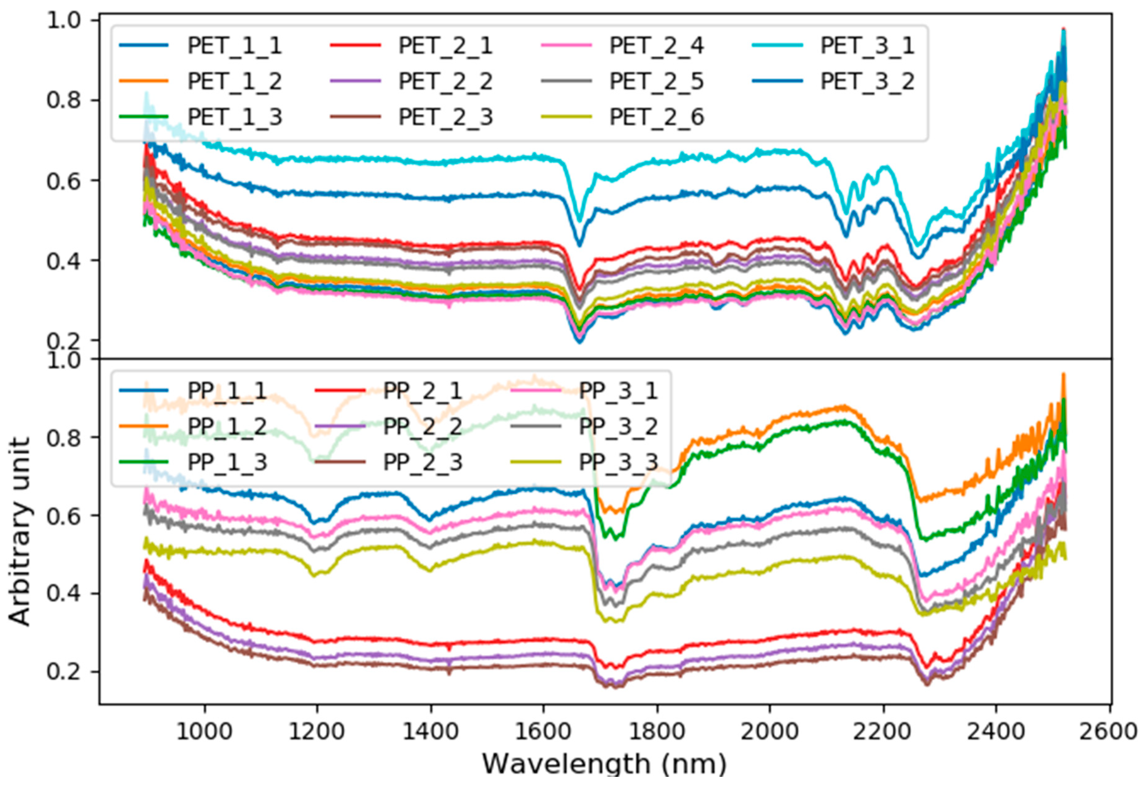
The recorded spectra of each plastic packaging class were filtered to remove pixels which just captured the conveyor belt. After filtering, between 69 and 777 recorded spectra remained for each of the 20 analysed packaging classes. The average number of recorded spectra per flake was not recorded. It is therefore possible that the (averaged) spectra of some packaging classes can be based on a more varied dataset, in terms of flake size and orientation, than others. The normalised and averaged spectra (prior to pre-processing) are plotted in Figure 3.
Results of PCA and PLS-R were evaluated to get an indication of the feasibility of differentiating between packaging objects of the same plastic type and of predicting the melt viscosity and tensile strength of plastic packaging objects using NIRS.
3.2.1. PCA
PCA was applied on the packaging class-averaged spectral data for PET/PP, after some basic spectral pre-processing (normalisation, spike mitigation, scatter correction and smoothing) of the pixel data. After transformation of the pre-processed pixel-data to the PCA-space and subsequently defining ellipse equations for each of the packaging classes’ point clouds, the extent of overlap of the packaging classes could be assessed. The resulting confusion matrices for PET and PP, provided in Table 3 and Table 4, indicate that the tested PET and PP packaging classes are, with few exceptions, well distinguishable using NIRS of single pixels.
The total confusion, here defined as the sum of all off-diagonal percentages, for PET and PP was 6% and 47% respectively, whereas complete confusion would give 11000% and 7200% respectively. Upon looking closer at the three pairs of classes that were not completely distinguishable (PET 3.1/3.2, PP 2.1/2.2 and PP 3.1/3.2), it is noted that for PET 3.1/3.2 and PP 3.1/3.2 no major differences in tensile strength and viscosity were measured: from 1% to 5% of the maximum measured values. For PP 2.1/2.2 the differences in material characteristics were however significant: 11% of the maximum measured values.
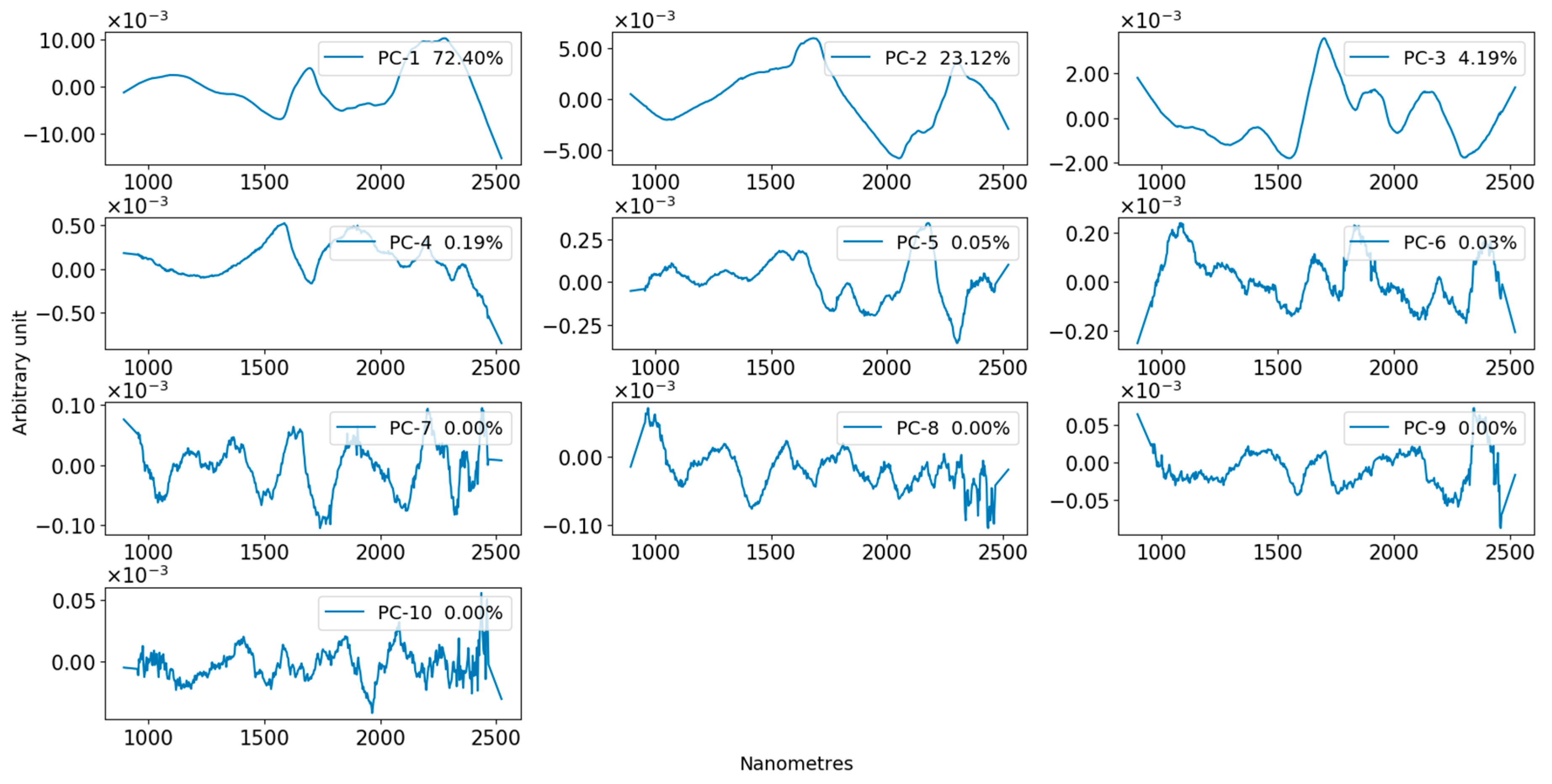
Loadings of the PCs based on the averaged spectra were analysed. Loadings were created by multiplying the PCs with the square root of eigenvalues. Figure 4 and Figure 5 show all PC loadings for the PCs that span the coordinate systems used to create the confusion matrices of Table 3 and Table 4. The legends in these figures also mention the percentage of the variance of the averaged spectra that is explained by each principal component.
The importance of individual PCs in the differentiation of the packaging classes was determined by selectively leaving out dimensions (PCs) and determining the resulting increase in total confusion.
It was found that for PET, the 3rd, 6th and 9th PCs were of least importance for differentiation of the packaging classes, with an increase of total confusion of 462%, 207% and 680% respectively. Excluding any of the other PCs increased the total confusion by a minimum of 1957%. Next, it was investigated whether certain PCs contributed specifically to the differentiation of particular packaging classes or packaging categories. Some patterns were observed, for instance that the exclusion of certain PCs rendered the distinction between two or more particular classes infeasible, while not, or barely, affecting the distinction between other classes. Upon excluding the 5th PC for example, the point cloud containing 95.45% of the points of PET 3.2, held on average 87.5% of the points of all other objects, thus making its differentiation impossible. Meanwhile the differentiation of other packaging classes was influenced significantly less. This suggests that the information captured in some of the PCs describes specific compounds or other material-related factors that are characteristic for some of the packaging classes/categories. It can be expected for instance, that some PCs describe the compounds glycol and antimony (the most used catalyst for the production of PET), since these are expected to be present in varying concentrations in the PET objects. Within this study loadings were not correlated to specific compounds.
For the PP packaging classes, it was found that the only PC of which exclusion did not lead to an increase in total confusion of more than 1000%, was the 8th PC (550%). It is noted that the effect of exclusion of various PCs on the total confusion showed a very clear packaging category related dependency, in which the differentiation within particular packaging categories deteriorated while the ability to distinguish between other packaging categories changed much less. An example is the exclusion of the 8th PC, which made the differentiation within Categories 2 and 3 impossible for most pairs, while the differentiation of all other classes was virtually unaffected. Moreover, upon the exclusion of the 6th PC, classes within all categories were no longer well differentiable, while simultaneously packaging Categories 1 and 3 were no longer differentiable. The differentiation of classes in Category 2 from classes in Categories 1 and 3 was however almost entirely unaffected. This last example is illustrated with the resulting confusion matrix, as depicted in Table 5, in which a colour scale is implemented for better overview.
These examples illustrate for PP that the materials’ chemical contents and/or (molecular) structures stemming from the different packaging categories were truly different between those categories while being more similar within the categories. In this context, it can be expected that one or more of the PCs were directly or indirectly related to the tactility of the macromolecules and perhaps also the molecular weight, properties that vary between resins, and are influenced, among other things, by the use of catalysts, such as Ziegler–Natta and metallocene catalysts [69]. As it can be expected that those catalysts have an effect on the recorded spectra, they may form (possibly among other things) the differentiating factor for classes within the same packaging categories.
The effect of the exclusion of the 6th PC shows that PP packaging classes from Categories 1 and 3 have something dissimilar which is captured within that PC. Perhaps a certain additive (type) was used in the objects of one of these packaging categories, particular to the intended use of packaging objects within that category.
3.2.2. Correlating Principal Components to Viscosity and Tensile Strength
To see with which areas of the NIR spectrum the measured material characteristics were most correlated, the projections of the averaged pre-processed spectra of each packaging class on the principal components were stored in rows of the matrix while the measured material characteristics for each packaging class were stored in the vector . The vector was calculated to satisfy Equation (1) in the least square sense. The natural logarithm of the melt viscosity was used as a parameter for the rheology, in line with previous research on the development of regression models for the prediction of rheological parameters [70].
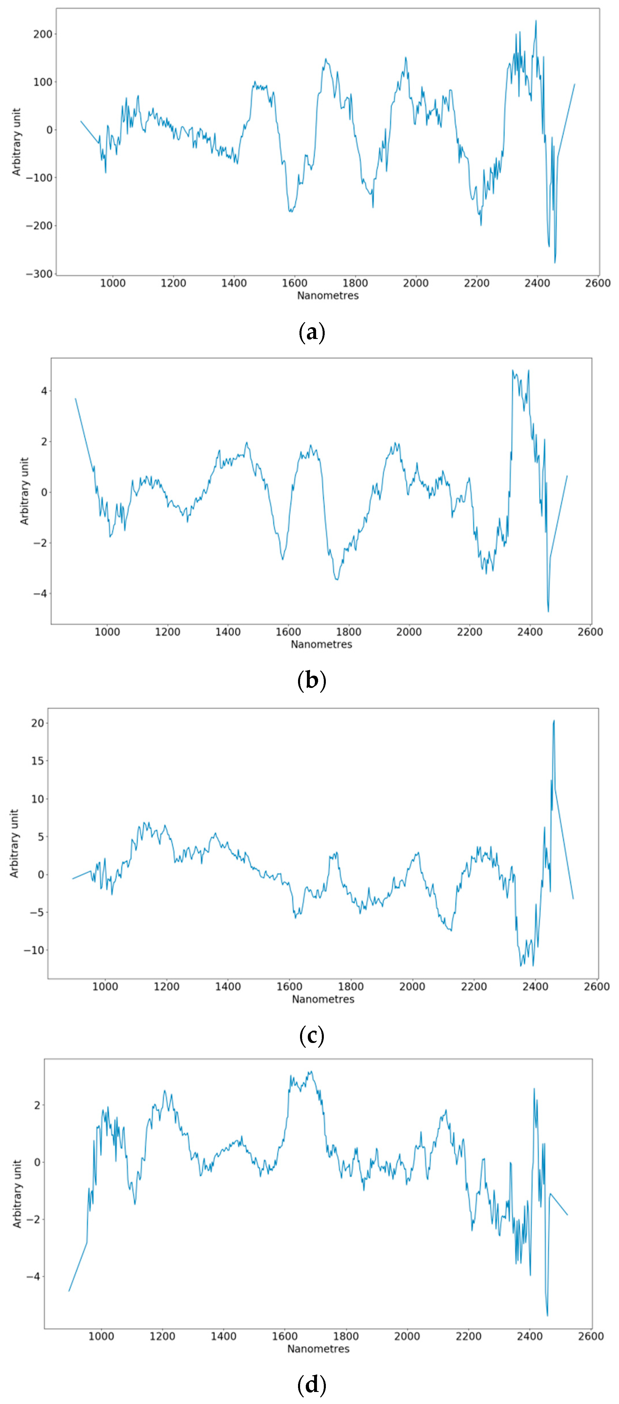
For the two plastic types and the two measured material characteristics, this overdetermined system with unknowns (one coefficient per PC) and equations, where equals the number of classes, was solved using a least squares approach. The resulting coefficients, shown in Table 6 and Table 7 for PET and PP, respectively, indicate the correlation of the PCs with the material characteristics. Figure 6 gives the theoretical spectra of the material characteristics, obtained by multiplying the coefficients with the corresponding PC loadings of Figure 4 and Figure 5. Finally, Table 8 shows the coefficients of determination and the root mean squared error of calibration (RMSEC) for the best fits.
3.2.3. PLS
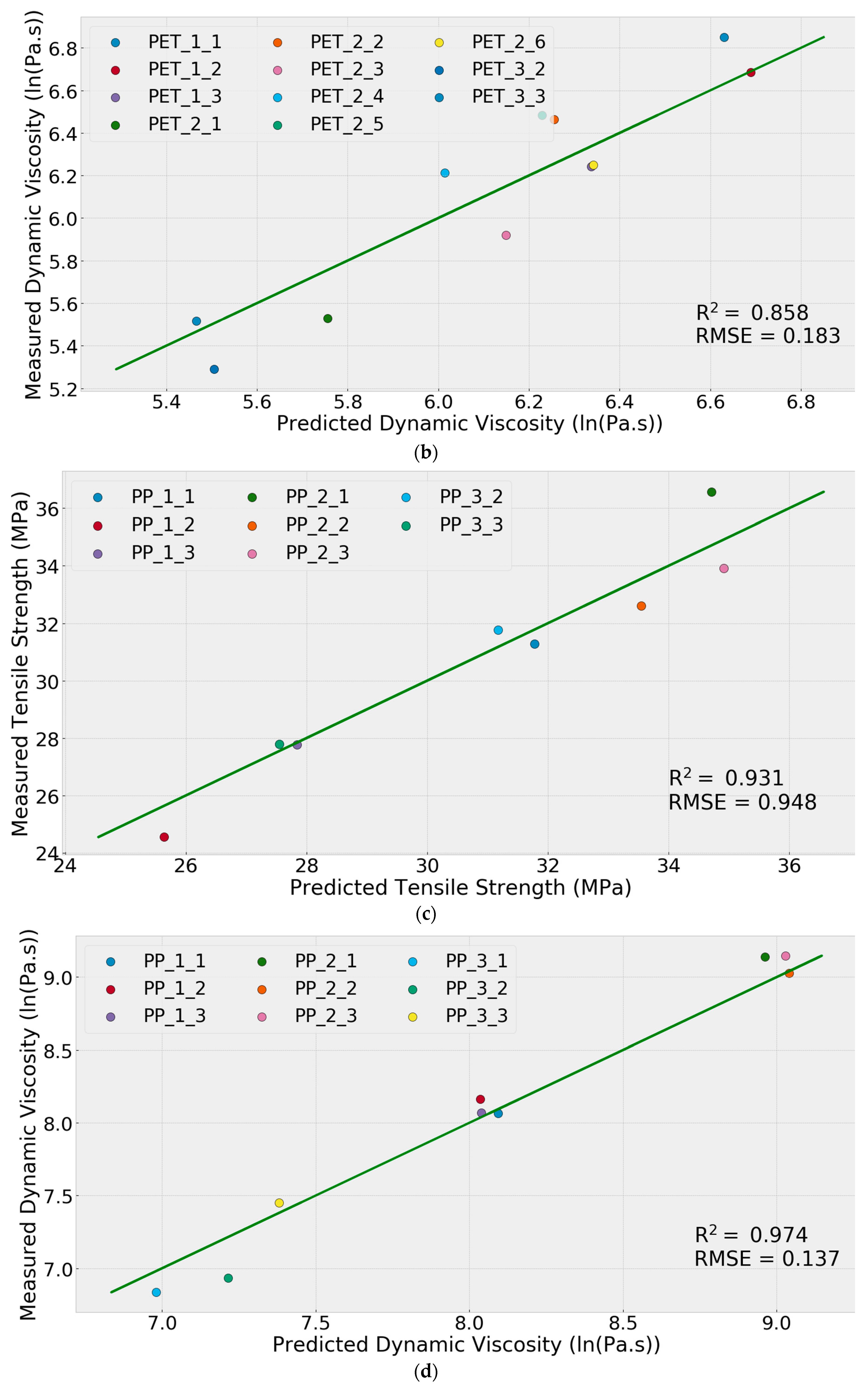
PLS-R models for the prediction of the tensile strength and melt viscosity of PET and PP packaging objects were calibrated and validated. For the melt viscosity, the natural logarithms of the measured quantities were used. The performance parameters of the models, including the used pre-processing techniques, are presented in Table 9. Graphs with the measured and predicted parameters are provided in Figure 7, in which the green trend line represents perfect prediction. The prediction performance is best assessed by relating the prediction errors to the spread of the measured Y values, which show that the root mean squared error of validation (RMSEV) varied between 5.67% (PP melt viscosity) and 17.80% (PET tensile strength) of the total spread.
4. Discussion
PCA shows that it is practically feasible to differentiate the tested plastic packaging objects based on single-pixel NIRS. For example, the confusion between food and non-food PET packaging, a distinction of major importance for recycling, was well below the 5% limit observed by recyclers. PP packaging objects with the same function (e.g., lid of dairy container) but of different brands, were more difficult to distinguish than packaging objects with different functions, as the omission of certain principal components from the analysis rendered the differentiation within packaging categories infeasible while barely affecting the differentiation between packaging categories. This links with the observation that the considered material characteristics for PP objects were more similar within the packaging categories while being more dissimilar between the categories. This finding suggests that separating plastic packaging objects on their function may be feasible and beneficial for the quality of the resulting recycled plastics. In this context it is noted that the presence of specific groups of functional additives, for example UV-stabilisers, was also correlated with the function of the packaging objects, which makes it even more desirable to separate packaging objects based on their functions, as dosing of additives during reprocessing could then be decreased. For PET, no clear correlation between the measured material characteristics and the function of the packaging objects was found, apart from Category 3 (blister packs). Meanwhile, for PET no PCs were found whose exclusion showed a clear packaging category dependent effect on the differentiation.
The conditions of the tests are to some extent comparable to industry, since parameters with values that are typical for industry, such as the sizes of the plastic flakes, their orientation on the conveyor belt, the section of the flakes that was recorded (e.g., edge or centre), pixel size, surface roughness, angle of incidence and the path length, with few exceptions did not hinder the differentiation. Industrial conditions which could hinder the differentiation are the presence of moisture, severely degraded materials and residual non-plastic contaminations (e.g., proteins and grease) and a more limited data bandwidth of NIR spectra.
Further analysis of the principal components and latent variables and/or enlargement of the variance (objects from waste streams, different geographical origins and different degrees of degradation and residual contamination) in the dataset is required to confirm that plastic packaging objects that are incompatible for high-end recycling are generally differentiable, and also that the tensile strength and melt viscosity of packaging objects are predictable from single pixel NIR data. Circumstances such as the time a product spent on the shelf in the store before it was bought (relating to UV degradation) or the temperature at which the material was processed during extrusion (relating to degradation by oxidation) could possibly affect the spectra as well.
5. Conclusions
A study was carried out to assess the feasibility of a circular route for rigid plastic packaging based on an innovative low-cost and low-CO2 mechanical sorting process that would allow recyclers to return flakes from EOL packaging to the original manufacturers of the packaging. It was shown that a critical condition for implementing the process is the existence of an affordable sensor system that can differentiate between a large number of packaging plastic grades. Preferably this differentiation is based on properties of the plastic that are important for applications, production processes and brands. This study investigated a combination of colour and high-resolution NIR as a potential candidate for the sensor system. Taking for granted that such a system can recognize the colour and main polymer class of a flake on the basis of a single pixel response, a hierarchy of transparent PET packaging objects and a hierarchy of transparent PP packaging objects were tested to see if NIRS can distinguish between applications and brands. At the top level of the hierarchy, packaging objects differed in application (e.g., soap vs. beverage vs. hardware) while at the bottom level objects with the same application differed only by brand. The conceptual basis of the test setup was that different applications may require different additives or rheological and mechanical properties of the plastic, while different brands may choose different additives for the same functionality. In total, 100 objects of 11 polyethylene terephthalate (PET) and nine polypropylene (PP) packaging classes of different brands and functions were purchased in Dutch stores and their melt viscosity, tensile strength and potential discoloration during reprocessing were determined using samples cut from the objects. Afterwards, the objects were flaked and cleaned and a multitude of NIR spectra were obtained of single pixels of flakes under perfect conditions, after careful washing and drying of the flakes, and using a wide spectral range of 895–2523 nm.
Principal component analysis (PCA) demonstrated the feasibility of distinguishing between plastic packaging objects of the same colour and plastic type with single-pixel NIR data. It was shown that the clusters of NIR spectra from the various packaging classes had almost no overlap in the reduced dimensional PC space, implying that variables such as particle size, orientation, surface roughness, angle of incidence and path length, variables that cannot be controlled in an industrial setting, did not significantly hinder differentiation.
The gathered datasets were too small and/or too diverse to be able to create models for characterisation of the plastic packaging classes in terms of discolouration. However, models with sufficient accuracy for flake sorting for the prediction of the melt viscosity and tensile strength of the purchased packaging classes were developed using NIRS data. The calibrated regression models for the prediction of the viscosities of PET (11 objects in dataset, spread of 1.56 ln(Pa.s)) and PP (nine objects in dataset, spread of 2.31 ln(Pa.s)) had a root mean squared error of validation (RMSEV) of 0.183 and 0.137 ln(Pa.s) respectively, with coefficients of determination () of 0.858 and 0.974 respectively. Moreover, regression models predicted the tensile strengths of PET (11 objects in dataset, spread of 59.28 MPa) and PP (eight objects in dataset, spread of 12.02 MPa) with RMSEVs of 10.55 and 0.95 MPa respectively, with of 0.711 and 0.931 respectively. These results are comparable with results by Hansen et al. [70] and by Saeki et al. [22] who demonstrated the successful prediction of melt flow index (MFI) in polyethylene vinyl acetate (EVA), with a RMSEV of 0.46 ln(MI) on a spread of 5.55 ln(MI), and polyethylene (PE), with a RMSEV of 0.038 g/10 min on a spread of 99.96 g/10 min, respectively.
It is concluded that colour plus high-resolution NIR is a promising sensor system for recycling rigid packaging plastics into high-grade products. A particular advantage of sorting on NIR over sorting on brand-specific markers is that NIR yields direct information on additives and rheological properties. This reduces the risk that polymer recipes used by the same brand and packaging change in time, with the result that incompatible additives get mixed in recycling. This advantage may also expand the number of outlets for a recycler because plastics of different packaging brands that happen to be functionally indistinguishable need not be sorted into different products.
Author Contributions
Conceptualization, Y.v.E. and P.R.; methodology, Y.v.E., M.B., R.B. and P.R.; software, Y.v.E.; validation, Y.v.E.; investigation, Y.v.E., P.W.; data curation, Y.v.E.; writing—original draft preparation, Y.v.E. and P.R.; writing—review and editing, Y.v.E., P.W., M.B., R.B. and P.R.
Funding
This research received no external funding.
Conflicts of Interest
The authors declare no conflict of interest.
References and Notes
- PlasticsEurope. Plastics—The Facts 2017; PlasticsEurope: Belgium, Brussels, 2018. [Google Scholar]
- Van Eygen, E.; Laner, D.; Fellner, J. Circular economy of plastic packaging: Current practice and perspectives in Austria. Waste Manag. 2018, 72, 55–64. [Google Scholar] [CrossRef] [PubMed]
- Brouwer, M.T.; Van Velzen, E.U.T.; Augustinus, A.; Soethoudt, H.; De Meester, S.; Ragaert, K. Predictive model for the Dutch post-consumer plastic packaging recycling system and implications for the circular economy. Waste Manag. 2018, 71, 62–85. [Google Scholar] [CrossRef] [PubMed] [Green Version]
- de Souza Machado, A.A.; Kloas, W.; Zarfl, C.; Hempel, S.; Rillig, M.C. Microplastics as an Emerging Threat to Terrestrial Ecosystems. Glob. Chang. Biol. 2018, 24, 1405–1416. [Google Scholar] [CrossRef] [PubMed]
- Carrasco, P.A.; Harvey, M.B.; Saravia, A.M. The rare Andean pitviper Rhinocerophis jonathani (Serpentes: Viperidae: Crotalinae): Redescription with comments on its systematics and biogeography. Zootaxa 2009, 2283, 1–15. [Google Scholar] [CrossRef]
- Derraik, J.G.B. The pollution of the marine environment by plastic debris: A review. Mar. Pollut. Bull. 2002, 44, 842–852. [Google Scholar] [CrossRef]
- Di Maio, F.; Rem, P.C.; Baldé, K.; Polder, M. Resources, Conservation and Recycling Measuring resource efficiency and circular economy: A market value approach. Resour. Conserv. Recycl. 2017, 122, 163–171. [Google Scholar] [CrossRef]
- Finnveden, G.; Johansson, J.; Lind, P.; Moberg, Å. Life cycle assessment of energy from solid waste—part 1: General methodology and results. J. Clean. Prod. 2005, 13, 213–229. [Google Scholar] [CrossRef]
- Maris, J.; Bourdon, S.; Brossard, J.-M.; Cauret, L.; Fontaine, L.; Montembault, V. Mechanical recycling: Compatibilization of mixed thermoplastic wastes. Polym. Degrad. Stab. 2018, 147, 245–266. [Google Scholar] [CrossRef]
- Vilaplana, F.; Karlsson, S. Quality Concepts for the Improved Use of Recycled Polymeric Materials: A Review. Macromol. Mater. Eng. 2008, 293, 274–297. [Google Scholar] [CrossRef]
- La Mantia, F.P. Basic Concepts on the Recycling of Homogeneous and Heterogeneous Plastics. In Recycling of PVC and Mixed PLASTIC Waste; Chem Tec Publishing: Toronto, ON, Canada, 1996; pp. 63–76. [Google Scholar]
- Mendes, A.; Cunha, A.; Bernardo, C.; Mendes, A.; Bernardo, C. Study of the degradation mechanisms of polyethylene during reprocessing. Polym. Degrad. Stab. 2011, 96, 1125–1133. [Google Scholar] [CrossRef]
- Ragaert, K.; Delva, L.; Van Geem, K. Mechanical and chemical recycling of solid plastic waste. Waste Manag. 2017, 69, 24–58. [Google Scholar] [CrossRef] [PubMed]
- Al-Salem, S.; Lettieri, P.; Baeyens, J. The valorization of plastic solid waste (PSW) by primary to quaternary routes: From re-use to energy and chemicals. Prog. Energy Combust. Sci. 2010, 36, 103–129. [Google Scholar] [CrossRef]
- Simon, J.M. Beverage packaging and Zero Waste. 2010. Available online: https://zerowasteeurope.eu/tag/germany-deposit-refund-system/ (accessed on 24 October 2018).
- Luijsterburg, B.; Goossens, H.; Goossens, J. Assessment of plastic packaging waste: Material origin, methods, properties. Resour. Conserv. Recycl. 2014, 85, 88–97. [Google Scholar] [CrossRef]
- Serranti, S.; Luciani, V.; Bonifazi, G.; Hu, B.; Rem, P.C. An innovative recycling process to obtain pure polyethylene and polypropylene from household waste. Waste Manag. 2015, 35, 12–20. [Google Scholar] [CrossRef]
- Flory, P.J. Thermodynamics of High Polymer Solutions. J. Chem. Phys. 1942, 10, 51. [Google Scholar] [CrossRef]
- Dahmus, J.B.; Gutowski, T.G. What Gets Recycled: An Information Theory Based Model for Product Recycling. Environ. Sci. Technol. 2007, 41, 7543–7550. [Google Scholar] [CrossRef]
- Huang, J.; Hong, J.; Urban, M. Attenuated total reflectance Fourier transform infra-red studies of crystalline-amorphous content on polyethylene surfaces. Polymer 1992, 33, 5173–5178. [Google Scholar] [CrossRef]
- Baker, C.; Maddams, W.F. Infrared Spectroscopic Studies on Polyethylene, 1 The Measurement of Low Levels of Chain Branching. Die Makromol. Chem. 1976, 987, 437–448. [Google Scholar] [CrossRef]
- Saeki, K.; Tanabe, K.; Matsumoto, T.; Uesaka, H.; Amano, T.; Funatsu, K. Prediction of Polyethylene Density by Near-Infrared Spectroscopy Combined with Neural Network Analysis. J. Comput. Chem. Jpn. 2003, 2, 33–40. [Google Scholar] [CrossRef] [Green Version]
- Papini, M. Analysis of the reflectance of polymers in the near- and mid-infrared regions. J. Quant. Spectrosc. Radiat. Transf. 1997, 57, 265–274. [Google Scholar] [CrossRef]
- Bonifazi, G.; Capobianco, G.; Serranti, S. A Hierarchical Classification Approach for Recognition of Low-Density (LDPE) and High-Density Polyethylene (HDPE) in Mixed Plastic Waste Based on Short-Wave Infrared (SWIR) Hyperspectral Imaging. Spectrochim. Acta Part A Mol. Biomol. Spectrosc. 2018, 198, 115–122. [Google Scholar] [CrossRef] [PubMed]
- Leslie, H.; Leonards, P.; Brandsma, S.; De Boer, J.; Jonkers, N. Propelling plastics into the circular economy—weeding out the toxics first. Environ. Int. 2016, 94, 230–234. [Google Scholar] [CrossRef] [PubMed]
- Kikuchi, T.; Ohtake, Y.; Tanaka, K. Discoloration Phenomenon Induced by the Combination of Phenolic Antioxidants & Hindered Amine Light Stabilisers. Int. Polym. Sci. Technol. 2013, 40, 7–13. [Google Scholar]
- Pospíšil, J.; Habicher, W.D.; Pilař, J.; Nešpůrek, S.; Kuthan, J.; Piringer, G.O.; Zweifel, H. Discoloration of Polymers by Phenolic Antioxidants. Polym. Degrad. Stab. 2002, 77, 531–538. [Google Scholar] [CrossRef]
- Veelaert, L.; Bois, E.D.; Ragaert, K. Design from Recycling. In Proceedings of the International Conference of the DRS Special Interest Group on Experiential Knowledge at Estonian Academy of Arts, Delft, The Netherlands, 19–20 June 2017. [Google Scholar]
- Strömberg, E.; Karlsson, S. The design of a test protocol to model the degradation of polyolefins during recycling and service life. J. Appl. Polym. Sci. 2009, 112, 1835–1844. [Google Scholar] [CrossRef]
- ASTM International. Standard Test Method for Tensile Properties of Plastics; ASTM International: Montgomery County, PA, USA, 2003. [Google Scholar]
- NEN-EN-ISO 527-1. 2012.
- Koning, C. Strategies for compatibilization of polymer blends. Prog. Polym. Sci. 1998, 23, 707–757. [Google Scholar] [CrossRef]
- Sigbritt, K. Recycled Polyolefins. Material Properties and Means for Quality Determination. In Long Term Properties of Polyolefins; Springer: Berlin/Heidelberg, Germany, 2004; pp. 201–230. [Google Scholar]
- Hu, B.; Serranti, S.; Fraunholcz, N.; Di Maio, F.; Bonifazi, G. Recycling-oriented characterization of polyolefin packaging waste. Waste Manag. 2013, 33, 574–584. [Google Scholar] [CrossRef]
- NEN-ISO 12418-2. 2012.
- NEN. NEN-EN-ISO 1873-2. 2007.
- Gijsman, P. Polymer Stabilization. In Applied Plastics Engineering Handbook; Elsevier: Amsterdam, The Netherlands, 2017; pp. 395–422. [Google Scholar]
- King, R.E. Discoloration Resistant Polyolefin Films. J. Plast. Film Sheeting 2002, 18, 179–211. [Google Scholar] [CrossRef]
- Berg, D.; Schaefer, K.; Koerner, A.; Kaufmann, R.; Tillmann, W.; Moeller, M. Reasons for the Discoloration of Postconsumer Poly(ethylene terephthalate) during Reprocessing. Macromol. Mater. Eng. 2016, 301, 1454–1467. [Google Scholar] [CrossRef]
- Edge, M.; Allen, N.; Wiles, R.; McDonald, W.; Mortlock, S. Identification of luminescent species contributing to the yellowing of poly(ethyleneterephthalate) on degradation. Polymer 1995, 36, 227–234. [Google Scholar] [CrossRef]
- Georgiev, G.T.; Butler, J.J. Long-term calibration monitoring of Spectralon diffusers BRDF in the air-ultraviolet. Appl. Opt. 2007, 46, 7892–7899. [Google Scholar] [CrossRef] [PubMed]
- Esquerre, C.; Gowen, A.; Burger, J.; Downey, G.; O’Donnell, C.; Gowen, A. Suppressing sample morphology effects in near infrared spectral imaging using chemometric data pre-treatments. Chemom. Intell. Lab. Syst. 2012, 117, 129–137. [Google Scholar] [CrossRef]
- Vidal, M.; Amigo, J.M. Chemometrics and Intelligent Laboratory Systems Pre-Processing of Hyperspectral Images. Essential Steps before Image Analysis. Chemom. Intell. Lab. Syst. 2012, 117, 138–148. [Google Scholar] [CrossRef]
- Grahn, F.H.; Geladi, P. Techniques. In Techniques and Applications of Hyperspectral Image Analysis; John Wiley & Sons: Hoboken, NJ, USA, 2007. [Google Scholar]
- Ferrari, C.; Foca, G.; Calvini, R.; Ulrici, A. Fast exploration and classification of large hyperspectral image datasets for early bruise detection on apples. Chemom. Intell. Lab. Syst. 2015, 146, 108–119. [Google Scholar] [CrossRef] [Green Version]
- Feuerstein, D.; Parker, K.H.; Boutelle, M.G. Practical Methods for Noise Removal: Applications to Spikes, Nonstationary Quasi-Periodic Noise, and Baseline Drift. Anal. Chem. 2009, 81, 4987–4994. [Google Scholar] [CrossRef]
- Martens, H.; Næs, T. Multivariate Calibration; John Wiley & Sons Ltd.: New York, NY, USA, 1989. [Google Scholar]
- Geladi, P.; MacDougall, D.; Martens, H. Linearization and Scatter-Correction for Near-Infrared Reflectance Spectra of Meat. Appl. Spectrosc. 1985, 39, 491–500. [Google Scholar] [CrossRef]
- Barnes, R.J.; Dhanoa, M.S.; Lister, S.J. Standard Normal Variate Transformation and De-Trending of Near-Infrared Diffuse Reflectance Spectra. Appl. Spectrosc. 1989, 43, 772–777. [Google Scholar] [CrossRef]
- Dhanoa, S.M.; Lister, S.J.; Sanderson, R.; Barnes, R.J. The Link between Multiplicative Scatter Correction (MSC) and Standard Normal Variate (SNV) Transformations of NIR Spectra. Near Infrared Spectrosc. 1994, 2, 43–47. [Google Scholar] [CrossRef]
- Giesbrecht, F.G.; McClure, W.F.; Hamid, A. The Use of Trigonometric Polynomials to Approximate Visible and near Infrared Spectra of Agricultural Products. Appl. Spectrosc. 1981, 35, 210–214. [Google Scholar] [CrossRef]
- Norris, H.K.; Williams, P.C. Optimization of Mathematical Treatments of Raw Near-Infrared Signal in the Measurement of Protein in Hard Red Spring Wheat. I. Influence of Particle Size. Cereal Chem. 1984, 61, 158–164. [Google Scholar]
- Feng, Y.-Z.; Sun, D.-W. Near-infrared hyperspectral imaging in tandem with partial least squares regression and genetic algorithm for non-destructive determination and visualization of Pseudomonas loads in chicken fillets. Talanta 2013, 109, 74–83. [Google Scholar] [CrossRef] [PubMed]
- Savitzky, A.; Golay, M.J.E. Smoothing and Differentiation of Data by Simplified Least Squares Procedures. Anal. Chem. 1964, 36, 1627–1639. [Google Scholar] [CrossRef]
- Jones, E.; Oliphant, E.; Peterson, P. SciPy: Open Source Scientific Tools for Python. 2001. Available online: https://www.researchgate.net/publication/213877848_SciPy_Open_Source_Scientific_Tools_for_Python (accessed on 08 November 2019).
- Mcnulty, S.C.; Mauze, G. Applications of Wavelet Analysis for Determining Glucose Concentration of Aqueous Solutions Using NIR Spectroscopy Applications of Wavelet Analysis for Determining Glucose Concentration of Aqueous Solutions Using NIR Spectroscopy. In Proceedings of the 98 International Biomedical Optics Symposium, San Jose, CA, USA, 27 January 1998. [Google Scholar]
- Bruce, L.; Koger, C.; Li, J. Dimensionality reduction of hyperspectral data using discrete wavelet transform feature extraction. IEEE Trans. Geosci. Remote. Sens. 2002, 40, 2331–2338. [Google Scholar] [CrossRef]
- Kim, G.; Kim, D.-Y.; Kim, G.H.; Cho, B.-K. Applications of Discrete Wavelet Analysis for Predicting Internal Quality of Cherry Tomatoes using VIS/NIR Spectroscopy. J. Biosyst. Eng. 2013, 38, 48–54. [Google Scholar] [CrossRef] [Green Version]
- Hu, S.; Hu, Y.; Wu, X.; Li, J.; Xi, Z.; Zhao, J. Research of Signal De-noising Technique Based on Wavelet. Telkomnika Indones. J. Electr. Eng. 2013, 11, 5141–5149. [Google Scholar] [CrossRef]
- Lee, G.; Gommers, R.; Wasilewski, F.; Wohlfahrt, K.; O’Leary, A.; Nahrstaedt, H. PyWavelets—Wavelet Transforms in Python. 2006. Available online: https://zenodo.org/record/2634243#.XcUF8WYRWUl (accessed on 12 October 2018).
- Bro, R.; Smilde, A.K. Principal Component Analysis. Anal. Methods 2014, 6, 2812–2831. [Google Scholar] [CrossRef]
- Van Der Walt, S.; Colbert, S.C.; Varoquaux, G. The NumPy Array: A Structure for Efficient Numerical Computation. Comput. Sci. Eng. 2011, 13, 22–30. [Google Scholar] [CrossRef] [Green Version]
- Camacho, W.; Karlsson, S. Quantification of Antioxidants in Polyethylene by Near Infrared ( NIR ) Analysis and Partial Least Squares ( PLS ) Regression. Int. J. Polym. Anal. Charact. 2013, 7, 37–41. [Google Scholar] [CrossRef]
- Pornprasit, R.; Pornprasit, P.; Boonma, P.; Natwichai, J. A Study on Prediction Performance of the Mechanical Properties of Rubber Using Fourier-Transform near Infrared Spectroscopy. J. Near Infrared Spectrosc. 2018, 26, 351–358. [Google Scholar] [CrossRef]
- Martens, H.; Martens, M. Modified Jack-knife estimation of parameter uncertainty in bilinear modelling by partial least squares regression (PLSR). Food Qual. Prefer. 2000, 11, 5–16. [Google Scholar] [CrossRef]
- Pedregosa, F.; Varoquaux, G.; Gramfort, A.; Michel, V.; Thirion, B.; Grisel, O.; Blondel, M.; Prettenhofer, P.; Weiss, R.; Dubourg, V.; et al. Scikit-Learn: Machine Learning in Python. J. Mach. Learn. Res. 2011, 12, 2825–2830. [Google Scholar]
- Wold, H. Research Papers in Statistics; David, F., Ed.; John Wiley and Sons: London, UK, 1966; pp. 411–444. [Google Scholar]
- Dzicio, M.; Trzeszczyski, J.; Dzięcioł, M.; Trzeszczyński, J. Volatile products of poly(ethylene terephthalate) thermal degradation in nitrogen atmosphere. J. Appl. Polym. Sci. 2000, 77, 1894–1901. [Google Scholar] [CrossRef]
- Shamiri, A.; Chakrabarti, M.H.; Jahan, S.; Hussain, M.A.; Kaminsky, W.; Aravind, P.V.; Yehye, W.A. The Influence of Ziegler-Natta and Metallocene Catalysts on Polyolefin Structure, Properties, and Processing Ability. Materials 2014, 7, 5069–5108. [Google Scholar] [CrossRef] [PubMed]
- Hansen, G.M.; Vedula, S. In-Line Fiber-Optic Near-Infrared Spectroscopy: Monitoring of Rheological Properties in an Extrusion Process. Part I. J. Appl. Polym. Sci. 1997, 68, 859–872. [Google Scholar] [CrossRef]
Figure 1.
Graphical scheme of a sorting plant inspired by Shannon. The heaps of plastics represent bunkers for storage of intermediate mixtures while the circular disks are programmable binary sensor sorters that move around the plant to sort the content of a bunker into simpler mixtures ending up in two other bunkers, downstream of the first bunker.

Figure 2.
Prototype in construction for use in logarithmic sorting plants (left). High-resolution ejection mechanism for flakes using droplet jets at 250-micron intervals (right).
Figure 2.
Prototype in construction for use in logarithmic sorting plants (left). High-resolution ejection mechanism for flakes using droplet jets at 250-micron intervals (right).

Figure 3.
Normalized and averaged spectra for all packaging classes.

Figure 4.
Loadings of the 10 principal components obtained through application of PCA on averaged spectra of the 11 PET packaging classes.
Figure 4.
Loadings of the 10 principal components obtained through application of PCA on averaged spectra of the 11 PET packaging classes.

Figure 5.
Loadings of the eight principal components obtained through application of PCA on averaged spectra of the nine PP packaging classes.
Figure 5.
Loadings of the eight principal components obtained through application of PCA on averaged spectra of the nine PP packaging classes.

Figure 6.
Loadings of principal components weighted with coefficients for fitting to material properties, for the tensile strength of PET (a), the melt viscosity of PET (b), the tensile strength of PP (c) and the melt viscosity of PP (d).
Figure 6.
Loadings of principal components weighted with coefficients for fitting to material properties, for the tensile strength of PET (a), the melt viscosity of PET (b), the tensile strength of PP (c) and the melt viscosity of PP (d).

Figure 7.
Prediction of material properties plotted against the measured values for the tensile strength of PET (a), the viscosity of PET (b), the tensile strength of PP (c) and the viscosity of PP (d).
Figure 7.
Prediction of material properties plotted against the measured values for the tensile strength of PET (a), the viscosity of PET (b), the tensile strength of PP (c) and the viscosity of PP (d).


Table 1.
Plastic packaging objects of polyethylene terephthalate (PET) (a) and polypropylene (PP) (b) used in tests.
Table 1.
Plastic packaging objects of polyethylene terephthalate (PET) (a) and polypropylene (PP) (b) used in tests.
| Packaging of | Brand | ID | Brand | ID | Brand | ID | (a) |
| Body soap | Lidl | PET1.1 | Albert Heijn | PET1.2 | Jumbo | PET1.3 | |
| Beverage | Orangina | PET2.1 | Sourcy | PET2.2 | Nipak | PET2.3 | |
| Beverage | Albert Heijn (3 days shelf life) | PET2.4 | Albert Heijn (30 days shelf life) | PET2.5 | Innocent (30 days shelf life) | PET2.6 | |
| Hardware (blister pack) | Sencys | PET3.1 | Kopp | PET3.2 | |||
| Packaging of | Brand | ID | Brand | ID | Brand | ID | (b) |
| Hardware | Gamma | PP1.1 | Sanivesk | PP1.2 | Top Tools | PP1.3 | |
| Dairy | Albert Heijn | PP2.1 | Nestlé | PP2.2 | Jumbo | PP2.3 | |
| Cookies | Leev | PP3.1 | Lotus Bakeries | PP3.2 | RD Plastics | PP3.3 |
Table 2.
Overview of measured tensile strength, dynamic viscosity at 1 Hz and observed discoloration for PET (a) and PP (b). The colour scale is to emphasize differences.
Table 2.
Overview of measured tensile strength, dynamic viscosity at 1 Hz and observed discoloration for PET (a) and PP (b). The colour scale is to emphasize differences.
| Sample ID | Tensile Strengh (MPa) | Dynamic Viscosity (Pa.s) | Discoloration |
| PET 1.1 | 54.57 ± 9 | 944 | Yellow |
| PET 1.2 | 83.29 ± 15 | 801 | None |
| PET 1.3 | 91.01 ± 11 | 514 | None |
| PET 2.1 | 84.28 ± 19 | 252 | None |
| PET 2.2 | 91.91 ± 20 | 641 | None |
| PET 2.3 | 111.8 ± 45 | 372 | None |
| PET 2.4 | 60.41 ± 3 | 499 | Yellow |
| PET 2.5 | 75.51 ± 2 | 655 | Yellow |
| PET 2.6 | 103.72 ± 14 | 518 | White opaque + brown surface |
| PET 3.1 | 55.78 ± 17 | 198 | White/yellow opaque |
| PET 3.2 | 52.52 ± 9 | 249 | White opaque |
| (a) | |||
| Sample ID | Tensile Strengh (MPa) | Dynamic Viscosity (Pa.s) | Discoloration |
| PP 1.1 | 31.29 ± 2.3 | 3185 | Yes |
| PP 1.2 | 24.55 ± 0.5 | 3503 | Yes |
| PP 1.3 | 27.77 ± 1.4 | 3193 | Yes |
| PP 2.1 | 36.57 ± 9.4 | 9317 | Yes |
| PP 2.2 | 32.6 ± 3.7 | 8313 | Yes |
| PP 2.3 | 33.92 ± 1.0 | 9384 | Yes |
| PP 3.1 | - | 930 | No |
| PP 3.2 | 31.77 ± 6.6 | 1028 | Yes |
| PP 3.3 | 27.78 ± 0.9 | 1720 | Yes |
| (b) | |||
Table 3.
Confusion matrix of PET packaging classes, based on principal component analysis (PCA) performed on spectral data after normalisation, piecewise scatter correction and smoothing (window size 37, polynomial order 1).
Table 3.
Confusion matrix of PET packaging classes, based on principal component analysis (PCA) performed on spectral data after normalisation, piecewise scatter correction and smoothing (window size 37, polynomial order 1).
| Inside the Ellipsoid of Packaging Class | ||||||||||||
|---|---|---|---|---|---|---|---|---|---|---|---|---|
| PET | 1.1 | 1.2 | 1.3 | 2.1 | 2.2 | 2.3 | 2.4 | 2.5 | 2.6 | 3.1 | 3.2 | |
| Spectra of Packaging Class | 1.1 | 94.4% | 0.0% | 0.0% | 0.0% | 0.0% | 0.0% | 0.0% | 0.0% | 0.0% | 0.0% | 0.0% |
| 1.2 | 0.0% | 94.2% | 0.0% | 0.0% | 0.0% | 0.0% | 0.0% | 0.0% | 0.0% | 0.0% | 0.0% | |
| 1.3 | 0.0% | 0.0% | 95.5% | 0.0% | 0.0% | 0.0% | 0.0% | 0.0% | 0.0% | 0.0% | 0.0% | |
| 2.1 | 0.0% | 0.0% | 0.0% | 95.1% | 0.0% | 0.0% | 0.0% | 0.0% | 0.0% | 0.0% | 0.0% | |
| 2.2 | 0.0% | 0.0% | 0.0% | 0.0% | 94.6% | 0.0% | 0.0% | 0.0% | 0.0% | 0.0% | 0.0% | |
| 2.3 | 0.0% | 0.0% | 0.0% | 0.0% | 0.0% | 95.0% | 0.0% | 0.0% | 0.0% | 0.0% | 0.0% | |
| 2.4 | 0.0% | 0.0% | 0.0% | 0.0% | 0.0% | 0.0% | 95.5% | 0.0% | 0.0% | 0.0% | 0.0% | |
| 2.5 | 0.0% | 0.0% | 0.0% | 0.0% | 0.0% | 0.0% | 0.0% | 95.1% | 0.0% | 0.0% | 0.0% | |
| 2.6 | 0.0% | 0.0% | 0.0% | 0.0% | 0.0% | 0.0% | 0.0% | 0.0% | 94.9% | 0.0% | 0.0% | |
| 3.1 | 0.0% | 0.0% | 0.0% | 0.0% | 0.0% | 0.0% | 0.0% | 0.0% | 0.0% | 95.4% | 3.8% | |
| 3.2 | 0.0% | 0.0% | 0.0% | 0.0% | 0.0% | 0.0% | 0.0% | 0.0% | 0.0% | 1.7% | 94.9% | |
Table 4.
Confusion matrix of PP packaging classes, based on PCA performed on spectral data after normalisation, spike mitigation, global scatter correction and smoothing (window size 37, polynomial order 1).
Table 4.
Confusion matrix of PP packaging classes, based on PCA performed on spectral data after normalisation, spike mitigation, global scatter correction and smoothing (window size 37, polynomial order 1).
| Inside the Ellipsoid of Packaging Class | ||||||||||
|---|---|---|---|---|---|---|---|---|---|---|
| PP | 1.1 | 1.2 | 1.3 | 2.1 | 2.2 | 2.3 | 3.1 | 3.2 | 3.3 | |
| Spectra of Packaging Class | 1.1 | 95.4% | 0.0% | 0.0% | 0.0% | 0.0% | 0.0% | 0.0% | 0.0% | 0.0% |
| 1.2 | 0.0% | 95.3% | 0.0% | 0.0% | 0.0% | 0.0% | 0.0% | 0.0% | 0.7% | |
| 1.3 | 0.0% | 0.0% | 95.3% | 0.0% | 0.0% | 0.0% | 0.0% | 0.0% | 0.0% | |
| 2.1 | 0.0% | 0.0% | 0.0% | 95.1% | 26.8% | 0.0% | 0.0% | 0.0% | 0.0% | |
| 2.2 | 0.0% | 0.0% | 0.0% | 7.5% | 95.2% | 0.0% | 0.0% | 0.0% | 0.0% | |
| 2.3 | 0.0% | 0.0% | 0.0% | 0.0% | 0.0% | 94.6% | 0.0% | 0.0% | 0.0% | |
| 3.1 | 0.0% | 0.0% | 0.0% | 0.0% | 0.0% | 0.0% | 95.4% | 2.1% | 0.0% | |
| 3.2 | 0.0% | 0.0% | 0.0% | 0.0% | 0.0% | 0.0% | 7.7% | 95.4% | 0.8% | |
| 3.3 | 0.0% | 0.0% | 0.0% | 0.0% | 0.0% | 0.0% | 0.0% | 0.0% | 95.3% | |
Table 5.
Confusion matrix of PP packaging classes, after excluding the 6th principal component (PC) (dimension) from the analysis.
Table 5.
Confusion matrix of PP packaging classes, after excluding the 6th principal component (PC) (dimension) from the analysis.
| Inside the Ellipsoid of Packaging Class | ||||||||||
|---|---|---|---|---|---|---|---|---|---|---|
| PP | 1.1 | 1.2 | 1.3 | 2.1 | 2.2 | 2.3 | 3.1 | 3.2 | 3.3 | |
| Spectra of Packaging Class | 1.1 | 95.4% | 33.3% | 70.1% | 0.0% | 0.0% | 0.0% | 69.8% | 95.7% | 100.0% |
| 1.2 | 82.5% | 95.3% | 98.0% | 0.0% | 0.0% | 0.0% | 39.9% | 85.5% | 93.3% | |
| 1.3 | 56.2% | 17.4% | 95.3% | 0.0% | 0.0% | 0.0% | 91.3% | 87.1% | 94.6% | |
| 2.1 | 69.5% | 0.0% | 0.0% | 95.1% | 98.8% | 92.7% | 0.0% | 0.0% | 3.7% | |
| 2.2 | 59.9% | 0.0% | 0.0% | 90.4% | 95.2% | 86.1% | 0.0% | 0.0% | 2.7% | |
| 2.3 | 28.3% | 0.0% | 0.0% | 93.5% | 96.7% | 94.6% | 0.0% | 0.0% | 0.0% | |
| 3.1 | 71.2% | 8.4% | 89.7% | 0.0% | 0.0% | 0.0% | 95.4% | 96.9% | 89.8% | |
| 3.2 | 75.7% | 28.9% | 98.9% | 0.0% | 0.0% | 0.0% | 96.1% | 95.4% | 96.6% | |
| 3.3 | 78.7% | 86.9% | 94.6% | 0.0% | 0.0% | 0.0% | 62.9% | 78.7% | 95.3% | |
Table 6.
Coefficients of PCs for prediction of melt viscosity and tensile strength in PET packaging.
Table 6.
Coefficients of PCs for prediction of melt viscosity and tensile strength in PET packaging.
| PC | Viscosity | Tensile Strength |
|---|---|---|
| 1 | −0.30 | −2.85 |
| 2 | 0.66 | 10.82 |
| 3 | −0.39 | 7.02 |
| 4 | 0.98 | 283.77 |
| 5 | −4.56 | 321.91 |
| 6 | 0.58 | 193.57 |
| 7 | −3.58 | 647.32 |
| 8 | −8.16 | −481.85 |
| 9 | 16.99 | 665.54 |
| 10 | −0.83 | −231.51 |
Table 7.
Coefficients of PCs for prediction of melt viscosity and tensile strength in PP packaging.
| PC | Viscosity | Tensile Strength |
|---|---|---|
| 1 | −0.81 | −3.52 |
| 2 | −1.49 | 12.03 |
| 3 | −6.69 | 38.21 |
| 4 | −10.52 | 43.48 |
| 5 | −19.16 | −63.02 |
| 6 | 15.69 | −202.54 |
| 7 | 7.69 | −3.03 |
| 8 | −19.35 | 73.42 |
Table 8.
Performance parameters of model for prediction of material characteristics based on coefficients of principal components.
Table 8.
Performance parameters of model for prediction of material characteristics based on coefficients of principal components.
| Modelled Parameter | R2 | RMSEC | Spread |
|---|---|---|---|
| PET — tensile strength | 0.985 | 2.41 MPa | 59.28 MPa |
| PET — melt viscosity | 0.875 | 0.172 ln(Pa.s) | 1.561 ln(Pa.s) |
| PP — tensile strength | 0.974 | 0.58 MPa | 12.02 MPa |
| PP — melt viscosity | 0.95 | 0.189 ln(Pa.s) | 2.312 ln(Pa.s) |
Table 9.
Methods and treatments leading to best regression models, including parameters indicating goodness of fit.
Table 9.
Methods and treatments leading to best regression models, including parameters indicating goodness of fit.
| Classification Target | Pre-Treatments | LVs | R2 | RMSEV | Spread |
|---|---|---|---|---|---|
| PET—tensile strength |
| 6 | 0.711 | 10.55 (MPa) | 59.28 (MPa) |
| PET—melt viscosity |
| 4 | 0.858 | 0.183 (ln(Pa.s)) | 1.561 (ln(Pa.s)) |
| PP—tensile strength |
| 4 | 0.931 | 0.95 (MPa) | 12.02 (MPa) |
| PP—melt viscosity |
| 5 | 0.974 | 0.137 (ln(Pa.s)) | 2.312 (ln(Pa.s)) |
© 2019 by the authors. Licensee MDPI, Basel, Switzerland. This article is an open access article distributed under the terms and conditions of the Creative Commons Attribution (CC BY) license (http://creativecommons.org/licenses/by/4.0/).
Share and Cite
MDPI and ACS Style
van Engelshoven, Y.; Wen, P.; Bakker, M.; Balkenende, R.; Rem, P. An Innovative Route to Circular Rigid Plastics. Sustainability 2019, 11, 6284. https://0-doi-org.brum.beds.ac.uk/10.3390/su11226284
AMA Style
van Engelshoven Y, Wen P, Bakker M, Balkenende R, Rem P. An Innovative Route to Circular Rigid Plastics. Sustainability. 2019; 11(22):6284. https://0-doi-org.brum.beds.ac.uk/10.3390/su11226284
Chicago/Turabian Stylevan Engelshoven, Yuri, Pingping Wen, Maarten Bakker, Ruud Balkenende, and Peter Rem. 2019. "An Innovative Route to Circular Rigid Plastics" Sustainability 11, no. 22: 6284. https://0-doi-org.brum.beds.ac.uk/10.3390/su11226284
Note that from the first issue of 2016, this journal uses article numbers instead of page numbers. See further details here.