Standalone Photovoltaic Direct Pumping in Urban Water Pressurized Networks with Energy Storage in Tanks or Batteries


1
Department of Civil Engineering, University of Alicante, San Vicente del Raspeig, 03690 Alicante, Spain
2
ITA, Department of Hydraulic and Environmental Engineering, Universitat Politècnica de València, 46022 Valencia, Spain
*
Author to whom correspondence should be addressed.
Sustainability 2020, 12(2), 738; https://0-doi-org.brum.beds.ac.uk/10.3390/su12020738
Submission received: 28 November 2019
/
Revised: 14 January 2020
/
Accepted: 15 January 2020
/
Published: 20 January 2020
(This article belongs to the Special Issue Photovoltaic Power)
Abstract
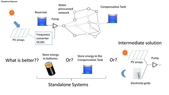
:Photovoltaic energy production is nowadays one of the hottest topics in the water industry as this green energy source is becoming more and more workable in countries like Spain, with high values of irradiance. In water pressurized systems supplying urban areas, they distribute energy consumption in pumps throughout the day, and it is not possible to supply electromechanical devices without energy storages such as batteries. Additionally, it is not possible to manage energy demand for water consumption. Researchers and practitioners have proven batteries to be reliable energy storage systems, and are undertaking many efforts to increase their performance, capacity, and useful life. Water pressurized networks incorporate tanks as devices used for accumulating water during low consumption hours while releasing it in peak hours. The compensation tanks work here as a mass and energy source in water pressurized networks supplied with photovoltaic arrays (not electricity grids). This work intends to compare which of these two energy storage systems are better and how to choose between them considering that these two systems involve running the network as a standalone pumping system without being connected to electricity grids. This work also calculates the intermediate results, considering both photovoltaic arrays and electricity grids for supplying electricity to pumping systems. We then analyzed these three cases in a synthetic network (used in earlier research) considering the effect of irradiation and water consumption, as we did not state which should be the most unfavorable month given that higher irradiance coincides with higher water consumption (i.e., during summer). Results show that there is no universal solution as energy consumption depends on the network features and that energy production depends very much on latitude. We based the portfolio of alternatives on investments for purchasing different equipment at present (batteries, pipelines, etc.) based on economic criteria so that the payback period is the indicator used for finding the best alternative, which is the one with the lowest value.
1. Introduction
One challenge for water pressurized network (WPN) managers is the efficient management of water and energy (both scarce resources). The water scarcity problem will be more serious due to the increase in population and the water demand will be 70% higher for the year 2050 [1]. Although practitioners know this water scarcity problem well, the energy problem is not a minor issue. In 2016, the International Energy Agency [2] stated that energy use in the water sector in 2014 was equivalent to 4% of global electricity consumption. Europe has similar numbers, with 3% of global electricity consumption [3], and other studies on efficient and low-carbon energy consumption have been carried out worldwide [4,5,6,7,8]. In Spain, the water sector consumed 5.8% in 2008 [9], but the authors did not include Spanish households in the primary energy consumed.
In this scenario, with high pressure on the environment, solar energy has emerged as an alternative for energy and emissions reduction. Standalone photovoltaic (PV) systems have become one of the hottest topics in energy production in Spain because of changes in legislation to eliminate taxes linked to energy obtained from sunlight and the price drop in solar panels. Researchers have carried out many projects in optimizing the use of PV systems in general (production, storage, scheduling, etc.) [10,11,12,13]. Additionally, their use in irrigation networks has been explored [14,15,16] because of their energy consumption reduction [17,18]. Some approaches have focused on standalone direct pumping photovoltaic systems without storage systems [19,20], on solving the shadows passing over the generator [21], on investigating the effect of variable solar radiation on a PV based system [22] and on coupling irrigation scheduling with solar energy production [23]. A tool to synchronize the energy produced and the energy required in an irrigation network while minimizing the number of photovoltaic solar panels was developed [24], which requires that operators control the water and energy demand to fit the energy required by crops to the energy produced by photovoltaic (PV) panels. Some other approaches have calculated the life cycle of a PV system considering the environmental and economic impact sources for rural irrigation systems [25] and the energy payback time and greenhouse emissions [26]. Although operators cannot control the water demands in urban WPN as they do in irrigation systems, this did not avoid the use of photovoltaic technology to supply pumping devices in many regions of the world such as the USA [27,28], India [29], Finland [30], Brazil [31], Malaysia [32], and Spain [33]. In areas with high potential (semi-arid regions and high irradiation levels), many practitioners implement this technology for sizing PV systems [34,35,36,37], minimizing the number of PV modules [38], optimizing the tilt angle [39,40], and comparing the environmental and economic impacts of supplying pumps with electricity grids or PV cells [41]. Photovoltaic systems may influence the voltage quality in electricity grids [42], affecting the voltage profile and harmonic distortion of the current and voltage, although some customer-side energy storage systems can make voltage management more economical [43], we proposed using the energy produced in pumping devices that may work as a standalone system. Economic prioritization for the PV installation alternatives has been proposed [44] for minimizing the payback period (period required to recoup the funds invested). We can use this method in urban WPNs to find the best alternative when the utility manager is planning a PV system to feed pumping devices. Nowadays, the utility manager does not know which is the best choice between two common alternatives: batteries or a compensation tank as energy storage. Water pressurized networks were designed without considering tanks in the optimization process, but researchers and practitioners have made an effort to integrate them and optimize their size [45,46,47,48] in real-world operation projects. Tanks are of paramount importance in WPNs [45] because of their use as water storage (filled during the day while it empties, releasing the volume at night) for daily use and in emergencies, but they present inconveniences regarding higher water age and higher energy consumption [49], and some approaches have considered the effect of tanks in the indirect water supply [50]. Recent works highlight batteries as an environmental alternative [51,52,53] in many types of standalone PV systems [54], to concentrate the solar energy to a higher power, and to solve irregularities in the solar irradiation [55]. Some approaches have also analyzed PV hybrid solutions (the electric power grid vs. diesel and photovoltaic generators) [56].
This work compares an urban WPN current state (Case 0; pumps powered by electricity grids) and the new scenarios reached if PV arrays feed pump devices. We converted the urban WPN into a standalone direct pumping photovoltaic network with energy storage in batteries (Case I) or in deposits (Case II). To compare these scenarios, we assessed the energy savings on hydraulic models to calculate the response of each alternative and calculate intermediate solutions (Case III), where PV arrays supply pumps during daylight and electricity grids at night. We planned this problem as a discrete optimization problem, and the lowest payback periods are the most effective option.
The limitations of this study are that it requires a calibrated hydraulic model, which represents an urban WPN meeting the quality and pressure service standards [57] in EPAnet [58], although the calculation in some other hydraulic solvers is also possible such as WDNetXL [59], Infoworks, etc. We calculated the energy consumption in the WPN with UAEnergy software [60], and with the energy efficiency of the pump, we calculated the energy savings and variable costs linked to energy [61]. Some other restrictions appeared in the optimization problem as energy production varies monthly, so the compensation tank should have sufficient volume to avoid overflows, and water should be delivered to meet the quality and pressure standards (hydraulic restrictions).
We rest of this paper is organized as follows. Section 2.1 shows the formulas used for calculating energy production and its variation. Section 2.2 analyzes the key features arising if storing energy in deposits, Section 2.3 quantifies the energy savings calculations, and Section 2.4 describes the return on investment calculation. Section 3 presents the optimization problem while Section 4 performs the synthetic case study. Section 4.1 presents the input data and Section 4.2 shows the step-by-step results, Section 4.3 the discussion section, Section 4.4 perform the sensitivity analysis and Section 4.5 outlines the future developments. Finally, Section 5 shows our key conclusions.
2. Materials and Methods
2.1. Monthly Variation in Energy Produced in Photovoltaic Arrays
Some approaches have outlined [29,62] the variation of the solar global reaching the Earth’s surface and the latitude as one of the most common parameters. We considered this variation with the equations described in [63] to calculate the energy production for a single PV panel.
Water and energy consumption are also variables influenced by water use (outdoors, swimming pools, etc.), temperature, and precipitation as well as neighborhood [64]. Following these ideas and being aware that freshwater scarcity is a growing concern [65], we modeled the water consumption considering the usual water demand multiplied by a constant (K; with monthly variation) to incorporate the higher consumption during summer.
Considering the water–energy nexus, higher water demands (during the summer) involve higher energy demands and higher energy produced by PV arrays (also in summer). Likewise, the months of lower water consumption (December, January and February) also correspond to those of lower photovoltaic electricity production. It is not possible to select the most unfavorable month before performing every calculation, regardless of whether it is December, which is the worst (lowest irradiation and energy production), or July (higher water consumption and energy production), or some other month. However, we could understand this after the hydraulic analysis performed here and as it considers WPN characteristics, it does not have a universal response.
2.2. Energy Storage in Tanks
Indirect supply using tanks as water storage has a key advantage as tanks guarantee reserves for emergencies. In the present approach, we also considered tanks as an energy storage system. The major limitation of the energy supply with PV arrays is that sunlight (irradiance) limits the number of operating hours of the pumps (6–9 hours depending on the latitude of the WPN). Equation (1) helps to calculate the volume stored to guarantee supply at nights ():
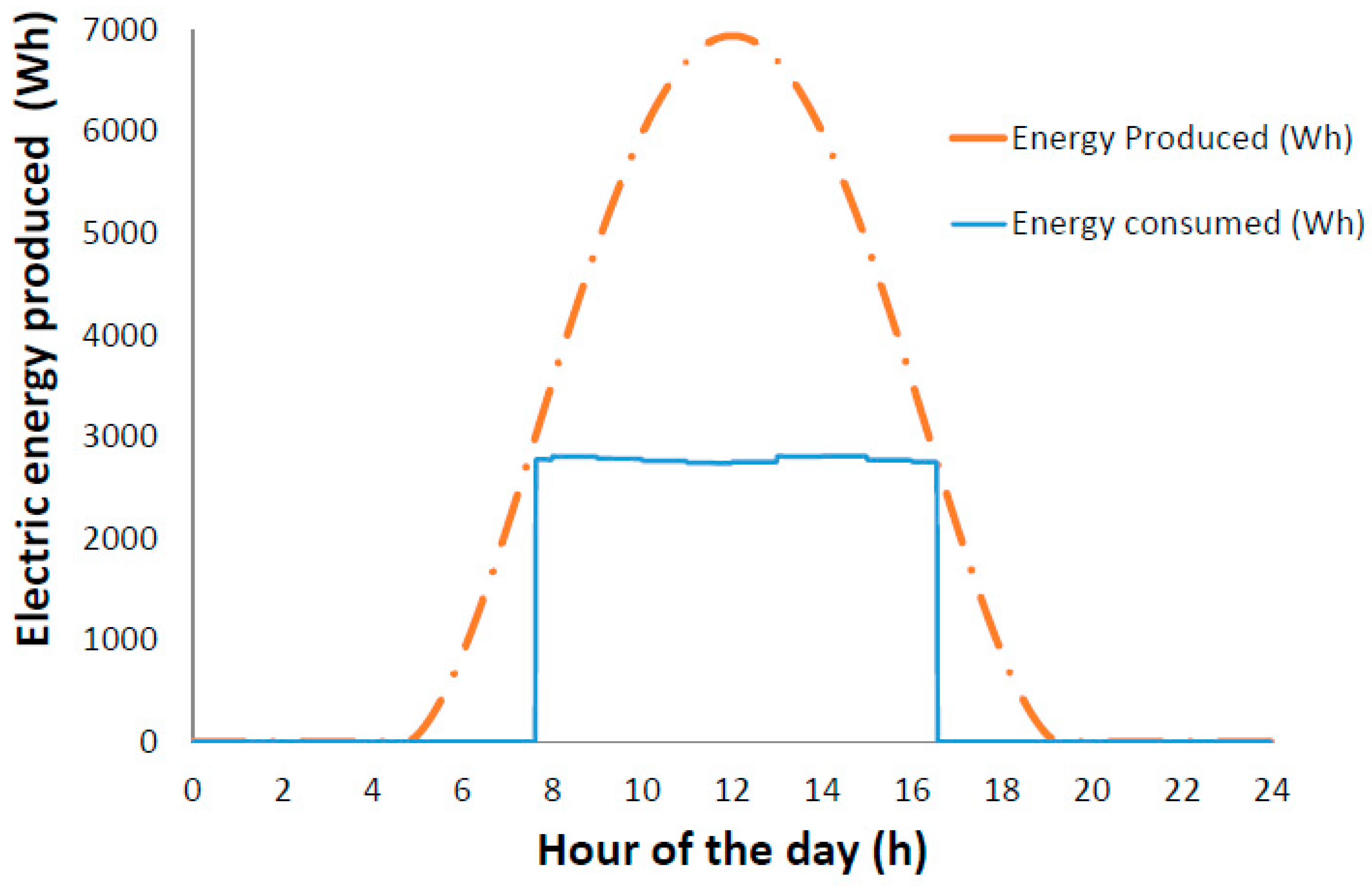
where is the city daily water demand and the volume consumed when there is sunlight and the PV arrays are supplying electricity to the water pumps. Figure 1 shows a typical situation as the water pumps have eight hours to fill the tank and the energy should be lower than that of the energy production (stripped line).
In many urban WPNs, it is essential to enlarge the compensation tank to store these amounts of water. The need to fill the tank in these irradiance hours should involve over-sizing some pipelines and adding some new pumping devices. We should consider all these infrastructure costs as investments performed in the initial year (I0).
2.3. Non-Renewable Energy Savings
We defined and divided the final price of water into fixed and variable costs [61]. The variable cost of water may depend on the water cost itself (economic cost of the source in its raw state, not relevant as the cost of the water delivered must be the same to allow comparison), the energy cost (electricity supplied by grids or by the photovoltaic process), and useful life of the infrastructure (pipelines, pumps, PV arrays, batteries, etc.).
This new energy source involves saving non-renewable fuels (coal, oil fired, nuclear). The economic savings expected in standalone PV direct pumping in WPNs should be the electricity costs as PV panels will produce the energy demanded. We expect lower savings for intermediate solutions where PV panels provide energy during daylight and electricity grids for the rest of the day.
2.4. Economic Prioritization of the Alternatives
Economic prioritization involves solving an optimization problem where the indicator used for getting the prioritization scheme is the payback period [44] (Equation (2)).
where Ti (years) is the payback period (value to minimize as lower values involve higher water and energy savings per monetary unit invested); r is the equivalent continuous discount rate [66] used for expressing future savings in monetary units at the present time; I0 is the investment performed in year 0; and Si is the economic savings.
The utility manager needs to analyze whether it is better to use batteries or tanks for energy storage or an intermediate mixed solution combining energy supplied by PV arrays and electricity grids. In this analysis, the decision-makers must make investments now to gain future revenues (energy savings; cumulative cost). We calculated the payback period to compare the alternatives, with the lowest value being the best alternative.
3. Optimization Problem
3.1. Input Data
In this section, the input data were divided into Hydraulic, Irradiance, and economic data.
3.1.1. Irradiance Data
We divided the data required to calculate the irradiance and to obtain the energy availability into those showing and those not showing monthly variation. The first ones (monthly irradiation data) are global irradiance on a horizontal surface (H), average temperature (), and the representative day of the month (n). The constant data are the angle of inclination of the photovoltaic panels (β), the solar constant (), the irradiance under standard conditions (), the performance decay coefficient because of the rising temperature of the cell (), the cell temperature under standard test conditions (), the latitude angle (φ), the albedo (ρ), the peak power generated by the PV modules (PP), the asynchronous motor efficiency (), and the converter efficiency ().
3.1.2. Hydraulic Data
The optimization problem requires some hydraulic data to obtain the energy consumed by the WPN. The water (and energy) demanded by population represents values not modifiable by the utility manager and only dependent on population, temperature, month, etc.
The hydraulic data required here are:
- The hydraulic model of the network. This is the calibrated and operative model that accurately represents the hydraulic behavior of the WPN; no errors should appear when running it. This file must contain the elevation, base demands, and temporal variation in nodes, and the roughness, diameter, and lengths in pipes. It should also consider the pump curves and size of the tanks.
- Pump efficiency (). We highlight this parameter since its use produces a closer approach to reality.
- Monthly water demand variation (K). We should obtain this parameter by dividing each monthly water demand into the average water demand. Their values should be close to 1.
3.1.3. Economic Data
It requires these economic data to calculate the payback period for every alternative considered in the WPNs. The economic data have been already displayed in Equation (2). The full explanation is the following:
- Equivalent continuous discount rate (r).
- Current investment (I0). This value is different depending on the alternative analyzed, but any of them represent the proper characteristics of every case analyzed. Although the PV arrays costs are similar for every alternative considered, if the battery is operating, we included this cost in the calculations and if tanks are the device selected for storing energy, we incorporated the cost of increasing the tank capacity, new pumps, and pipelines and any other devices to meet the hydraulic demands.
- Economic savings (Si) for every alternative in comparison with the current case (Case 0). To calculate the energy consumption costs, we used the Spanish tariff (which involves calculating power, energy, and reactive energy with different hourly values and the seasonal variation).
3.2. Calculation Process
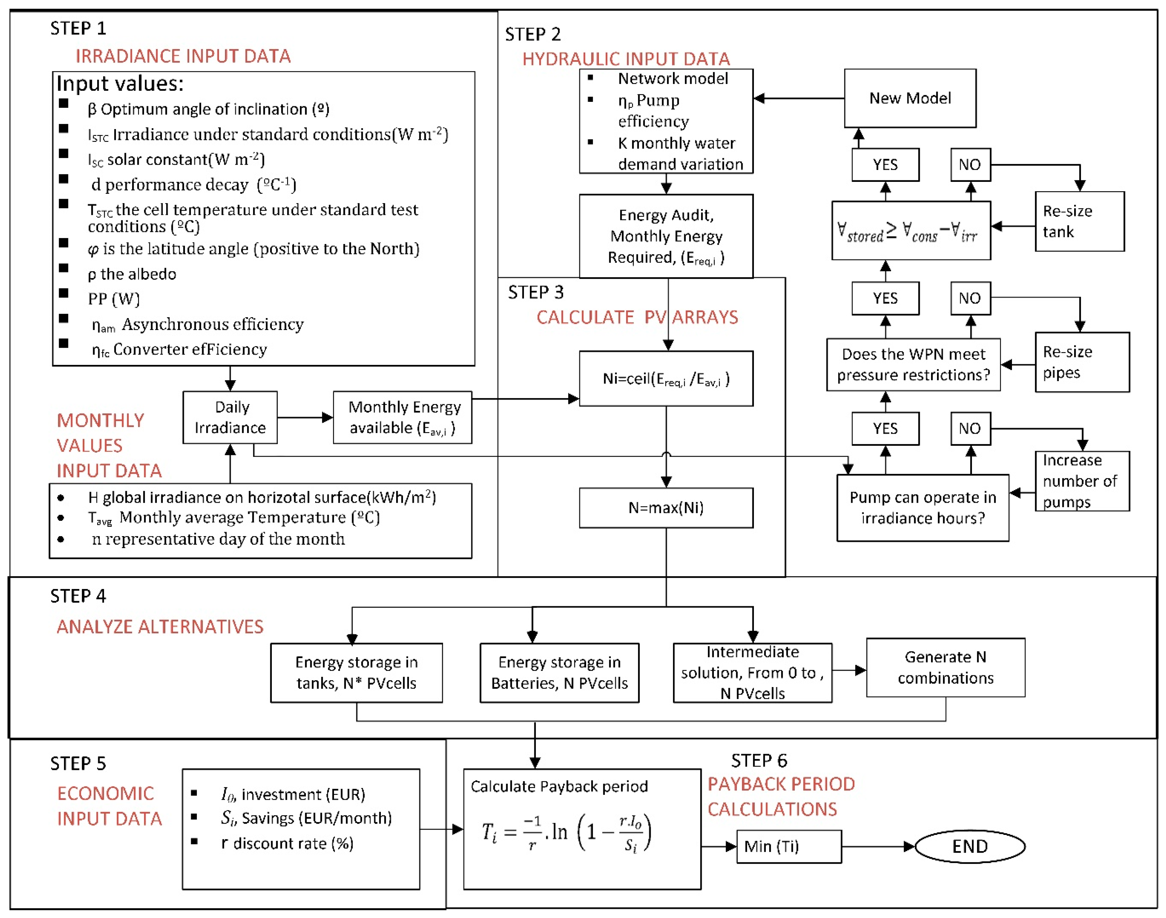
Figure 2 reproduces the calculation process designed in six stages. First, we calculated the monthly energy available (Step 1). With the daily solar duration data from Step 1, we can study the needs (pumps, pipes, increased volume of the tank, etc.). Additionally, we calculated the energy needed for the present case (Step 2). With the results obtained in Steps 1 and 2, we calculated the number of PV panels, N (Step 3), and we designed three cases (Step 4).
The latest case (the WPN operates by getting energy from the electricity grids) incorporates N potential schemes, each of them with several PV panels installed ranging from 0 to N.
In Step 5, we quantify the investments and savings for the scenarios represented before, and we determine the payback period for every scheme in Step 6.
Step 1: Calculation of the monthly energy available per PV panel and the hourly irradiation for every month.
Step 2: Calculation of the monthly shaft work required by the pumps in the WPN.
With the hourly values of irradiation, the utility manager should count if the pump may elevate the whole amount of water to the compensation tank, if the pipeline diameters are adequate and if the compensation tank capacity is big enough to allow for the new operation plan. As shown in Figure 1, pumps can only work within the central hours of the day and the compensation tank must not be exceeded (water is a valuable resource) nor the tank emptied (air would enter the WPN).
Step 3: Calculation of the number of PV arrays.
We considered that the minimum number of solar panels matching the constraint energy available (produced) must be greater than the energy required by the WPN at every moment of the day [24]:
where is the i-th value (being i a month) for the unitary energy available (Step 1) and is the i-th value for the energy available (Step 2). The quotient is the number of solar panels to meet the i-th water demand for every month studied. This is a 12 × 1 vector that shows the number of PVs necessary for every month. The greatest of these 12 values results in the number of solar panels required.
We calculated the total of solar panels () considering the electricity consumed by the city and electricity produced by the PV arrays. This collection does not depend on energy storage (tanks or batteries). This value is the upper threshold () for the intermediate case. If we produce more energy, the WPN may work disconnected from the electricity grids.
Step 4: Description of alternatives.
The first alternative is to accumulate the energy in batteries, and the second alternative is to store the energy in tanks. These options involve as many PV panels as required to operate as standalone systems (without being supplied by electricity grids). The third alternative involves generating several combinations with a different number of solar panels (varying among 0 and ) for an intermediate solution (during nights, electricity grids supply pumping devices).
Step 5: Calculation of the economic input data.
We calculated the investments and savings for the alternatives described previously (PV arrays, batteries, new pumps, re-sizing pipelines, and increasing the capacity of the tank). In our approach, we did not consider the compensation tank costs (they were very large for the investments analyzed), but other researchers and practitioners can include it for future cases.
In the intermediate alternative, each combination requires different expenses (each combination involves a different number of PV arrays) and in the same way, the savings (the more energy production is the less energy consumed by electricity grids).
Step 6: Calculation of the payback period for the alternatives.
Finally, the minimum payback period, the most economical alternative and selected for implementation with Equation (2).
4. Case Study
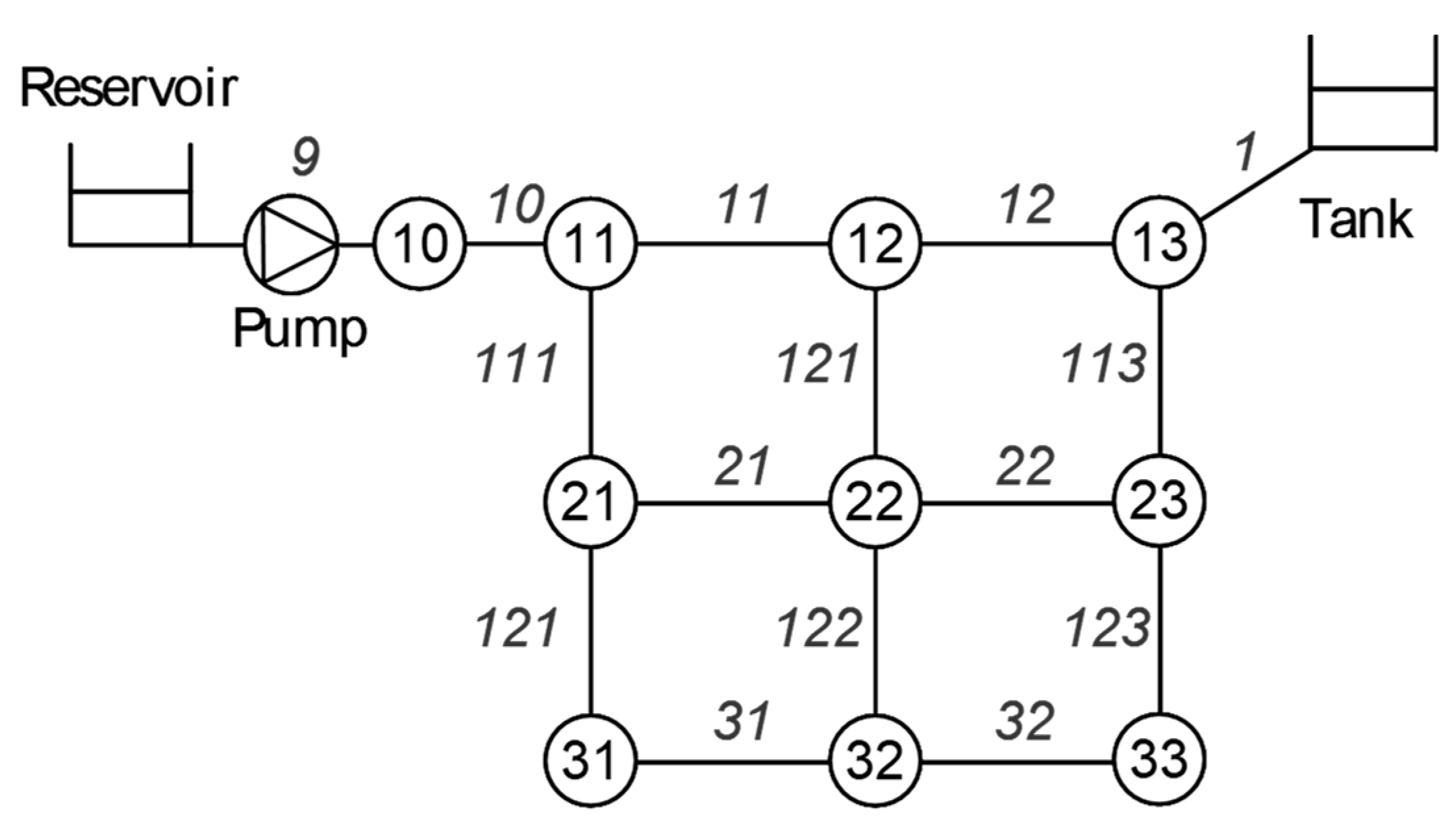
To illustrate the proposed method, Figure 1 shows the case study analyzed here (latitude φ = 39.47° N and longitude 0.3747° W). Line and node data, demand pattern multipliers, etc., can be found in [67] and in Supplementary Materials. We proposed Case 0 as the current state of the WPN where the pumps are supplied by electricity grids and they start and stop working controlled by the tank level.
In Cases I and II, the PV arrays supply the whole energy demanded by the pumping devices in the WPN. Case I includes batteries that store the peak energy production (at midday) and release this at night, while Case II is the scenario in which we store energy in the compensation tank (Figure 3), feeding pumping systems with PV arrays for the central hours of the day (from 6:50 to 16:30 h). Case II involves pumping the whole daily water consumption in the above central hours of the day. Therefore, we expect to solve the hydraulic restrictions increasing the pumping capacity with pumps operating in parallel, pipe diameters, and the tank capacity (now it should be able to store a higher volume of water).
Finally, Case III is the intermediate case in which we installed PV arrays as energy support during daylight, but we supply the pumps at nights through electricity grids.
4.1. Input Data for the Case Study
In order to increase readability, input data were classified following the guidelines described in Section 3.1.
4.1.1. Irradiance Input Data
We calculated the monthly energy production produced in PV arrays using the [63] equations, and Table 1 shows the data required (described in Section 3.1.1).
Some data vary with the month as the monthly average temperature () and the day of the representative month (n coefficient, the value that highlights monthly energy production variation [63]) is shown in Table 2. Due to the measurements performed by the flowmeter installed in pipeline 10, we included the monthly variation of the city water demand. A multiplier K on the average water demand of the consumption nodes (domiciliary uses) is depicted in Table 2.
4.1.2. Hydraulic Input Data
The hydraulic data required are the WPN model (which includes elevation, base demands, and temporal variation in nodes, and roughness, diameter, and lengths in pipes). The pumping system consists of Ebara pumps, model GS-1450 rpm (ref. 623GS33048294) [68], and characteristic curves ; (H in m, Q in L/s). It maintains every consumption node with pressures above the minimum threshold pressure (22 m). Pipe roughness was equal to 0.1 mm, the diameter of the compensation tank was 20 m, and its level oscillated between 2.5 m (initial value for the simulation) and 7 m (maximum value).
4.1.3. Economic Input Data
The investment to install the PV panels (1.6 m2; an input data that depends on the PV panels selected), batteries, pipelines (numbers proportioned by a water utility operating in Spain), etc. is depicted in Table 3. The equivalent continuous discount rate is r = 2%.
We calculated the economic savings considering the 3.0 Tariff. These costs depend on three components (power in kW, active energy in kWh, and reactive energy in kVArh) as well as hourly (peak, plain, and low) and seasonal variations (winter and summer otherwise). Every detail is shown in Table 4.
Regarding the useful life of the infrastructure, 25 years is the value selected for the PV arrays and pumps devices, while five years was for batteries and 50 years for pipelines. Standalone direct pumping photovoltaic systems represent high revenue as it eliminates fixed costs related to the use of electricity grids.
4.2. Results
4.2.1. Monthly Energy Production by PV Arrays
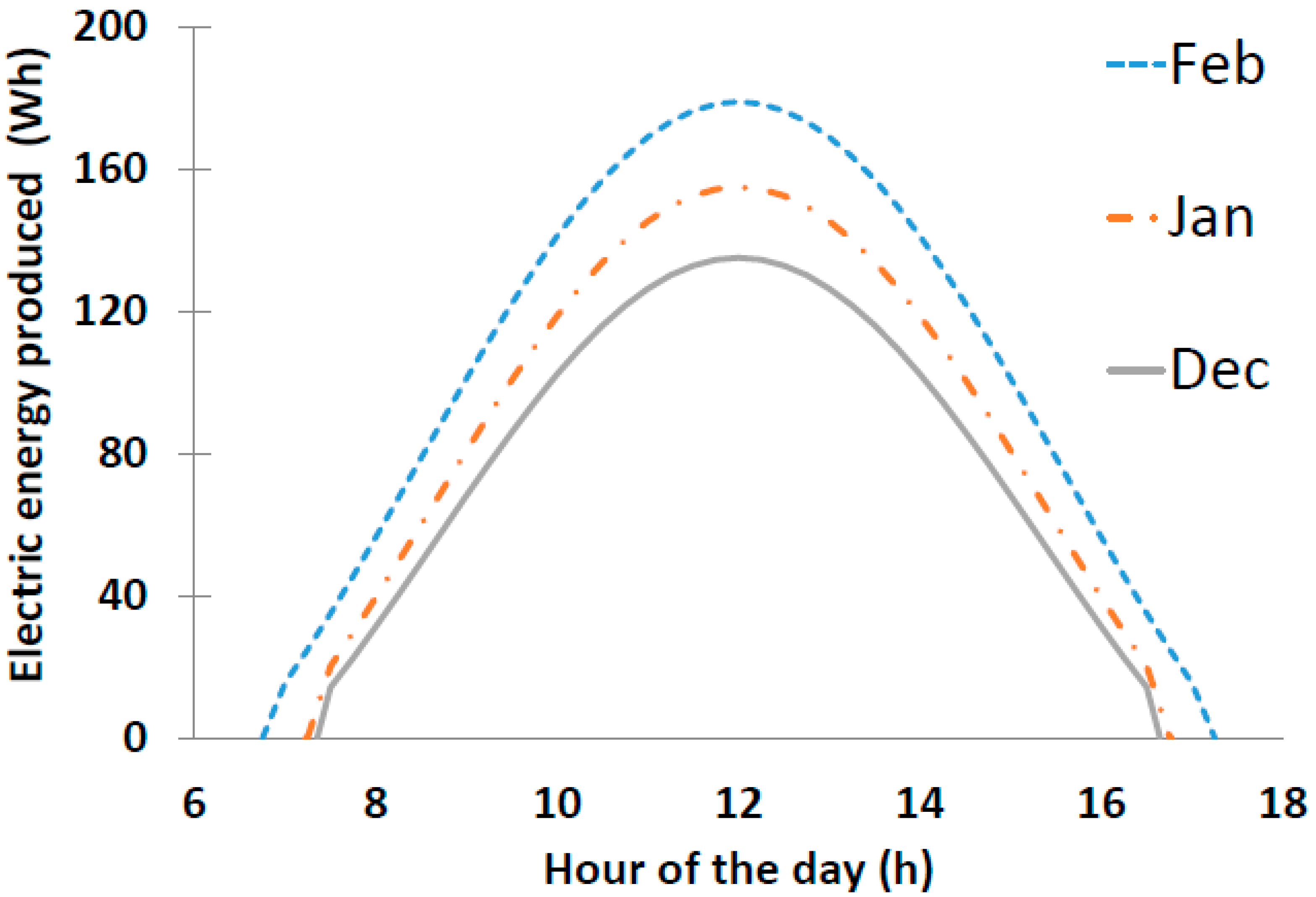
Figure 4 depicts the irradiation curves for the three months with lower irradiation (January, February, and December) for a single PV array and Table 5 shows their numerical values. It is not possible to select the most unfavorable month a priori because water consumption is not constant (a constant K considers this variation, Table 2). If December is the worst, we could confirm this after the hydraulic analysis performed in the following section.
4.2.2. New Model Generation for Energy Storage in Tanks (Case II)
We calculated the city daily water consumption ∀cons = 3326.40 m3 (Case 0) and the volume consumed when there is sunlight (values that vary every month that were in the previous Section 4.2.1; Figure 4) = 1538.46 m3. When the sun goes down, water stored in the tank should be higher than these two figures (in Equation (1)) m3. With the tank dimensions presented in case 0, we calculated the maximum volume stored 1413.72 m3, a value that we should increase to meet in Equation (1). Finally, we enlarged the new tank diameter up to 30 m and the tank capacity was great enough to allow for water supply during the night.
The pumps must supply the whole amount of water (3326.40 m3) in 8–10 h, which means greater flow rates (and head losses) than those planned when dimensioning this WPN. Using three pumps running in parallel increases the flow rates, and resizing pipelines reduce head losses (new diameter for pipelines 10 and 11 are 350 and 300 mm; Figure 3). The decision of selecting a different number of pumps, increase in other pipeline diameters, and enlarging the tank dimensions are not the key point of this study, that is, to analyze the new WPN (Case II), which may work disconnected from the electricity grids.
4.2.3. Monthly Energy Consumption and PV Arrays Calculation
UAEnergy [60] calculates the monthly energy consumption and the third and fifth column of Table 5 shows the average daily energy consumed in Case I and Case II. UAEnergy returns the shaft work required by the pumps, and we considered here the effect of the pump efficiency to obtain the electricity demanded by the system. Once we calculated the monthly energy consumed and the energy produced, the number of arrays to supply the WPN can be calculated using Equation (3).
Case II shows a higher energy consumption (as pumps are only operating at the irradiation hours), which involves high flowrates and high energy dissipation in friction and consequently leaves no room for surprise. The higher the energy, the greater the number of PV panels.
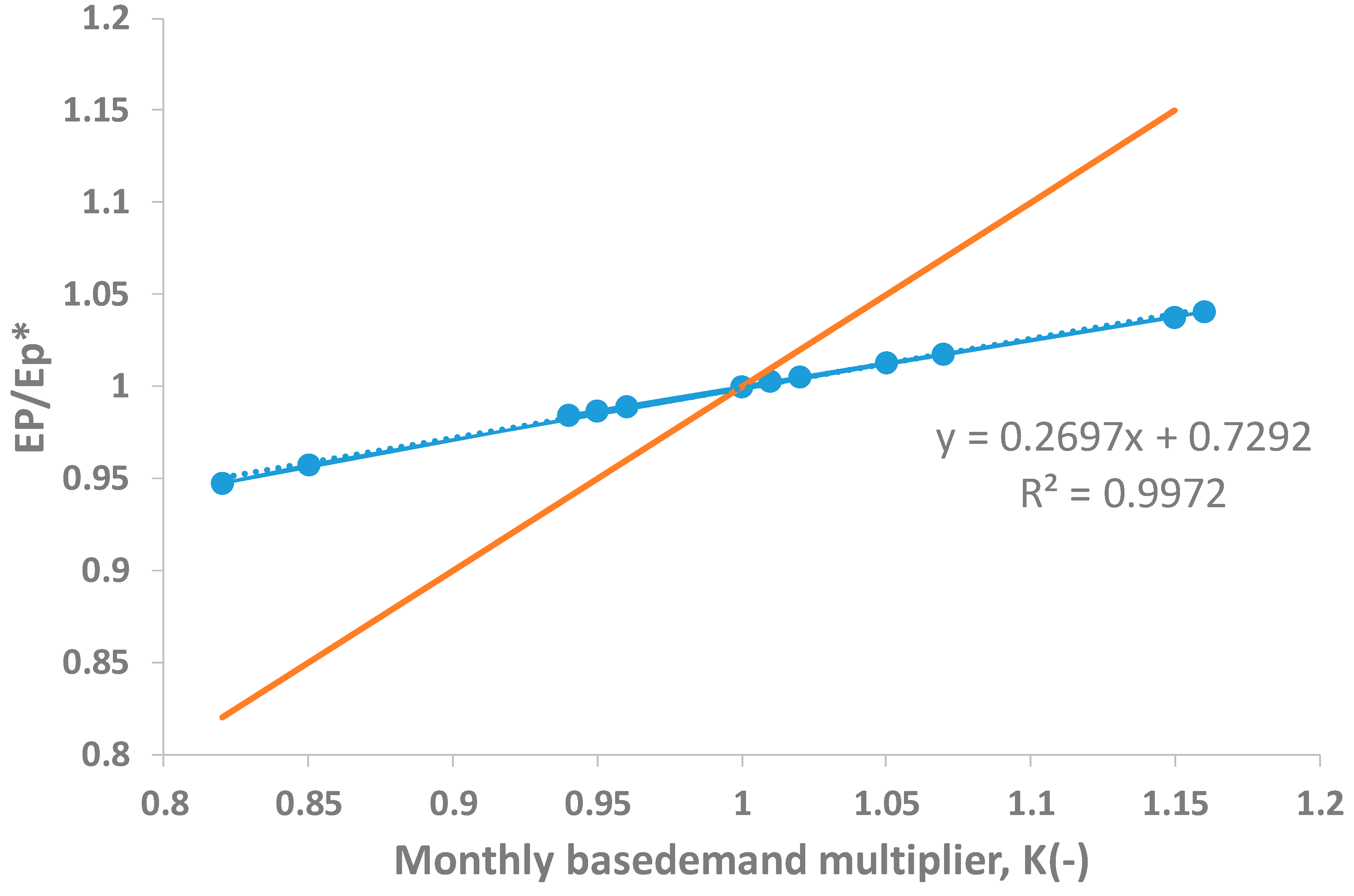
The quotient between energy consumption for every month (different values of K(-), dimensionless; Table 2) and energy consumption for a month with the value K = 1 (October) has been calculated. Figure 5 shows the values calculated per every month (different values of this K parameter), and it may be observed that a base demand variation of 15% involves in our case study a lower variation in energy consumption variation (4%); a result that highlights the fact that energy consumption in our WPN is more sensitive to energy production than by water consumption.
4.2.4. Investments and Energy Savings for the Analyzed Cases
In Case I, PV arrays to carry out at year 0, and the batteries (the batteries’ lifetime was assumed to be five years) in years 0, 5, 10, 15, and 20. As the I0 (PV panels = 1000, Table 5) and Ibat values have already been presented, the investment in EUR from the present time —tp—should be = 359,480 + = 631,509.23 EUR.
In Case II, the PV arrays, re-sizing pipelines, increasing the number of pumps and increasing tank capacity represent the investments to address in year 0. = 433,892.36 + 79,040 + 33,340 + 2 × 10,136.5 + 215,984.49 = 782,529.85 EUR.
In Case III, we can calculate the investment with the value of the PV installation. The costs in the present year are: .
Energy consumption in Case 0 is the energy savings for Cases I and II (standalone systems). Therefore, these figures are the same for both cases (Table 6) as they are standalone WPNs. In Case III, we kept the WPN connected to the electricity grids and PV arrays’ supply energy during daylight. Thus, the economic savings only affect the energy term (other terms such as power stay constant). With these constraints, we calculated the energy savings for the alternatives (in this case, 1000 alternatives). Some of these economic savings (with 100, 300, 500, 700, and 900 PV panels) are shown in Table 6.
4.2.5. Payback Period Calculations
The payback period calculation (Equation (2)) for Cases I and II returned the numerical values of 6.99 and 8.82 years, respectively. As both have the same economic energy savings, the lower the investment, the lower the value of the payback period.
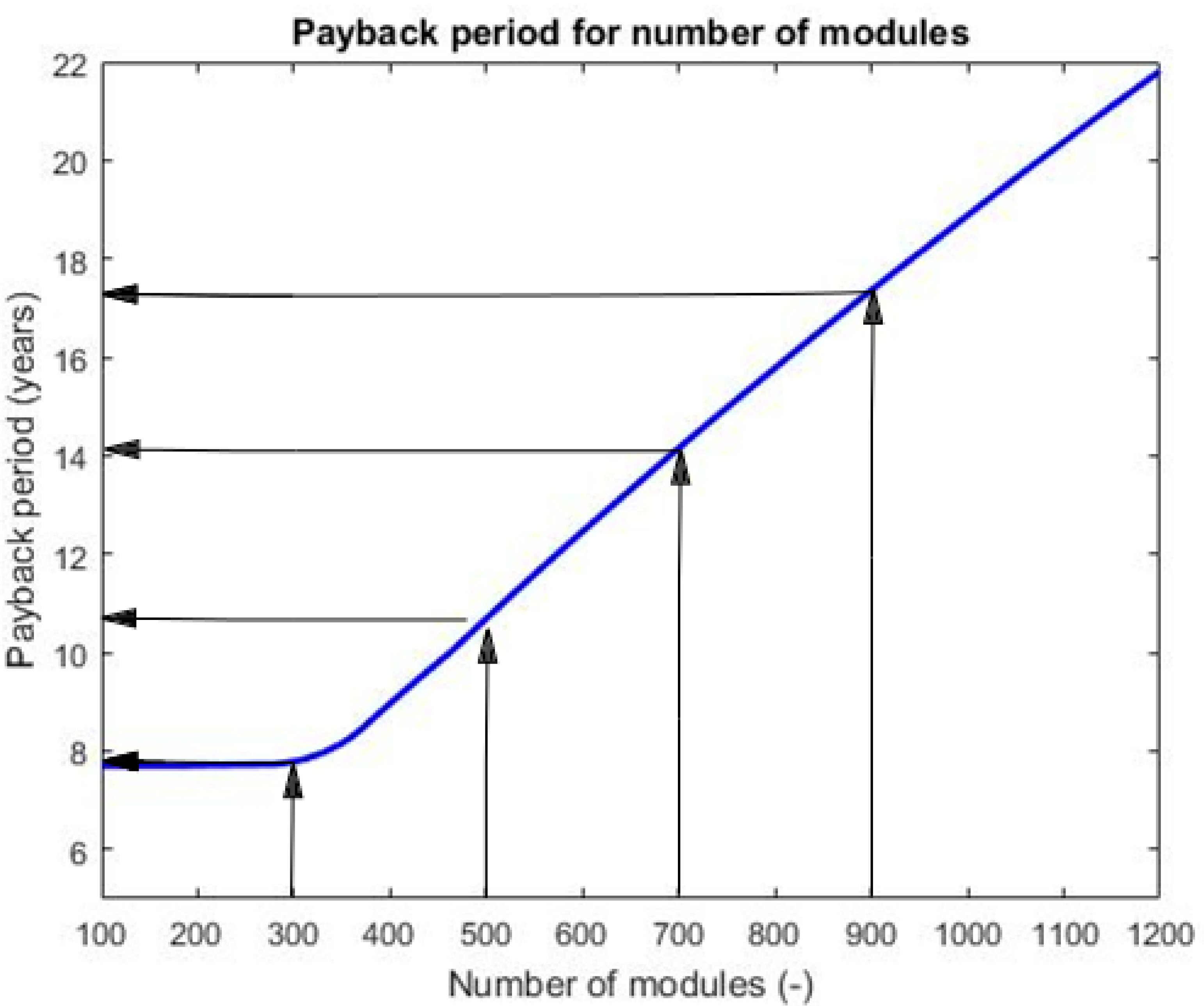
To understand the potential payback periods for the huge (although finite) possibility of installing between 0 and 1000 PV panels, we computed these possibilities showing the values shown in Figure 6 (the abscissa axis is the number of modules, a dimensionless value represented by (-)). The results show that for a wide range of PV panels (0–310), the pumps consumed the whole energy supplied. Therefore, every panel involved constant energy saving, but for higher values, the pumps cannot consume the whole energy produced (in peak hours of the day, it produces more energy than required by the WPN) and because of that, new PV arrays result in lower energy savings.
4.3. Discussion
For clarification, we summarize the essential aspects of the method proposed and the case study developed in this section. In general terms, using renewable energies (PV arrays) is more convenient than conventional electricity supply through grids. However, three key uncertainties make it difficult to obtain the right calculation to justify the investment needed for the transition: quantity and variability of water consumption, size and variation of solar irradiation, and features of the water distribution network (layout, sizing, pumps, etc.).
The data to carry out the calculations for this assessment are not a problem, since information on solar radiation, water consumption, and network composition is available (the data required were described in Section 3.1). The practical problem deals with the procedure for performing these calculations, and this is the task resolved by the method we present here. We should remark that the whole method is available and described here, is UAEnergy, a free MATLAB-based educational software (source codes available in [60]) developed to compute the energy audit of WPNs.
The case study aims to illustrate this. Thus, for a supply of 20,000 people, we propose the following cases:
- Case 0 (current): Direct electric supply from the grid (non-renewable energy).
- Case I: Full electricity supply through PV (renewable energy) and energy storage in batteries of the surplus electricity during peak production hours.
- Case II: Full electricity supply by PV (renewable energy) and energy storage in a compensation tank (as potential energy) of the surplus electricity during peak production hours.
- Case III: Electricity supply combining PV (renewable energy) at sunlight hours and direct from the grid (non-renewable energy) at night.
The average water consumption for every case studied was 3326.40 m3/day (being +18.38% in July and −24.42% in February). The yearly average energy production per single PV array was 1402.73 kWh/day (the peak in July was 1990.96 kWh/day and the lowest value was 791.49 kWh/day in December).
In Cases 0, I, and III, the average energy consumption was equal to 813.20 kWh/day (the greatest and the smallest energy consumptions were 886.16 kWh/day in July and 734.94 kWh/day in February). In Case II, these figures were 960.67, 977.55, and 941.86 kWh/day. We calculated this with the data provided by Table 5.
The application of the method (Figure 2) allowed us to quantify the key values for each alternative. While Cases I and II showed various investments (described in Section 4.2.4), Case III incorporated a high number of cases (a finite number ranging from 0 to the minimum number of PV arrays for other cases analyzed). We computed the cost savings with the Spanish 3.0 tariff. In Cases I and II, we saved the electricity before it was consumed (in the current state, Case 0), but in Case III, we saved a smaller amount of energy as the system worked as a hybrid solution combining renewable energy and electricity from the grid. We summarize these in Table 7.
In this case study, it turns out that energy storage in batteries resulted in the best solution (the minimum payback period). However, aforementioned, this was not relevant, but the method. This work highlights that Cases I and II returned the most non-renewable energy savings (and emissions) and Case III showed an intermediate scenario that was much more favorable for the number of PV panels below 250 (when the number increases, every new panel results in lower savings and consequently a higher payback period, Figure 6).
4.4. Sensitivity Analysis
We considered the equivalent continuous discount rate as a sensitive parameter ranging from 0% to 4%. It compares the present value of money in its present value to the future considering real interest rate and deflation. Although this value is not modifiable by water utility managers, we illustrate its influence in Figure 7.
The results bear no surprise as the smallest discount rate involves the least depreciation of future money, and it encourages utility managers to make investments (we obtained lower values of payback periods). As we obtained the same economic savings in Cases I and II (and the equivalent discount rate is a fixed term imposed by depends on the national banks in each country), the payback period is only influenced by expenditures, and the lowest investment gets the smallest payback period. In other cases, energy storage in tanks could be a more workable option.
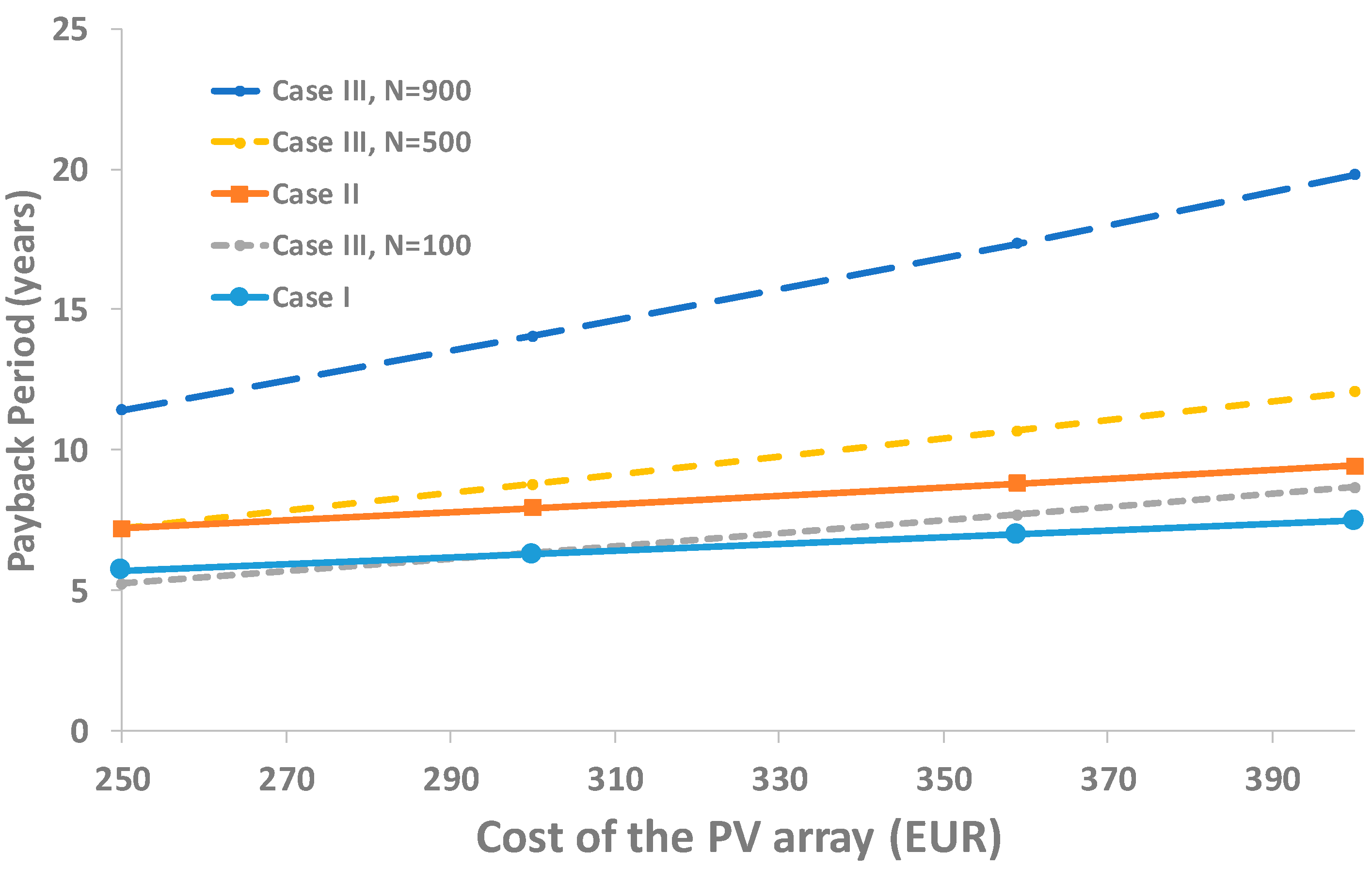
To consider the current scenario in Spain, where the price of PV arrays is decreasing, we calculated this effect and depict it in Figure 8. The results showed that the combination alternative (Case III) may become the selected choice for a few PV panels. We can state that hybrid solutions are more efficient if the number of panels are low as it is better to work the WPN as standalone direct pumping systems for a higher number of PVs. The rates shown here indicate that these procedures are feasible nowadays and utility officials should incorporate them when managing WPNs.
4.5. Future Developments
This study required a calibrated hydraulic simulation model to solve the hydraulics in a WPN, a programming software (MATLAB®, Visual basic, etc.) running in a PC, and the input (hydraulic, irradiance and economic) data aforementioned. We cannot use this method in gravity-fed towns (they do not need pumping devices) and in WPNs without a compensation tank, we could not undertake Case II analysis.
The results of the method described here applies to society. It processes a daily non-renewable energy savings of 1402.73 kWh/day. Therefore, we expect to use this method in many urban WPNs in the Alicante province, those managed by the Diputación de Alicante. It is important to highlight the variation in many towns that arises from the network layout and other features and the current method will show the best choice in each town (not expected to be similar in every town).
We submitted a project to the Ministry of Spain in his last call “Knowledge Generation and Scientific and Technological Strengthening of the R&D&i System”. This project involves building a pilot plant of a standalone PV pressurized irrigation network, where we can manage the energy demand. This project belongs to a scenario of a future irrigation network (we used reclaimed water to irrigate crops) with zero water, zero energy, and zero emissions (called “neutral water” and in this case, “neutral energy” and “neutral emissions”). We expect to obtain experimental data at this pilot plant and to represent similar projects in other regions with which to multiply the effect of such implementation.
5. Conclusions
This work deals with converting an urban WPN (with pumps supplied by electricity grids) into a standalone direct pumping photovoltaic system. Utility managers are facing this opportunity as photovoltaic panels have become an environmental and workable alternative to traditional energy supply, and they represent an alternative to avoid overload in electricity grids. As water and energy demands vary at every hour of the day and sunlight providing energy to PV panels only occurs during daily hours, there must be a storage structure that accumulates energy during the day and releases this energy during the night. The utility manager must know the energetic implications of storing energy in tanks or batteries while running the installation isolated from electricity grids.
This problem can be misleading without considering the effect of the monthly variation in irradiation and energy consumption. Energy production in PV arrays and the water demanded by city customers (and energy demanded) are variable terms. When energy consumption is high (in summer), it is also energy production and it is not clear as to which is the most favorable and/or unfavorable month.
This manuscript presents a calculation method that allows any urban WPN to be adapted into a standalone photovoltaic direct pumping system with energy storage in reservoirs or batteries. This method considers how to include these influential factors in reaching the right result. Practitioners may know the best choice of storing energy in batteries, tanks, or an intermediate solution maintaining the connection to electricity grids.
In particular, the method was applied to an urban WPN with real data. As shown, we found that energy production was more dependent on variation than energy consumption in a WPN, with December the most unfavorable month for this study. Battery storage systems have proven to be the most efficient alternative for the cost analysis performed with the lowest payback periods, but many utility managers preferred tank storage systems as a guarantee for supply. The tank alternative is more energy-hungry than the others (Table 5), as the pumping devices should fill the compensation in a short time (those with irradiation necessary to allow the pumps to work). As Cases I and II obtain the same economic savings, we get lower payback periods with lower investment performed.
Between these two alternatives, it provides an intermediate solution that involves being connected to electricity grids and supports provided by PV arrays in the irradiance hours. These combinations (ranging from 100 to 1000 PV arrays) highlight that we get lower economic savings than in the other two cases (as the utility is still paying the electric company). The threshold value, in which the number of PV panels the WPN cannot consume the whole energy produced, is obtained because of the calculations (210 in the case study). For greater numbers of PV arrays (the investment remains proportional) but involving lower economic savings, the result is that the payback period increases.
Supplementary Materials
The following files are available online at https://0-www-mdpi-com.brum.beds.ac.uk/2071-1050/12/2/738/s1.
Author Contributions
Conceptualization, M.Á.P. and R.C.; Methodology, M.Á.P. and R.C.; Software, M.Á.P.; Validation, M.Á.P. and R.C.; Formal analysis, L.B.; Investigation, M.Á.P., R.C., and L.B.; Resources, R.C. and L.B.; Data curation, L.B.; Writing—original draft preparation, M.Á.P. and L.B.; Writing—review and editing, R.C.; Visualization, L.B.; Supervision, M.Á.P.; Project administration, M.Á.P.; Funding acquisition, M.Á.P., R.C., and L.B. All authors have read and agreed to the published version of the manuscript.
Funding
This work was supported by the research project ‘‘GESAEN’’ through the 2016 call of the Vicerrectorado de Investigación, Desarrollo e Innovación from the University of Alicante, GRE-16–08.
Conflicts of Interest
The authors declare no conflict of interest. The funders had no role in the design of the study; in the collection, analyses, or interpretation of data; in the writing of the manuscript, or in the decision to publish the results.
References
- Alexandratos, N.; Bruinsma, J. World Agriculture Towards 2030/2050: The 2012 Revision; Food and Agriculture Organization of the United Nations: Rome, Italy, 2012. [Google Scholar]
- International Energy Agency (IEA) Water Energy Nexus. Excerpt from the World Energy Outlook 2016; International Energy Agency: Paris, France, 2016. [Google Scholar]
- Bijl, D.L.; Bogaart, P.W.; Kram, T.; de Vries, B.J.M.; van Vuuren, D.P. Long-term water demand for electricity, industry and households. Environ. Sci. Policy 2016, 55, 75–86. [Google Scholar] [CrossRef]
- Breadsell, J.K.; Byrne, J.J.; Morrison, G.M. Household energy and water practices change post-occupancy in an australian low-carbon development. Sustainability 2019, 11, 5559. [Google Scholar] [CrossRef] [Green Version]
- Watson, K.J. Understanding the role of building management in the low-energy performance of passive sustainable design: Practices of natural ventilation in a UK office building. Indoor Built Environ. 2015, 24, 999–1009. [Google Scholar] [CrossRef]
- Berry, S.; Davidson, K. Zero energy homes—Are they economically viable? Energy Policy 2015, 85, 12–21. [Google Scholar] [CrossRef]
- Wittenberg, I.; Matthies, E. Solar policy and practice in Germany: How do residential households with solar panels use electricity? Energy Res. Soc. Sci. 2016, 21, 199–211. [Google Scholar] [CrossRef]
- Alghamdi, A.; Haider, H.; Hewage, K.; Sadiq, R. Inter-University sustainability benchmarking for Canadian higher education institutions: Water, energy, and carbon flows for technical-level decision-making. Sustainability 2019, 11, 2599. [Google Scholar] [CrossRef] [Green Version]
- Hardy, L.; Garrido, A.; Juana, L. Evaluation of Spain’s water-energy nexus. Int. J. Water Resour. Dev. 2012, 28, 151–170. [Google Scholar] [CrossRef] [Green Version]
- Cucchiella, F.; D’Adamo, I.; Gastaldi, M.; Stornelli, V. Solar photovoltaic panels combined with energy storage in a residential building: An economic analysis. Sustainability 2018, 10, 3117. [Google Scholar] [CrossRef] [Green Version]
- Zsiborács, H.; Baranyai, N.H.; Vincze, A.; Háber, I.; Pintér, G. Economic and Technical Aspects of Flexible Storage Photovoltaic Systems in Europe. Energies 2018, 11. [Google Scholar] [CrossRef] [Green Version]
- Roncero-Sánchez, P.; Parreño Torres, A.; Vázquez, J. Control scheme of a concentration photovoltaic plant with a hybrid energy storage system connected to the grid. Energies 2018, 11, 301. [Google Scholar] [CrossRef] [Green Version]
- Chen, J.; Li, J.; Zhang, Y.; Bao, G.; Ge, X.; Li, P. A hierarchical optimal operation strategy of hybrid energy storage system in distribution networks with high photovoltaic penetration. Energies 2018, 11, 389. [Google Scholar] [CrossRef] [Green Version]
- Reca, J.; Torrente, C.; López-Luque, R.; Martínez, J. Feasibility analysis of a standalone direct pumping photovoltaic system for irrigation in Mediterranean greenhouses. Renew. Energy 2016, 85, 1143–1154. [Google Scholar] [CrossRef] [Green Version]
- Senol, R. An analysis of solar energy and irrigation systems in Turkey. Energy Policy 2012, 47, 478–486. [Google Scholar] [CrossRef]
- Tarjuelo, J.M.; Rodriguez-Diaz, J.A.; Abadía, R.; Camacho, E.; Rocamora, C.; Moreno, M.A. Efficient water and energy use in irrigation modernization: Lessons from Spanish case studies. Agric. Water Manag. 2015, 162, 67–77. [Google Scholar] [CrossRef]
- Chandel, S.S.; Naik, M.N.; Chandel, R. Review of solar photovoltaic water pumping system technology for irrigation and community drinking water supplies. Renew. Sustain. Energy Rev. 2015, 49, 1084–1099. [Google Scholar] [CrossRef]
- Córcoles, J.I.; Gonzalez Perea, R.; Izquiel, A.; Moreno, M.Á. Decision support system tool to reduce the energy consumption of water abstraction from aquifers for irrigation. Water 2019, 11, 323. [Google Scholar] [CrossRef] [Green Version]
- Betka, A.; Attali, A. Optimization of a photovoltaic pumping system based on the optimal control theory. Sol. Energy 2010, 84, 1273–1283. [Google Scholar] [CrossRef]
- Elkholy, M.M.; Fathy, A. Optimization of a PV fed water pumping system without storage based on teaching-learning-based optimization algorithm and artificial neural network. Sol. Energy 2016, 139, 199–212. [Google Scholar] [CrossRef]
- Narvarte, L.; Fernández-Ramos, J.; Martínez-Moreno, F.; Carrasco, L.M.; Almeida, R.H.; Carrêlo, I.B. Solutions for adapting photovoltaics to large power irrigation systems for agriculture. Sustain. Energy Technol. Assess. 2018, 29, 119–130. [Google Scholar] [CrossRef] [Green Version]
- Mohanty, A.; Ray, P.K.; Viswavandya, M.; Mohanty, S.; Mohanty, P.P. Experimental analysis of a standalone solar photo voltaic cell for improved power quality. Optik 2018, 171, 876–885. [Google Scholar] [CrossRef]
- Mérida García, A.; Fernández García, I.; Camacho Poyato, E.; Montesinos Barrios, P.; Rodríguez Díaz, J.A. Coupling irrigation scheduling with solar energy production in a smart irrigation management system. J. Clean. Prod. 2018, 175, 670–682. [Google Scholar] [CrossRef]
- Pardo, M.Á.; Juárez, J.M.; García-Márquez, D. Energy consumption optimization in irrigation networks supplied by a standalone direct pumping photovoltaic system. Sustainability 2018, 10, 4203. [Google Scholar] [CrossRef] [Green Version]
- González Perea, R.; Mérida García, A.; Fernández García, I.; Camacho Poyato, E.; Montesinos, P.; Rodríguez Díaz, J.A. Middleware to operate smart photovoltaic irrigation systems in real time. Water 2019, 11, 1508. [Google Scholar] [CrossRef] [Green Version]
- Wetzel, T.; Borchers, S. Update of energy payback time and greenhouse gas emission data for crystalline silicon photovoltaic modules. Prog. Photovolt. Res. Appl. 2015, 23, 1429–1435. [Google Scholar] [CrossRef]
- Kou, Q.; Klein, S.A.; Beckman, W.A. A method for estimating the long-term performance of direct-coupled PV pumping systems. Sol. Energy 1998, 64, 33–40. [Google Scholar] [CrossRef]
- Meah, K.; Fletcher, S.; Ula, S. Solar photovoltaic water pumping for remote locations. Renew. Sustain. Energy Rev. 2008, 12, 472–487. [Google Scholar] [CrossRef]
- Reddy, P.P.K.K.; Reddy, J.N. Photovoltaic energy conversion system for water pumping application. Int. J. Emerg. Trends Electr. Electron. IJETEE 2014, 10, 22–29. [Google Scholar]
- Child, M.; Haukkala, T.; Breyer, C. The role of solar photovoltaics and energy storage solutions in a 100% renewable energy system for Finland in 2050. Sustainability 2017, 9, 1358. [Google Scholar] [CrossRef] [Green Version]
- Holdermann, C.; Kissel, J.; Beigel, J. Distributed photovoltaic generation in Brazil: An economic viability analysis of small-scale photovoltaic systems in the residential and commercial sectors. Energy Policy 2014, 67, 612–617. [Google Scholar] [CrossRef]
- Wong, J.; Lim, Y.S.; Tang, J.H.; Morris, E. Grid-connected photovoltaic system in Malaysia: A review on voltage issues. Renew. Sustain. Energy Rev. 2014, 29, 535–545. [Google Scholar] [CrossRef]
- Arab, A.H.; Chenlo, F.; Mukadam, K.; Balenzategui, J.L. Performance of PV water pumping systems. Renew. Energy 1999, 18, 191–204. [Google Scholar] [CrossRef]
- Muhsen, D.H.; Khatib, T.; Abdulabbas, T.E. Sizing of a standalone photovoltaic water pumping system using hybrid multi-criteria decision making methods. Sol. Energy 2018, 159, 1003–1015. [Google Scholar] [CrossRef]
- Khatib, T.; Ibrahim, I.A.; Mohamed, A. A review on sizing methodologies of photovoltaic array and storage battery in a standalone photovoltaic system. Energy Convers. Manag. 2016, 120, 430–448. [Google Scholar] [CrossRef]
- Li, C.H.; Zhu, X.J.; Cao, G.Y.; Sui, S.; Hu, M.R. Dynamic modeling and sizing optimization of stand-alone photovoltaic power systems using hybrid energy storage technology. Renew. Energy 2009, 34, 815–826. [Google Scholar] [CrossRef]
- Ru, Y.; Kleissl, J.; Martinez, S. Storage size determination for grid-connected photovoltaic systems. IEEE Trans. Sustain. Energy 2013, 4, 68–81. [Google Scholar] [CrossRef] [Green Version]
- Narvarte, L.; Almeida, R.H.; Carrêlo, I.B.; Rodríguez, L.; Carrasco, L.M.; Martinez-Moreno, F. On the number of PV modules in series for large-power irrigation systems. Energy Convers. Manag. 2019, 186, 516–525. [Google Scholar] [CrossRef]
- Yu, C.; Khoo, Y.S.; Chai, J.; Han, S.; Yao, J. Optimal orientation and tilt angle for maximizing in-plane solar irradiation for PV applications in Japan. Sustainability 2019, 11, 2016. [Google Scholar] [CrossRef] [Green Version]
- Hailu, G.; Fung, A.S. Optimum tilt angle and orientation of photovoltaic thermal system for application in greater Toronto area, Canada. Sustainability 2019, 11, 6443. [Google Scholar] [CrossRef] [Green Version]
- Mérida García, A.; Gallagher, J.; McNabola, A.; Camacho Poyato, E.; Montesinos Barrios, P.; Rodríguez Díaz, J.A. Comparing the environmental and economic impacts of on-or off-grid solar photovoltaics with traditional energy sources for rural irrigation systems. Renew. Energy 2019, 140, 895–904. [Google Scholar] [CrossRef]
- Seme, S.; Lukač, N.; Štumberger, B.; Hadžiselimović, M. Power quality experimental analysis of grid-connected photovoltaic systems in urban distribution networks. Energy 2017, 139, 1261–1266. [Google Scholar] [CrossRef]
- Sugihara, H.; Yokoyama, K.; Saeki, O.; Tsuji, K.; Funaki, T. Economic and efficient voltage management using customer-owned energy storage systems in a distribution network with high penetration of photovoltaic systems. IEEE Trans. Power Syst. 2012, 28, 102–111. [Google Scholar] [CrossRef]
- Pardo, M.A.; Manzano, J.; Valdés-Abellán, J.; Cobacho, R. Standalone direct pumping photovoltaic system or energy storage in batteries for supplying irrigation networks. Cost analysis. Sci. Total Environ. 2019, 673, 821–830. [Google Scholar] [CrossRef] [PubMed] [Green Version]
- Batchabani, E.; Fuamba, M. Optimal tank design in water distribution networks: Review of literature and perspectives. J. Water Resour. Plan. Manag. 2012, 140, 136–145. [Google Scholar] [CrossRef]
- Kurek, W.; Ostfeld, A. Multi-objective optimization of water quality, pumps operation, and storage sizing of water distribution systems. J. Environ. Manag. 2013, 115, 189–197. [Google Scholar] [CrossRef]
- Ahmad, R. Hydraulic design of water distribution storage tanks. In Water Encyclopedia; John Wiley & Sons, Inc.: Hoboken, NJ, USA, 2005. [Google Scholar]
- Sarbu, I. A study of energy optimisation of urban water distribution systems using potential elements. Water 2016, 8, 593. [Google Scholar] [CrossRef] [Green Version]
- Gómez, E.; Cabrera, E.; Balaguer, M.; Soriano, J. Direct and indirect water supply: An energy assessment. Proced. Eng. 2015, 119, 1088–1097. [Google Scholar] [CrossRef] [Green Version]
- Hamidat, A.; Benyoucef, B. Systematic procedures for sizing photovoltaic pumping system, using water tank storage. Energy Policy 2009, 37, 1489–1501. [Google Scholar] [CrossRef]
- Spiers, D. Chapter IIB-2—Batteries in PV systems. In Practical Handbook of Photovoltaics, 2nd ed.; McEvoy, A., Markvart, T., Castañer, L., Eds.; Academic Press: Boston, MA, USA, 2012; pp. 721–776. ISBN 978-0-12-385934-1. [Google Scholar]
- Amrouche, S.O.; Rekioua, D.; Rekioua, T.; Bacha, S. Overview of energy storage in renewable energy systems. Int. J. Hydrogen Energy 2016, 41, 20914–20927. [Google Scholar] [CrossRef]
- Wagner, L. Future Energy Improved Sustainable and Clean Options for our Planet; Overview of Energy Storage Technologies; Elsevier: Amsterdam, The Netherlands, 2013; pp. 613–631. [Google Scholar]
- Üçtug, F.G.; Azapagic, A. Environmental impacts of small-scale hybrid energy systems: Coupling solar photovoltaics and lithium-ion batteries. Sci. Total Environ. 2018, 643, 1579–1589. [Google Scholar] [CrossRef] [Green Version]
- Rydh, C.J.; Sandén, B.A. Energy analysis of batteries in photovoltaic systems. Part I: Performance and energy requirements. Energy Convers. Manag. 2005, 46, 1957–1979. [Google Scholar] [CrossRef]
- Todde, G.; Murgia, L.; Deligios, P.A.; Hogan, R.; Carrelo, I.; Moreira, M.; Pazzona, A.; Ledda, L.; Narvarte, L. Energy and environmental performances of hybrid photovoltaic irrigation systems in Mediterranean intensive and super-intensive olive orchards. Sci. Total Environ. 2019, 651, 2514–2523. [Google Scholar] [CrossRef] [PubMed]
- Ghorbanian, V.; Karney, B.; Guo, Y. Pressure standards in water distribution systems: Reflection on current practice with consideration of some unresolved issues. J. Water Resour. Plan. Manag. 2016, 142, 04016023. [Google Scholar] [CrossRef] [Green Version]
- Rossman, L.A. EPANET 2: Users Manual; Environmental Protection Agency: Washington, DC, USA, 2000.
- Giustolisi, O.; Savic, D.; Kapelan, Z. Pressure-driven demand and leakage simulation for water distribution networks. J. Hydraul. Eng. 2008, 134, 626–635. [Google Scholar] [CrossRef] [Green Version]
- Pardo, M.A.; Riquelme, A.; Melgarejo, J. A tool for calculating energy audits in water pressurized networks. AIMS Environ. Sci. 2019, 6, 94–108. [Google Scholar]
- Cabrera, E.; Pardo, M.A.; Cabrera, E., Jr.; Arregui, F.J. Tap water costs and service sustainability, a close relationship. Water Resour. Manag. 2013, 27, 239–253. [Google Scholar] [CrossRef]
- Vindel, J.M.; Polo, J.; Zarzalejo, L.F. Modeling monthly mean variation of the solar global irradiation. J. Atmos. Sol. Terr. Phys. 2015, 122, 108–118. [Google Scholar] [CrossRef]
- Duffie, J.A.; Beckman, W.A. Solar Engineering of Thermal Processes, 4th ed.; Wiley: Hoboken, NJ, USA, 2013; ISBN 978-0-470-87366-3. [Google Scholar]
- Balling, R.C., Jr.; Gober, P.; Jones, N. Sensitivity of residential water consumption to variations in climate: An intraurban analysis of Phoenix, Arizona. Water Resour. Res. 2008, 44. [Google Scholar] [CrossRef] [Green Version]
- Hoekstra, A.Y.; Mekonnen, M.M.; Chapagain, A.K.; Mathews, R.E.; Richter, B.D. Global monthly water scarcity: Blue water footprints versus blue water availability. PLoS ONE 2012, 7, e32688. [Google Scholar] [CrossRef]
- Kleiner, Y.; Rajani, B. Comprehensive review of structural deterioration of water mains: Statistical models. Urban. Water 2001, 3, 131–150. [Google Scholar] [CrossRef] [Green Version]
- Cabrera, E.; Pardo, M.A.; Cobacho, R.; Cabrera, E. Energy audit of water networks. J. Water Resour. Plan. Manag. 2010, 136. [Google Scholar] [CrossRef]
- Ebara Grupos de Presión Automáticos. Available online: http://www.ebara.es (accessed on 11 November 2019).
Figure 1.
The energy produced and demanded in the Water Pressurized Network (WPN).

Figure 2.
Workflow for the process to calculate the most energy-efficient combination for the problem.
Figure 2.
Workflow for the process to calculate the most energy-efficient combination for the problem.

Figure 3.
The general layout of the network.

Figure 4.
Monthly energy production for the months of lower irradiation.

Figure 5.
Energy consumption variation vs. the base demand multiplier.

Figure 6.
The payback period for the number of PV arrays installed.

Figure 7.
Payback periods for different values of r (equivalent continuous discount rate). N stands for number of panels.
Figure 7.
Payback periods for different values of r (equivalent continuous discount rate). N stands for number of panels.

Figure 8.
Influence of the cost of the PV arrays in the payback period calculation. N stands for number of panels.
Figure 8.
Influence of the cost of the PV arrays in the payback period calculation. N stands for number of panels.


Table 1.
Data required for irradiance curves calculation.
| β = 15° | = 1367 W m−2 | = 25 °C |
| ρ = 0.2 | = 1000 Wm−2 | PP = 250 W |
| d = 0.004 °C−1 | = 0.95 | = 0.8 |
Table 2.
Monthly data required for irradiance curves calculation.
| Month | Jan | Feb | Mar | Apr | May | Jun | Jul | Aug | Sep | Oct | Nov | Dec |
|---|---|---|---|---|---|---|---|---|---|---|---|---|
| n | 17 | 47 | 75 | 105 | 135 | 162 | 198 | 228 | 258 | 288 | 318 | 344 |
| Tavg (°C) | 11.5 | 12.6 | 13.9 | 15.5 | 18.4 | 22.1 | 24.9 | 25.5 | 23.1 | 19.1 | 14.9 | 12.4 |
| Havg (kWh m−2) | 2.6 | 3.5 | 4.7 | 6.7 | 7.4 | 7.8 | 8 | 6.5 | 5.4 | 3.7 | 2.6 | 2.2 |
| K | 1.01 | 0.82 | 0.85 | 1.07 | 0.95 | 1.02 | 1.16 | 1.15 | 0.95 | 1.00 | 1.05 | 0.94 |
Table 3.
Costs for calculating investments in cases I, II and III.
| Components | Investment |
|---|---|
| PV array | 359 (EUR/unit) |
| Batteries | 65,789 (EUR) |
| Pipelines DN350 | 39.52 (EUR/m) |
| Pipelines DN300 | 32.06 (EUR/m) |
| Pump | 5068 (EUR) |
| Oversizing tank | 100 (EUR/m3) |
Table 4.
Hourly and seasonal variation of 3.0 Tariff.
| Winter | Summer | Power (EUR/kW) | Energy Cons. (EUR/kWh) | Reactive Energy (EUR/kVArh) | |
|---|---|---|---|---|---|
| Peak | 18–22 h | 11–15 h | 59.173 | 0.095 | 0.062 |
| Plain | 8–18 h 22–24 h | 8–11 h 15–24 h | 36.491 | 0.086 | 0.062 |
| Low | 0–8 h | 0–8 h | 8.368 | 0.065 | 0.000 |
Table 5.
The energy produced and consumed. Number of PV arrays.
| Case I | Case II | ||||
|---|---|---|---|---|---|
| Month | E produced (Wh) | Econs (kwh) | No. of Panels | Econs (kwh) | No. of Panels |
| January | 923.96 | 816.30 | 884 | 962.07 | 1042 |
| February | 1137.69 | 734.94 | 646 | 941.86 | 828 |
| March | 1376.70 | 751.44 | 546 | 945.10 | 687 |
| April | 1637.28 | 845.21 | 517 | 968.31 | 592 |
| May | 1913.57 | 790.24 | 413 | 955.76 | 500 |
| June | 1947.39 | 821.60 | 422 | 963.11 | 495 |
| July | 1990.96 | 886.16 | 446 | 977.55 | 491 |
| August | 1669.27 | 881.69 | 529 | 976.53 | 586 |
| September | 1480.98 | 790.24 | 534 | 955.76 | 646 |
| October | 1098.68 | 813.56 | 741 | 961.02 | 875 |
| November | 864.77 | 835.90 | 967 | 966.24 | 1118 |
| December | 791.49 | 791.09 | 1000 | 954.70 | 1207 |
Table 6.
Energy savings Si (EUR) for the analyzed cases.
| Month | Cases I and II | Case III (No. of PV Panels) | ||||
|---|---|---|---|---|---|---|
| 100 | 300 | 500 | 700 | 900 | ||
| January | 8470.64 | 15.70 | 47.11 | 78.51 | 109.92 | 141.33 |
| February | 6858.39 | 31.23 | 93.70 | 156.16 | 218.62 | 281.09 |
| March | 7082.79 | 66.17 | 198.52 | 330.87 | 463.22 | 595.57 |
| April | 8698.96 | 677.82 | 2033.46 | 2575.76 | 2726.41 | 2877.05 |
| May | 7643.50 | 813.58 | 2331.29 | 2631.31 | 2931.33 | 3231.35 |
| June | 8486.69 | 799.38 | 2348.58 | 2777.16 | 3013.05 | 3248.94 |
| July | 8787.34 | 845.36 | 2536.07 | 2934.01 | 3233.68 | 3473.41 |
| August | 8793.44 | 711.72 | 2135.15 | 2713.78 | 2952.72 | 3154.96 |
| September | 7614.53 | 616.72 | 1850.15 | 2281.90 | 2442.15 | 2602.41 |
| October | 8204.18 | 480.06 | 1440.18 | 2238.76 | 2323.26 | 2407.76 |
| November | 8619.18 | 19.91 | 59.73 | 99.55 | 139.37 | 179.18 |
| December | 7545.45 | 12.64 | 37.91 | 63.18 | 88.45 | 113.72 |
Table 7.
Key values for the cases analyzed.
| Standalone PV Direct Pumping | Electricity Supply Combining PV Panels and Electricity Grids | ||||||
|---|---|---|---|---|---|---|---|
| Case I | Case II | Case III | |||||
| Actions (Purchase and installation) | Panels and batteries. | Panels, compensation tank, new pumps, sizing pipelines | Panels and batteries. Number of Panels range from 0 to N (minimum number of panels for Case I and II, here N = 1000) | ||||
| No. of Panels (Table 5) | 1000 | 1207 | 100 | 300 | 500 | 700 | 900 |
| Total Investment (Section 4.2.4) | 631,509 | 782,529 | 35,948 | 107,844 | 179,740 | 251,636 | 323,532 |
| Savings (EUR/year) (Table 6) | 96,805 | 96,805 | 5033 | 14,943 | 18,668 | 20,410 | 22,058 |
| Payback Period (Section 4.2.5) | 6.99 | 8.82 | 7.71 | 7.79 | 10.69 | 14.16 | 17.36 |
© 2020 by the authors. Licensee MDPI, Basel, Switzerland. This article is an open access article distributed under the terms and conditions of the Creative Commons Attribution (CC BY) license (http://creativecommons.org/licenses/by/4.0/).
Share and Cite
MDPI and ACS Style
Pardo, M.Á.; Cobacho, R.; Bañón, L. Standalone Photovoltaic Direct Pumping in Urban Water Pressurized Networks with Energy Storage in Tanks or Batteries. Sustainability 2020, 12, 738. https://0-doi-org.brum.beds.ac.uk/10.3390/su12020738
AMA Style
Pardo MÁ, Cobacho R, Bañón L. Standalone Photovoltaic Direct Pumping in Urban Water Pressurized Networks with Energy Storage in Tanks or Batteries. Sustainability. 2020; 12(2):738. https://0-doi-org.brum.beds.ac.uk/10.3390/su12020738
Chicago/Turabian StylePardo, Miguel Ángel, Ricardo Cobacho, and Luis Bañón. 2020. "Standalone Photovoltaic Direct Pumping in Urban Water Pressurized Networks with Energy Storage in Tanks or Batteries" Sustainability 12, no. 2: 738. https://0-doi-org.brum.beds.ac.uk/10.3390/su12020738
Note that from the first issue of 2016, this journal uses article numbers instead of page numbers. See further details here.