Spatiotemporal Characteristics of Near-Surface Wind in Shenzhen
by
 ,
,
Cheng Liu
1,2, 
Qinglan Li
1,*,
Wei Zhao
1,
Yuqing Wang
3,
Riaz Ali
1,2,
Dian Huang
1,4,
Xiaoxiong Lu
1,5,
Hui Zheng
6 and
Xiaolin Wei
6 1
Shenzhen Institutes of Advanced Technology, Chinese Academy of Sciences, Shenzhen 518055, China
2
Shenzhen College of Advanced Technology, University of Chinese Academy of Sciences, Shenzhen 518055, China
3
International Pacific Research Center and Department of Atmospheric Sciences, School of Ocean and Earth Science and Technology, University of Hawaii at Manoa, Honolulu, HI 96822, USA
4
National Supercomputing Shenzhen Center, Shenzhen, Guangdong 518055, China
5
School of Mathematics and Computational Science, Xiangtan University, Xiangtan 411105, China
6
Shenzhen Meteorological Bureau, Shenzhen 518040, China
*
Author to whom correspondence should be addressed.
Sustainability 2020, 12(2), 739; https://0-doi-org.brum.beds.ac.uk/10.3390/su12020739
Submission received: 25 October 2019
/
Revised: 11 January 2020
/
Accepted: 15 January 2020
/
Published: 20 January 2020
Abstract
:The spatiotemporal characteristics of near-surface wind in Shenzhen were investigated in this study by using hourly observations at 92 automatic weather stations (AWSs) from 2009 to 2018. The results show that during the past 10 years, most of the stations showed a decreasing trend in the annual mean of the 10 min average wind speed (avg-wind) and the mean of the 3 s average wind speed (gust wind). Over half of the decreasing trends at the stations were statistically significant (p < 0.05). Seasonally, the decrease in wind speed was the most severe in spring, followed by autumn, winter, and summer. The distribution of wind speed tends to be greater in the east and coastal areas for both avg-wind and gust wind. From September to March of the following year, the prevailing wind direction in Shenzhen was northerly, and from April to August, the prevailing wind direction was southerly. The seasonal wind speed distribution exhibited two different types, spring–summer type and autumn–winter type, which may be induced by their different prevailing wind directions. The analysis by the empirical orthogonal function (EOF) method confirmed the previous findings that the mean wind speed was decreasing in Shenzhen and that two different seasonal wind speed spatial distribution patterns existed. Such a study could provide references for wind forecasting and risk assessment in the study area.
1. Introduction
With the development of the economy, urban expansion is occurring throughout the world [1,2,3]. By 2025, two-thirds of the world’s population is expected to live in cities [4]. While cities enable more prosperous societies and promote people’s living standards, urban ecosystems are facing increasingly severe challenges. Environmental problems, including urban heat island effects, air and water pollution, biodiversity reductions, and resource shortages, are becoming common concerns for cities around the world [5,6,7,8]. In addition, urbanization and the associated land use changes alter the energy and radiation balance [9], and therefore, wind patterns over city regions may also change.
Near-surface wind, which is at the bottom of the atmosphere and close to the land surface, has many direct influences on the city life and environment. Since near-surface wind can harm forests, aviation, buildings, and other structures, detailed knowledge about the spatial and temporal characteristics of near-surface wind is of great interest for many socioeconomic sectors, including forest administrations, insurance companies, and local authorities [8,10,11,12,13]. As a renewable and clean resource, wind energy can provide a solution to release the city air pollution and energy shortages [8]. Wind research in cities is also helpful in solving some environmental problems. Previous studies have pointed out that urban heat islands tend to be weaker when there are strong winds [5,14]. The change in wind direction could affect the concentrations of air pollution on city streets and the transport of air pollutants among different areas [6,15]. On the other hand, wind research is also an important indicator in investigations of local climate change. A study by Wu et al. reported that the wind speed decrease in East China was more severe in large cities than in small cities during 1980–2011 [16]. Moreover, as a part of the atmosphere, near-surface wind variability can also reflect the change in atmospheric circulation and help us to forecast the consequent changes in rainfall and temperature [17,18]. Therefore, detailed knowledge of near-surface wind can offer useful insights into creating a sustainable environment for cities.
Studies on near-surface wind have a long history and have greatly improved the understanding of local and global wind climate. Among the many wind data metrics, wind spatial distribution is one of the most concerning characteristics, as it is useful in evaluating wind resources and finding notable wind patterns [19,20]. Long-term wind speed trends are another important issue under the background of global climate change. Many areas, such as Spain, Portugal, and China, have been reported to have a downward trend over the past decades [21,22]. Overall, the near-surface wind speed decline seems to be a global phenomenon [23]. There are two main factors that affect wind speed. Changes in driving forces and changes in surface friction are thought to be responsible for the global wind decline, but for a local area, the reasons remain unclear and require further analysis [23].
Climate variations, including wind variations, are often considered to be the result of complex nonlinear interactions among many degrees of freedom and patterns [24]. Consequently, finding the independent patterns in the wind dataset is a challenging task. In the last several decades, thanks to the efforts of meteorologists, the empirical orthogonal function (EOF) approach has been well developed and widely used to reduce dimensionality and extract important patterns from atmospheric observations [24,25,26,27]. Using the EOF method, Ludwig et al. [26] revealed that the dominant physical process of surface wind in the valleys south of Great Salt Lake was the diurnal cycle of thermally induced flows. Based on the cluster analysis on the EOF method, Beaver and Palazoglu [28] identified the times of occurrence for wind patterns affecting the local ozone composition in the San Francisco Bay Area. The main reason for the popularity of the EOF analysis is that it can concisely describe the entire dataset by using a few important patterns (i.e., EOFs), which cannot be completed using a simple metric such as averages [27]. More importantly, the identified important patterns can be associated with different physical processes. However, despite the simplicity and physical interpretability, the EOF method is not guaranteed to provide a full picture of the atmosphere [29].
Shenzhen, one of the most prosperous and densely populated areas in the world, is located on the southern coast of China, bordering Hong Kong to its south. Tropical cyclones, strong convection, and cold waves occur frequently, which may bring strong wind to the area and severely threaten the safety of people’s lives and property [30,31,32,33]. Wind-related environmental issues, such as the heat island effect and air pollution, also exist in Shenzhen [34,35]. However, due to the lack of relevant research, the detailed wind characteristics in Shenzhen are still unclear. The existing research is limited along the coastal area and strong wind cases caused by monsoon and tropical cyclones [36].
In the past 20 years, many automatic weather stations (AWSs) have been established in Shenzhen, making it possible to study the near-surface wind characteristics using a high spatial resolution dataset. In this study, qualified hourly wind data from 92 AWSs in Shenzhen during the period 2009–2018 were investigated. The aim of this paper is to study the detailed spatiotemporal characteristics of the near-surface wind in Shenzhen. The rest of this paper is organized as follows. The data and methodologies are described in Section 2. The results and discussion are shown in Section 3, and the conclusions are summarized in Section 4.
2. Materials and Methods
2.1. Study Area and Data
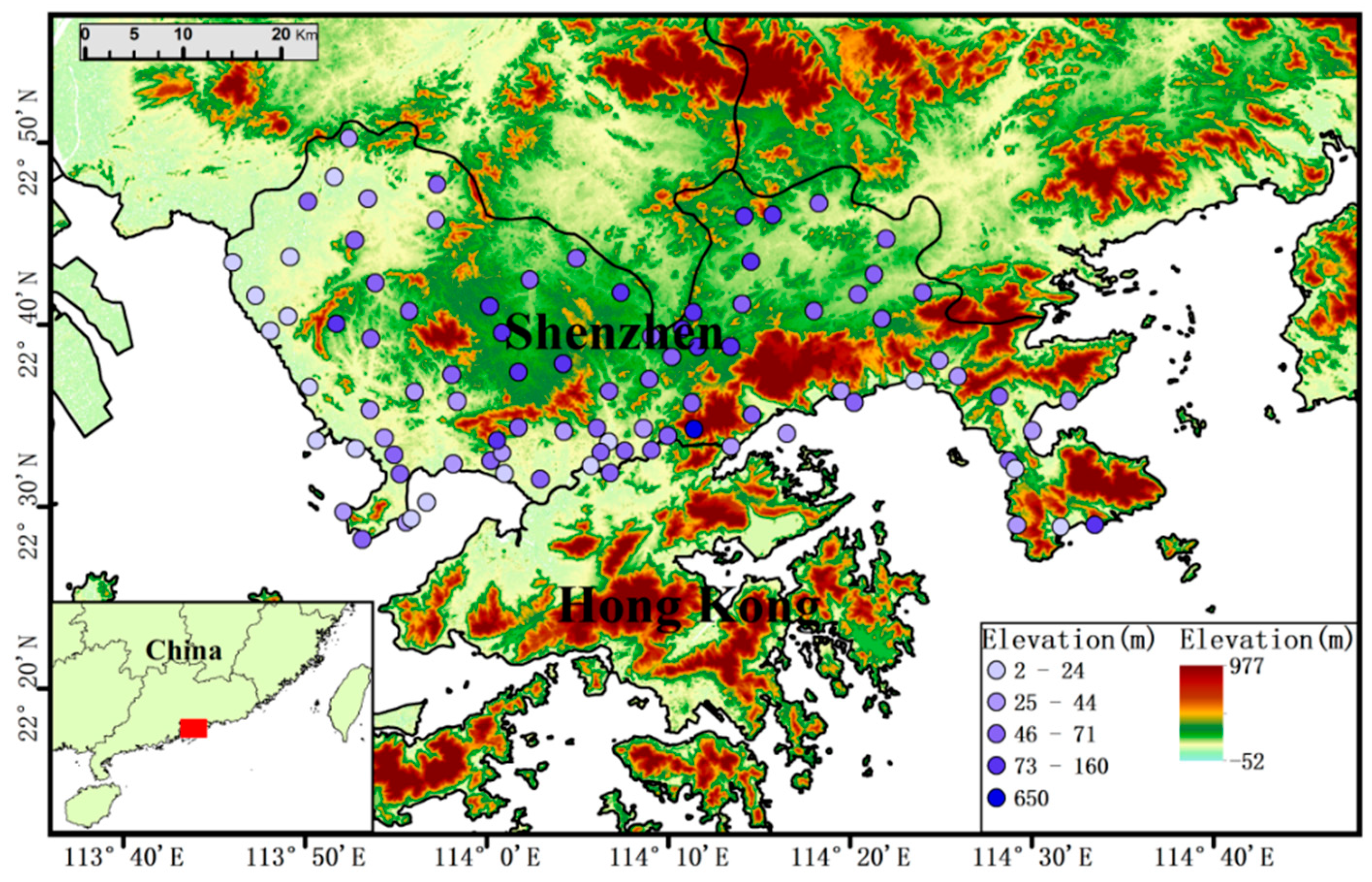
Shenzhen is located on the southern coast of China, covering an area of 1997 km2 between 22°24′–22°52′ N latitude and 113°46′–114°37′ E longitude. Over the past two decades, more than 200 AWSs have been established in Shenzhen. The data used in this study are the hourly wind observations during the 2009–2018 period, which were supplied by Shenzhen Meteorological Bureau (SZMB). The analysis focuses on two types of winds. One is average wind speed (avg-wind), defined as the maximum 10 min average wind speed in an hour; the other one is gust, defined as the maximum 3 s average wind speed in an hour.
Unconditional use of raw data may lead to wrong conclusions; therefore, it is necessary to examine the raw data before proceeding to the analysis. In this study, the data quality control implemented on the AWSs data mainly contains four steps, which basically follow the criteria of some previous studies [37,38]. First, completeness and internal consistency checks were used to exclude the incomplete and erroneous records [37]. A complete record means its information of the wind speed and direction (both for avg-wind and gust) cannot be empty. The rules for the internal inconsistency are identified as (a) the gust speed is less than the avg-wind speed for the same hour and (b) the wind direction is not in the range of [0, 360] (Here the range of [0, 360] refers to a closed interval, meaning that the wind directions are greater or equal to 0 and less or equal to 360, while the range of (0, 360) means that the wind directions are greater than 0 and less than 360). The inconsistent records are considered erroneous and are disregarded in this study. Second, the rule of high/low range limits for wind speed is adopted to exclude the records with extreme high/low values, where the high limits for avg-wind and gust are 45 ms−1 and 100 ms−1, respectively, and the low limits for both are 0 ms−1 [37,38]. Next, a homogeneity check was used to uncover the sudden changes in the mean wind speed by subjective visual inspections [37]. The wind data inhomogeneity caused by AWS relocation or sensor upgrades could result in an unreal trend analysis result. Finally, the qualified AWSs must have records of more than 85% of all hourly observations during the study period.
After the above quality control, wind data from 92 AWSs are qualified for the study period. For the calculations of the average spatial characteristics during the 10-year period, AWSs with 85% of whole data availability are acceptable. The climatological monthly means (CMMs) for all stations can be calculated. For computing the variation trends in wind speed of the AWSs during the study period, the number of hourly records in each month must also have more than 85% availability. Otherwise, the monthly mean in that year must be calculated by the CMM plus the monthly anomaly interpolation. For example, if the hourly wind records for station A in January 2015 are only 60% available, these records are not sufficient to compute the monthly mean wind speed for station A in this month. However, the monthly anomaly (the difference between the CMM and the monthly mean) of station A (AnomV) in January 2015 can be obtained by the spatial anomaly interpolation of the other 91 stations in Shenzhen. Hence, the monthly mean of station A in January 2015 can be computed as the sum of AnomV and CMM.
Figure 1 shows the geographical features of Shenzhen and the distribution of those 92 stations. The average spatial distance between every two stations is less than 5 km. In addition to the observed station data, ERA-Interim data are employed to explore the atmospheric background for the wind conditions in Shenzhen [39].
2.2. Methods
2.2.1. Empirical Orthogonal Function (EOF) Analysis
Due to its simplicity and physical interpretability, the EOF analysis is often used to study possible spatial modes of climate variability and how they change with time [25]. Mathematically, suppose there is a dataset containing wind observations collected from s stations at t discrete time points, and the observed wind data can be represented by the data matrix X (s, t). Then, the anomaly field can be obtained by subtracting the temporal averages at each station. By decomposing the covariance matrix of the anomaly field, the method provides a set of ranked eigenvectors (i.e., EOFs) along with the associated time coefficient. Each EOF explains part of the total variance, and those that explain the largest variances may reflect important physical processes [24,25]. Because the nonuniformly distributed climate data may influence the structure of the computed EOFs, the stations (in Figure 1) data are first interpolated into uniformly distributed gridded data with a resolution of 2 km [24]. The EOF analysis is then implemented to explore the important physical processes based on the gridded monthly mean of the wind data.
2.2.2. Gust Factor
Gust factor (hereafter called GF), as a measure of gustiness, is typically defined as the ratio of the peak wind speed to the sustained wind speed [40]:
In this study, the peak wind speed G refers to the maximum 3 s average gust wind in an hour, and the sustained wind speed U refers to the maximum 10 min average avg-wind in an hour [41]. To better understand the GFs, the values are stratified into three bins based on the avg-wind speeds. This stratification could be useful in forecasting the gust wind. The ranges of avg-wind speed for three GF bins are weak wind bin, less than 5.4 ms−1; medium wind bin, 5.5–13.8 ms−1; and strong wind bin, greater than 13.8 ms−1, which correspond to no more than a force of 3, a force of 4–6, and higher than a force of 6 according to the criterion of the Chinese Meteorological Administration [42].
2.2.3. Trend Analysis
Trends in the annual and seasonal averages of avg-wind were calculated. In addition, the trend of the annual mean wind speed in the troposphere (at 925 hPa and 700 hPa) was also analyzed to explore the possible reasons for the trend of the near-surface wind. Because most of the wind data are nonnormally distributed, nonparametric methods are used in this study. The Sen’s slope estimator was applied to calculate the trend slope [43]. The Mann–Kendall (MK) test was applied to compute the significance levels of the trends [44,45]. A p-value <0.05 is considered that the trend is significant.
2.2.4. Mean Direction
The mean wind direction can reflect the prevailing wind characteristics over a region for a specific season. In this study, Mardia’s method was employed to calculate the mean wind direction [46]. Supposing there is a set of wind directions given by angular measurements , the mean wind direction is computed as follows [46]:
Then, the mean wind direction can be calculated by the solution of the inverse tangent of :
Using the method described above, the monthly mean wind direction was calculated to investigate the variation in wind direction. Furthermore, the wind data were stratified into eight 45° direction bins to assess whether and how the wind direction influences the wind speed patterns.
3. Results and Discussion
3.1. Spatial Wind Characteristics
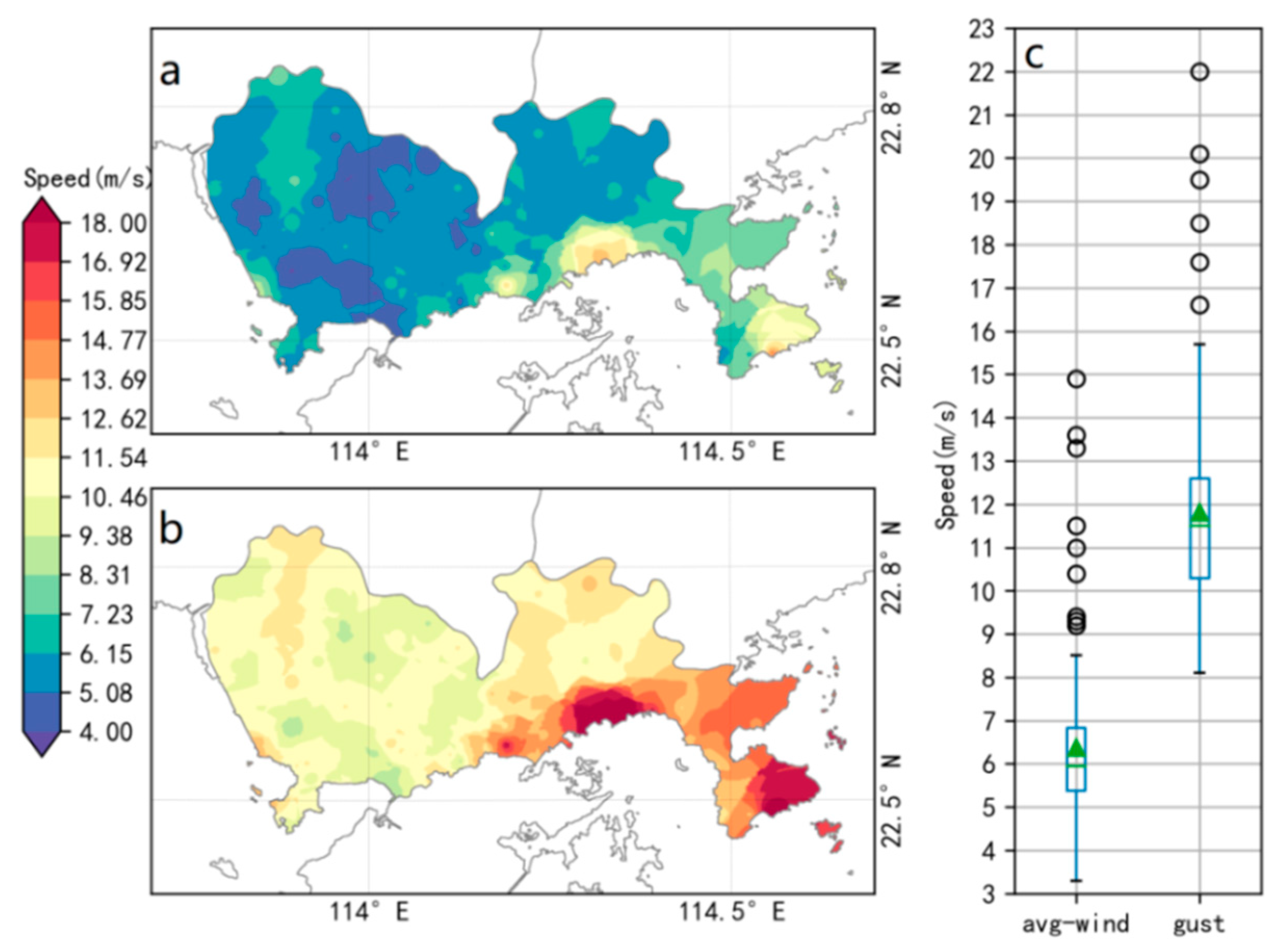
Figure 2 shows the wind distributions of the avg-wind and gust averages in Shenzhen over the 2009–2018 period. Figure 2a,b shows the spatial distributions of the avg-wind and gust, respectively. Figure 2c shows the boxplot of the avg-wind and gust averages at the 92 AWSs in Shenzhen over the 10-year period. The wind distribution patterns are similar in Figure 2a,b. The strongest winds are found along the southeast coast and in the south-central area. Overall, wind is stronger in the east than in the west, and wind is stronger along the coastal areas than in the inland areas. In addition, there are two apparent zones with weak winds in the central west inland areas. From the boxplot (Figure 2c), it can be seen that the median (Q2, the short horizontal line in the middle of the box) and mean (the triangle in the middle of the box) values of avg-wind (10 min average) are approximately 2.5 ms−1. The range of the 25th (Q1) to 75th (Q3) percentiles is [2.2, 2.9]. For the gust (3 s average), the median and mean values are close to 4.5 ms−1, and the corresponding range of the 25th to 75th percentiles is [4.1, 5.1]. Here, the points are drawn as outliers if they are larger than Q3 + 1.5 × (Q3 − Q1) or smaller than Q1 − 1.5 × (Q3 − Q1) for the corresponding avg-wind dataset and gust dataset, respectively.
The result that the average wind along the coastal areas tends to be stronger than that in the inland areas is in accordance with some previous studies [47,48]. A possible explanation for this is that the roughness of the inland surface is much higher than that of the sea water. For coastal cities, such as Shenzhen, the wind would be generally strong over the sea water, followed by the coastal areas and then the inland areas.
In addition to the average wind characteristics, the extreme wind situations in Shenzhen over the 2009–2018 period were investigated. Figure 3 shows the distribution of the 99th percentile of wind at the 92 AWSs over the 10-year period. Figure 3a,b shows the spatial distributions of the 99th percentile of avg-wind and gust, respectively. Figure 3c shows the boxplot of the 99th percentile of the avg-wind and gust at the 92 AWSs over the 10-year period. Comparing the wind situations in Figure 2, the 99th percentile of the avg-wind and gust are more than twice the corresponding average wind speeds. However, there is no significant difference between the distribution patterns of the averages and the 99th percentile, except that the wind speeds are larger in the latter.
3.2. Spatiotemporal Wind Characteristics
3.2.1. Monthly Wind
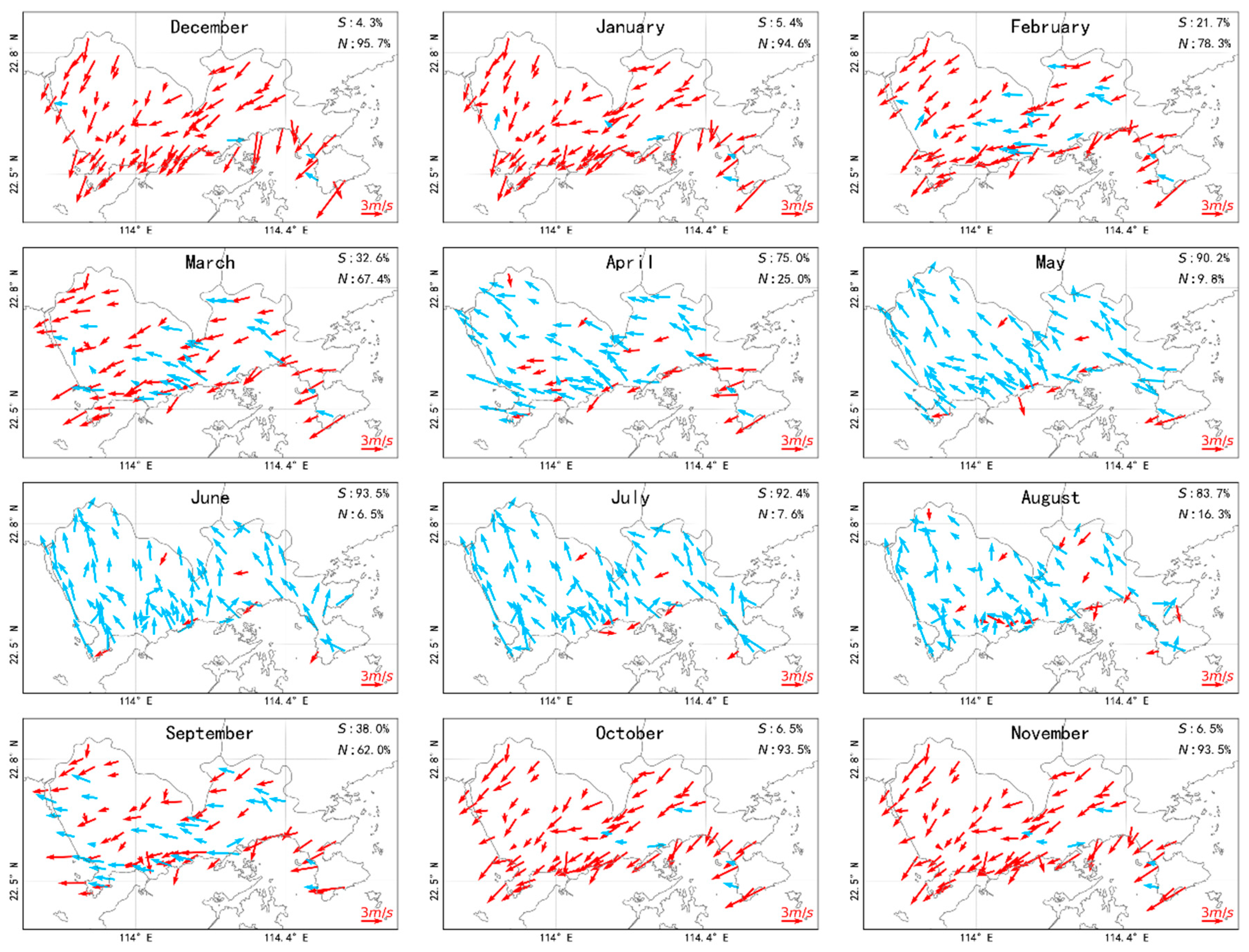
The variations in the 12-month mean wind direction over the 10-year period are shown in Figure 4. As seen from the figure, there is a typical wind direction cycle in Shenzhen. Influenced by the Siberian Anticyclone, the mean wind directions in autumn and winter are mainly northeast and become northernmost around December. More than 95% of the wind directions at the 92 AWSs are northerlies. From January to March, the percentage of the northern wind decreases while the southern wind increases. Summer monsoon is active in spring and summer and has great influence on the prevailing wind in the study area. The wind direction becomes southernmost around July, in which 93.5% of the wind directions at the 92 AWSs are southerlies. According to the percentage of southern and northern winds, two transitions between the winter monsoon and summer monsoon occur around March and September, respectively. These changes in wind directions are consistent with the findings in the neighboring Hong Kong area [49], which shows that the prevailing wind in spring and summer shifts to a southeast direction and gives way to the northeast monsoon in autumn and winter.
Previous studies have found that the origin of the winter monsoon over East Asia can be traced back to the establishment of northwesterly flow via a ridge aloft over Lake Baikal [50]. Then, a large upper-air ridge-trough structure is formed over Siberia to its eastern seaboard and induces southward cold air from the eastern Siberian High [50]. Consequently, the propagation of this cold air brings northeast surface winds in Shenzhen. In contrast, the system of East Asian summer monsoons is more complicated. Zeng et al. [51] found that the summer monsoon before mid-June can be divided into three sub-branches: (a) the Warm Pool region in the West Pacific Ocean and its vicinity, (b) the tropical Indian Ocean region, and (c) the South China Sea region. The three monsoon branches are unified as a whole system after July, which influences the prevailing winds of regions from the Indian Peninsula extending to the South China Sea and 30° N of Eastern China [51]. These tropical monsoons bring Shenzhen south winds associated with warm and humid air. The beginning of the summer monsoon is an important signal of the transition from the dry season to the rainy season [18], and the arrival time and intensity of the summer monsoon directly influences the regional rainfall [18]. Therefore, the study of changes in wind directions could be used in the investigation of the annual variation in local rainfall.
It is worth noting that in Figure 4, there are always some AWSs with different wind directions from the prevailing wind direction in each month. For example, even though the dominant wind direction is northerly in December, some AWSs still have a southerly direction. This wind direction that is different from the prevailing direction is possibly due to the topography alignment [52].
3.2.2. Seasonal Wind
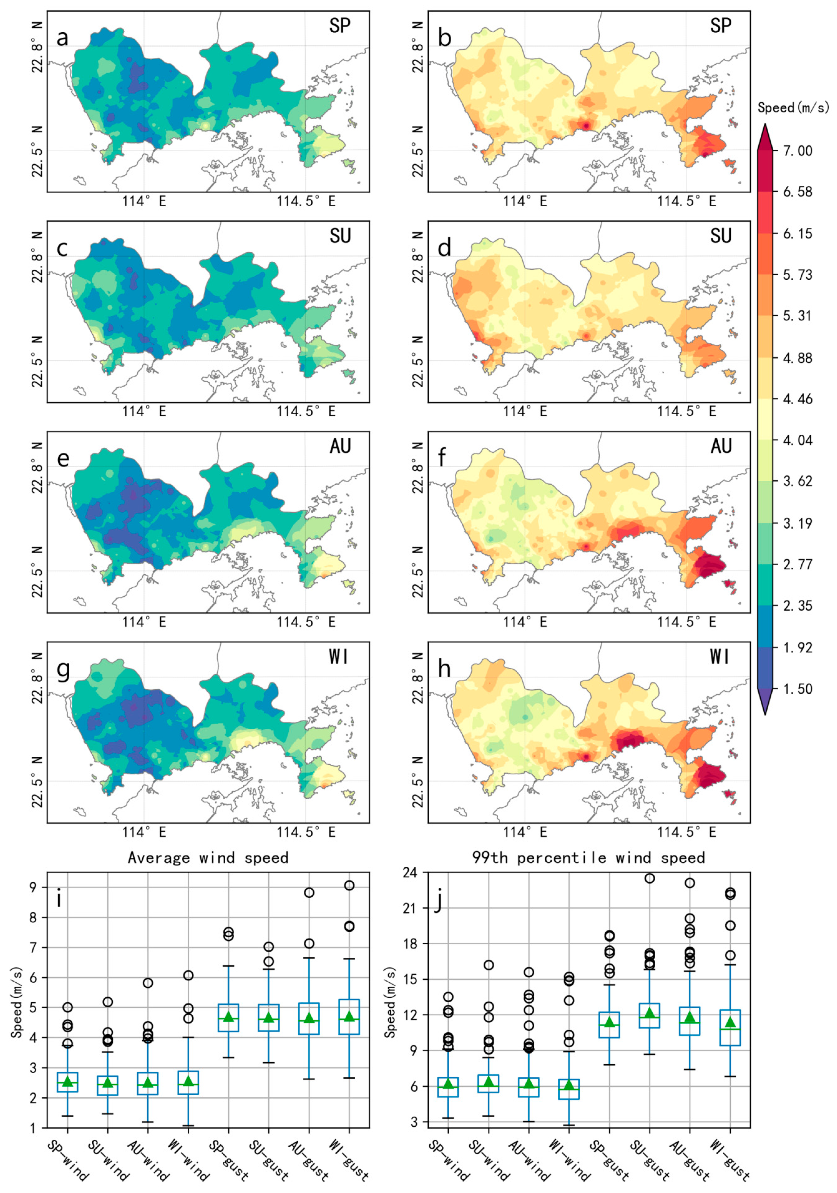
The spatial distributions of the average wind of the avg-wind and gust for the four seasons are illustrated in Figure 5. It can be seen that the average seasonal wind speed distributions can be roughly classified into two types: the autumn–winter type and spring–summer type. In autumn and winter, the strongest winds appear along the southeast coast. The winds in the west, especially in the inland, are significantly less than those in the east. In contrast, the spring–summer type is different from the autumn–winter type. The wind difference between the east area and west area in spring and summer is not as severe as that in autumn and winter. It is worth mentioning that the strongest winds shift to the west coast during the summer time, which is different from the case in the other three seasons. This may be due to the different seasonal prevailing wind directions, which are shown in Figure 4. In summer, the prevailing wind direction is southerly. During this season, the South China Sea summer monsoon and Southwest monsoon occur frequently [51]. This should be the reason why the west coast of Shenzhen also suffers from a strong wind influence in summer.
Furthermore, the seasonal mean of avg-wind speeds and 99th percentile of the seasonal avg-wind speeds at those 92 AWSs were analyzed (Figure 5i,j and Table 1 and Table 2). According to Figure 5i and Table 1, the average wind speeds tend to be greater in spring and winter (relatively greater mean and median), which is consistent with the study on wind speed in China [19]. The study by Lau and Lau indicated that high-frequency midlatitude disturbances caused frequent cold surges, thus strengthening the surface winds in East Asia [53]. Therefore, the greater wind speeds of the winter monsoon are attributed to the frequent cold surges. However, the situations are different for the 99th percentile wind speeds (Figure 5j and Table 2) in terms of the mean and median. Wind speed is largest in summer, followed by autumn, winter, and spring. It is worth noting that the strong winds in winter and spring are mainly caused by the Siberian Anticyclone [54], while in summer and autumn, the strong winds are mainly due to the frequent tropical cyclones [55]. The difference here suggests that the winter monsoon may bring higher continuous wind power, while the extreme windy weather caused by the monsoon is less destructive than the winds caused by tropical cyclones.
From Figure 4 and Figure 5, it can be seen that the wind direction transition time is close to the time of the seasonal wind speed pattern change. Then, it is inferred that the seasonal wind direction may have a great influence on the wind spatial distribution. Therefore, the relationship between the wind direction and the wind speed distribution is further investigated.
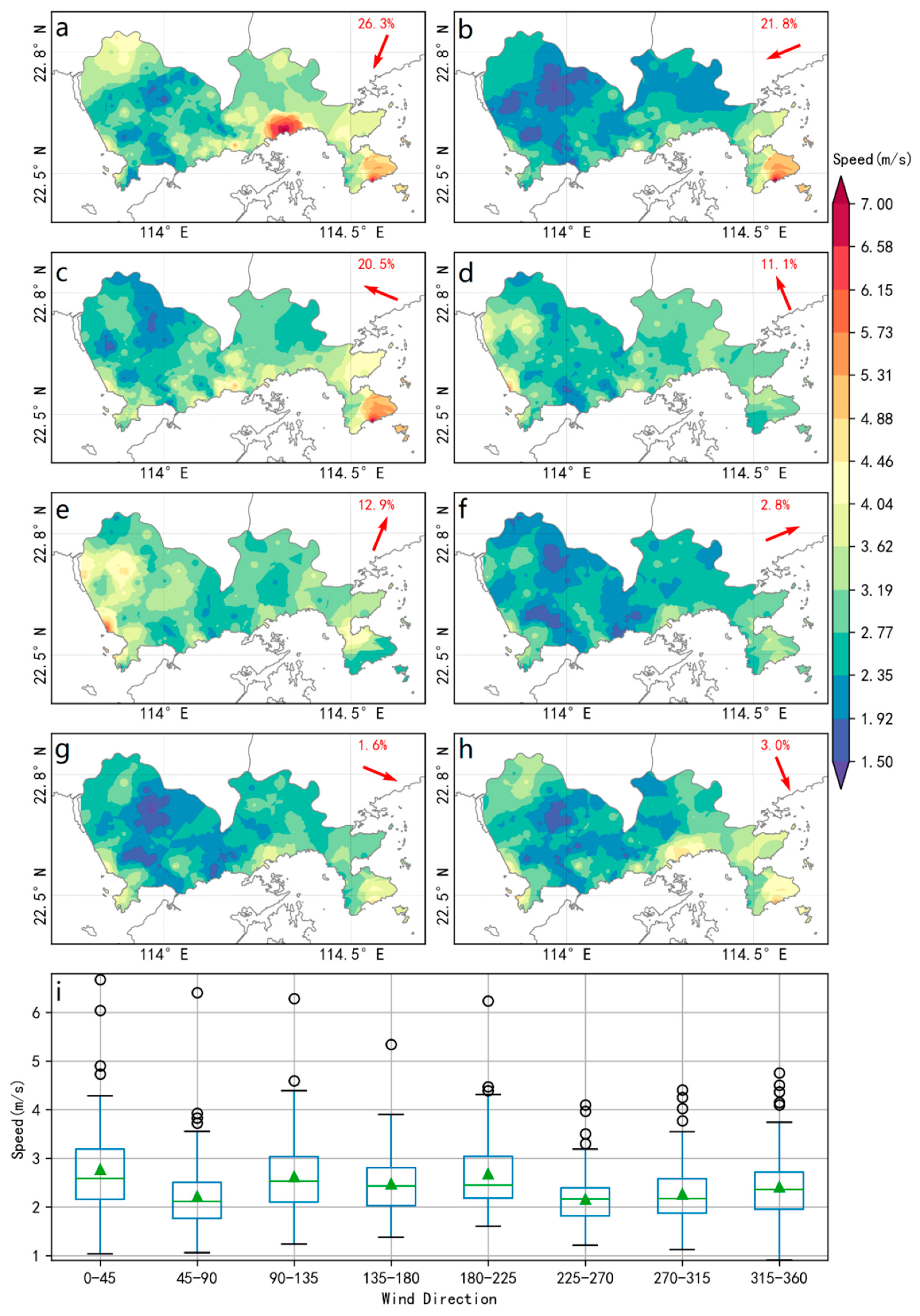
Based on the hourly mean wind direction, the avg-wind speeds are stratified into eight direction bins, which are [0°, 45°), [45°, 90°), [90°, 135°), …, and [315°, 360°). The spatial avg-wind distributions in Shenzhen under the eight wind directions are shown in Figure 6. The percentage of each of the wind directions during the 10-year period was also computed and is shown on the top right of each subplot. As seen in Figure 6, the most prevailing wind direction in Shenzhen is the 0–45° wind (Figure 6a), accounting for 26.3% of the total wind directions. The second and third prevailing wind directions are 45–90° (Figure 6b) and 90–135° (Figure 6c), respectively. The southwest wind direction of 180–225° (Figure 6e) ranks fourth. Figure 6i shows the boxplot of the mean avg-wind at the 92 AWSs during the past 10-year period under the eight different wind directions. Figure 6 shows that for the avg-wind, the strongest wind direction is 0–45°, followed by 90–135° and 180–225°. Under the wind directions of 0–45° and 90–135°, strong avg-wind occurs along the southeast coast, while under the wind direction of 180–225°, the avg-wind is stronger along the west coast than along the southeast coast.
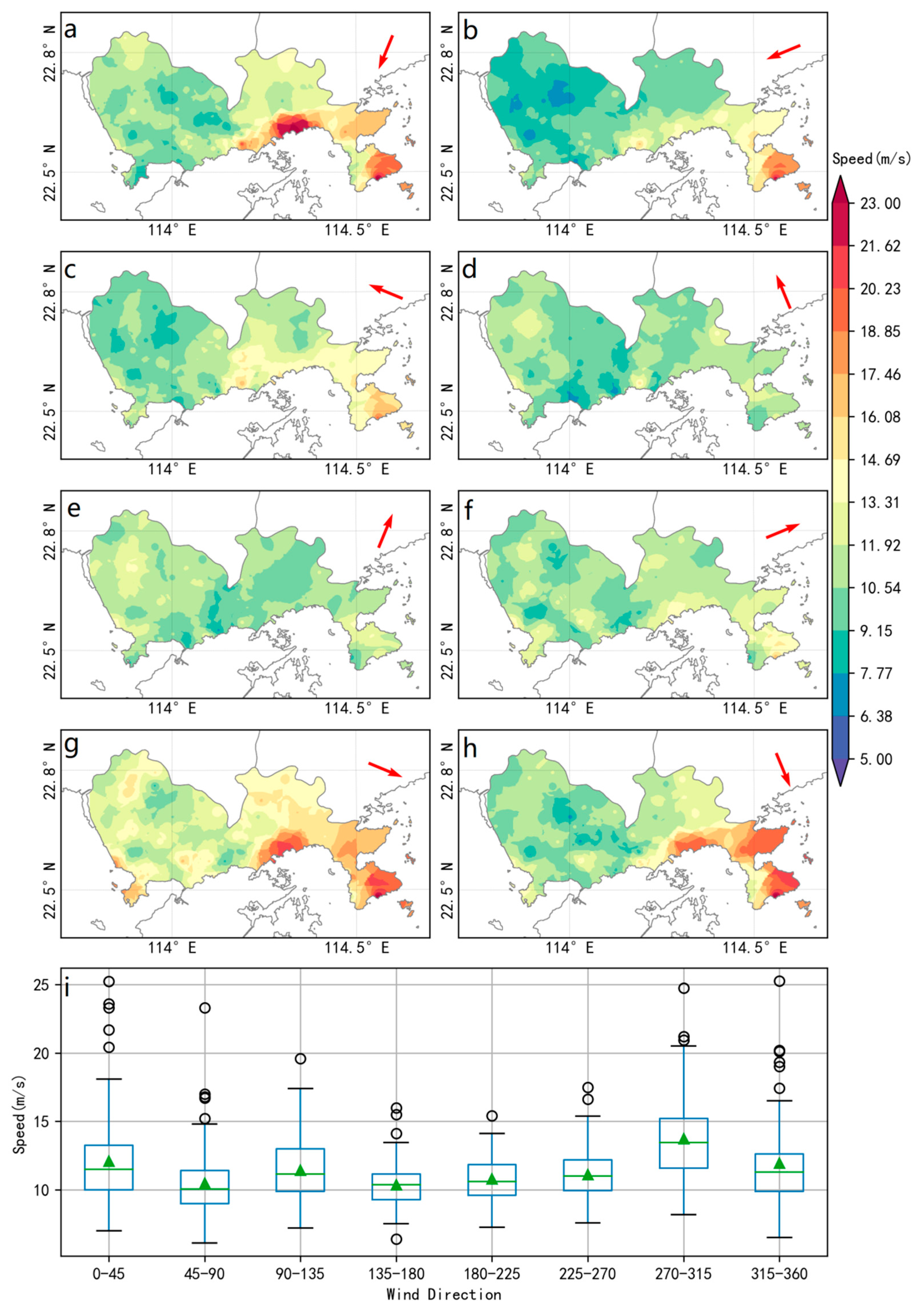
As gust wind is more destructive than avg-wind [56], the extreme situation of the 99th percentile of the gust wind at the 92 AWSs under the eight different wind directions during the past 10-year period was also explored. Figure 7 shows the spatial distributions of the 99th percentile of the gust wind in Shenzhen under the eight wind directions.
As seen from Figure 7i, there are many gust wind outliers at the 92 AWSs for the 0–45° wind direction, and these outliers are more than 20 ms−1. The 0–45° wind direction is the typical direction across the Shenzhen area when there is a tropical cyclone over the South China Sea in the southwest direction relative to Shenzhen. In the 0–45° direction, severe gust winds mainly occur along the southeast coast (Figure 7a). The second and third worst cases are the 270–315° and 315–360° wind directions, respectively. These are the two typical wind directions in Shenzhen when experiencing cold fronts in winter and spring. Figure 7g,h shows that the southeast coast suffers the most. When the dominant wind direction is 270–315°, the entire Shenzhen region experiences strong gust winds, including the west coast and inland areas (see Figure 7g,i).
As seen from Figure 4, Figure 5, Figure 6 and Figure 7, the wind direction has an obvious influence on the spatial distribution of wind speed. This finding is consistent with some previous studies that suggest a strong coherence between the wind speed distribution and wind direction [20,57]. These findings may be helpful to the local government and authorities in decision making for wind disaster prevention and mitigation.
3.2.3. Trend Analysis
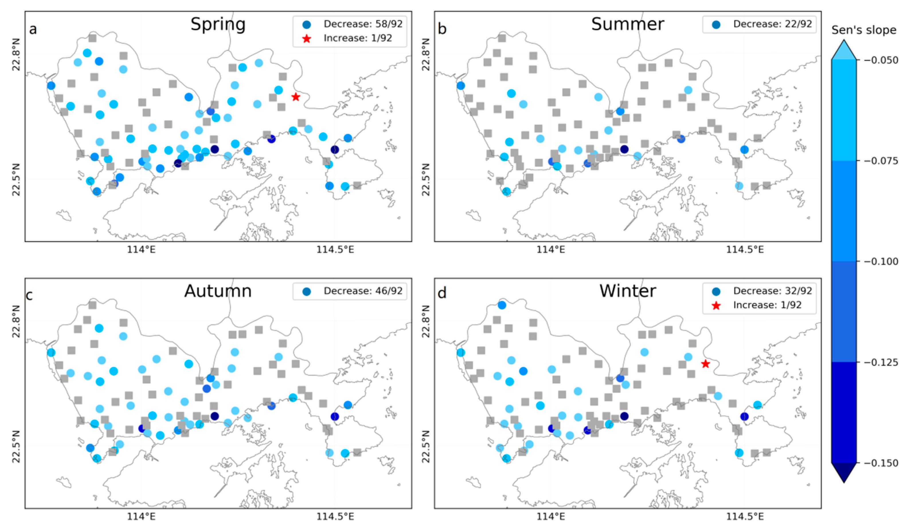
The trends of the yearly and seasonal mean of the avg-wind speeds and gust wind speeds at each AWS were analyzed by the Sen’s slope method and the Mann–Kendall test (Table 3). As seen in Table 3, the wind speed in Shenzhen is mainly decreasing. More than 90% of AWSs have decreasing trends in the annual mean of avg-wind and gust wind. Approximately 70% of these decreasing trends are statistically significant. Seasonally, the trends are different from each other. The wind decrease in spring is relatively severe, followed by autumn. In spring and autumn, 95% (98%) and 89% (91%) of the stations have decreasing trends in avg-wind (gust wind). The percentages of the significant decreasing trends in avg-wind (gust wind) for spring and autumn are 63% (64%) and 50% (47%), respectively. In summer and winter, more than 75% of AWSs also have decreasing trends, but the percentage of stations with significant decreasing trends in wind speed is much less than that in spring and autumn. It is worth noting that there is only one AWS with a significant increasing trend in avg-wind in spring and winter.
Figure 8 shows the spatial distribution of the seasonal trend of the avg-wind at the 92 AWSs. The stations with significant decreasing trends are denoted by blue dots, while the station with a significant increasing trend is denoted by a red star. Otherwise, the stations with insignificant trends are in gray. The distribution of the AWSs with significant trends is relatively uniform. Figure 8 shows that the Sen’s slopes of avg-wind trends at most of the AWSs range from −0.1 ms−1/year to 0 ms−1/year with a mean value of approximately −0.06 ms−1/year.
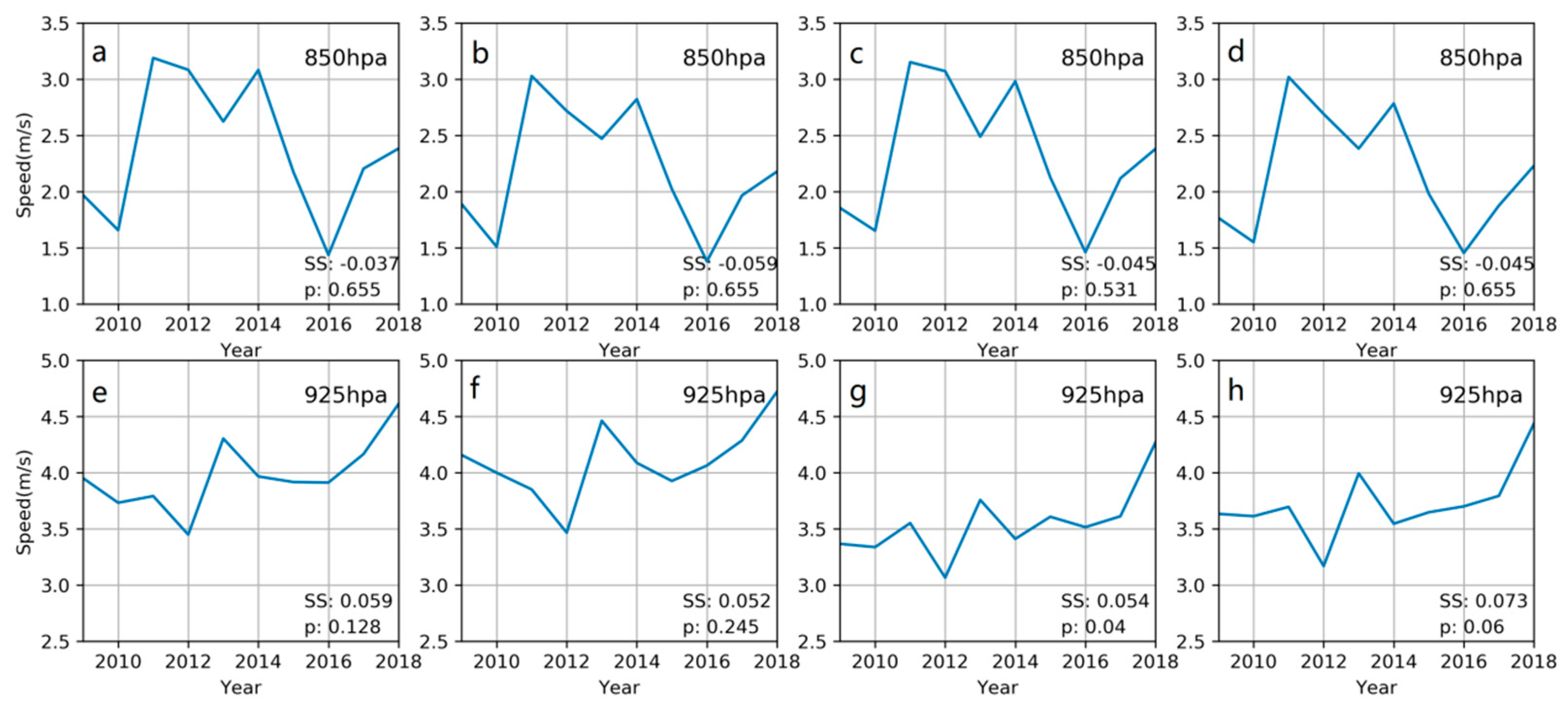
The above results show that the wind is decreasing at most of the AWSs in Shenzhen. This finding is consistent with the conclusion that there has been a decreasing trend in the mean wind speed in China for the past few decades [17,22]. Some previous studies have suggested that under the background of climate change, the lower-tropospheric wind is weakening [17,22]. This may be the reason for the universal mean wind speed decrease in China. To determine why wind speeds are declining in the study area, the ERA-Interim reanalysis data from 2009 to 2018 were analyzed. For ERA-Interim reanalysis data with a spatial resolution of approximately 80 km, four points that cover or are close to the Shenzhen area were chosen to explore the tropospheric variation during the study period. The four points are (113.906° E, 22.105° N), (113.906° E, 22.807° N), (114.609° E, 22.105° N), and (114.609° E, 22.807° N). Figure 9 shows the wind variations in these four points at 925 hPa and 850 hPa. As seen from the figure, no point shows a significant decreasing trend in the annual mean wind speeds at 925 hPa and 850 hPa over the study area. Over the past several decades, Shenzhen has experienced rapid development and large changes in land use and land cover [58,59]. This rapid urbanization development in Shenzhen has led to an increase in the surface roughness of the city and therefore resulted in a decrease of the mean wind in the area [60].
3.3. Gust Factor
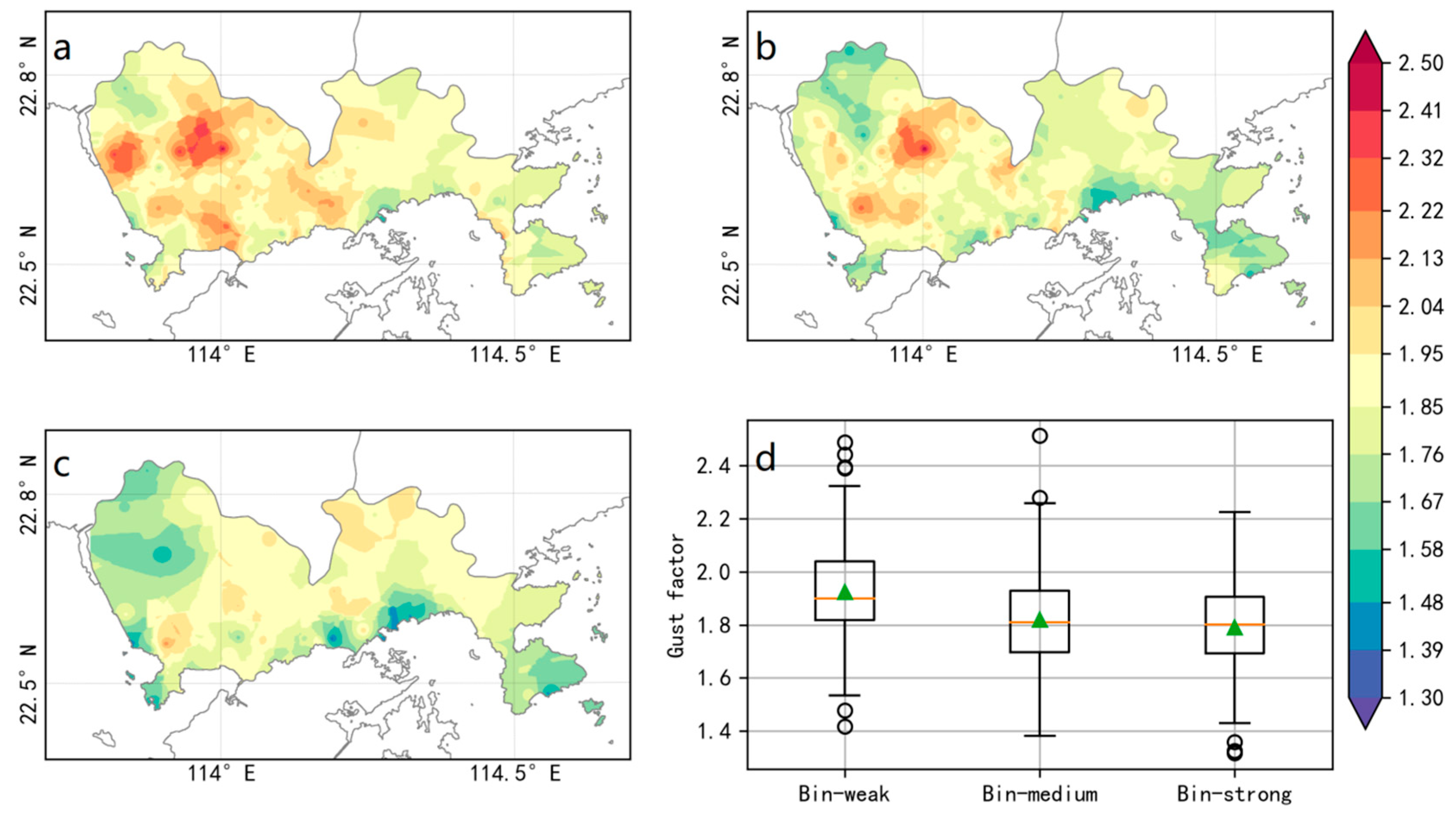
Gust factor (GF) is a measure of gustiness and is sensitive to the mean wind speed. According to the method mentioned in Section 2.2.2, the GFs of the 92 AWSs are stratified into three bins according to the wind force of their mean wind (i.e., avg-wind). Figure 10 shows the distributions of the average GFs for the three bins. The data sizes of these bins account for 95.42%, 4.53%, and 0.05% of the total data, respectively. As 13.8 ms−1 is a relatively high speed for avg-wind, only 70 AWSs appear in the strong wind bin. Figure 10a–c shows similar spatial distributions. The GFs in the coastal areas are generally lower than those in the inland areas. On the other hand, there are also some discrepancies in Figure 10a–c. For example, the GFs in northwestern Shenzhen and the central west inland are high in Figure 10a; however, GFs in northwestern Shenzhen are low in Figure 10c. As seen in Figure 2a, northwestern Shenzhen is the area with the lowest avg-wind. Since the strong wind bin only includes the data samples larger than 13.8 ms−1, there should be very few data in northwestern Shenzhen in Figure 9c. This is why GF patterns in northwestern Shenzhen are different in Figure 10a–c. Generally, the maximum GFs appear in the central west inland, most of which are between 1.8 and 2.3. In contrast, the range of most GFs in the northeast inland is [1.7, 2.0], while the range of GFs along the coastal area is [1.4, 1.8]. The distribution pattern of GFs in Figure 10 seems to be the opposite of the distribution of yearly average wind speed, as presented in Figure 2.
3.4. Spatial Wind Characteristics
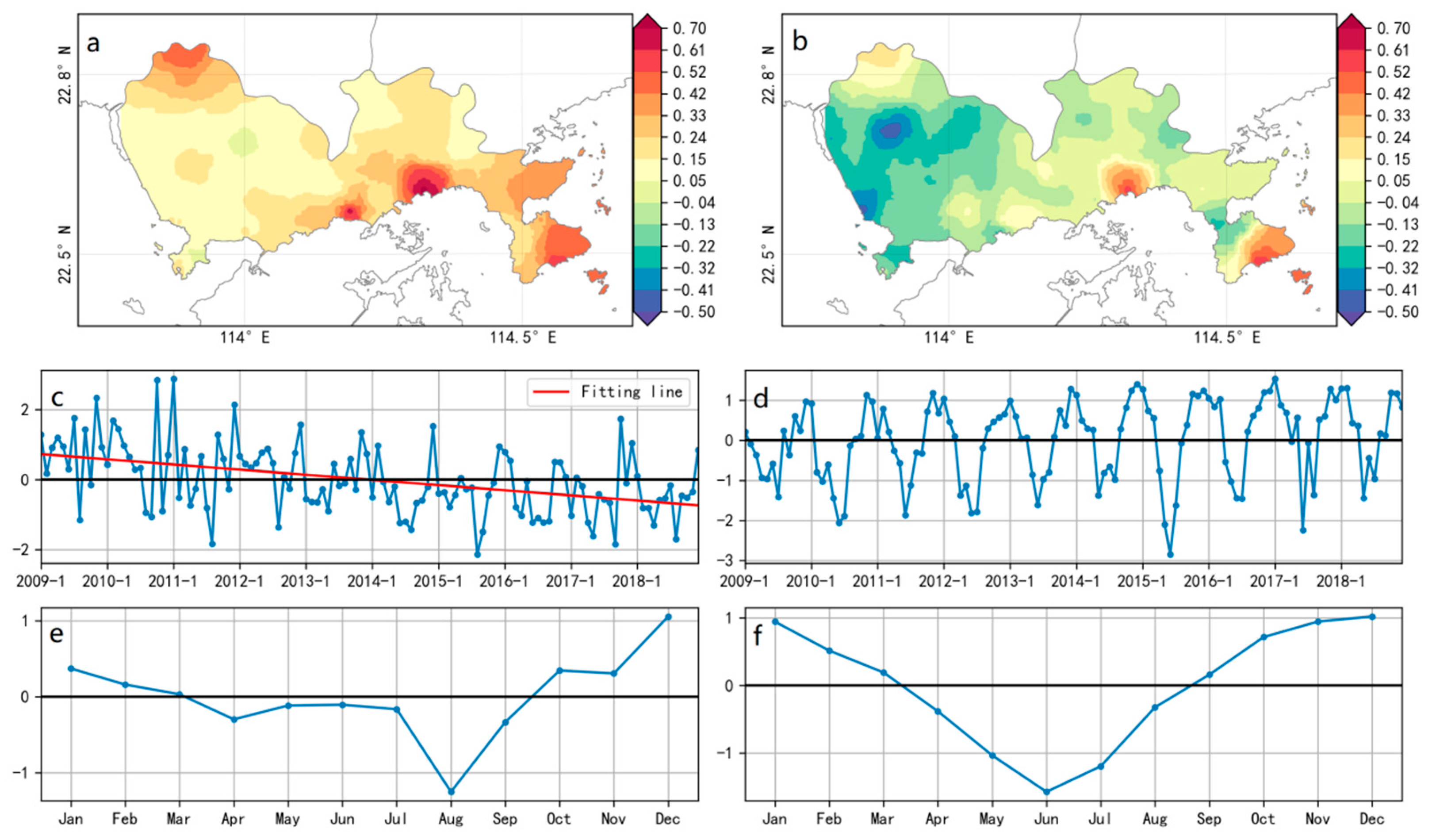
The monthly means of the avg-wind data of the AWSs from 2009 to 2018 in Shenzhen were first interpolated into gridded data and then analyzed by the EOF method. The leading two EOF modes can explain most of the total variance of the monthly mean of the avg-wind speed. The first EOF mode (Figure 11a) explains 48% of the total variance. High values of the spatial pattern appear along the southeast coast, northwest corner, and central-south mountain area, which are similar to the pattern of the annual mean of avg-wind. In addition, nearly all the values are positive, thereby indicating that all the AWSs have synchronized wind speed changes in this pattern. In terms of the corresponding time coefficients (Figure 11c), there exists a significant decreasing (p < 0.05) trend. These results suggest that the avg-wind speeds are decreasing in the whole area, which is in accordance with the results of the trend analysis.
The second EOF mode (Figure 11b) explains 28% of the total variance. The values in the central-southern mountain area and in the southeastern and northwestern corners are positive. In contrast, most of the values in western Shenzhen are negative. The time coefficients for the second EOF mode, presented in Figure 11d, show a distinct annual cyclical change. Figure 11f shows that the coefficients are positive in autumn and winter and negative in spring and summer. Therefore, the results of the second EOF mode indicate that the avg-wind tends to be greater in the western area in spring and summer and the opposite in autumn and winter.
4. Conclusions
This study examines the spatiotemporal characteristics of the near-surface wind by using high spatial resolution data over Shenzhen from 2009 to 2018. The results show that the large-scale atmospheric circulation, local topographic factors, and human activities have combined to shape the intricate patterns of the near-surface winds in Shenzhen.
Wind is stronger along the coastal area than inland, and wind is generally stronger in eastern Shenzhen than in western Shenzhen. The GF tends to decline with increasing wind speed, and the spatial distribution of GFs is almost the opposite of the wind speed distribution. The GFs along the coastal area are concentrated in [1.4, 1.8], while the GFs in the central-western inland area are between 1.8 and 2.3, and the GFs in the northeastern inland area are concentrated in [1.7, 2.0].
Dominated by the large-scale atmospheric circulation, the near-surface wind field in Shenzhen has significant seasonal variation characteristics, which can be classified into two patterns, spring–summer type and autumn–winter type. The transitions between the two patterns occur in approximately March and September. In spring and summer, the prevailing wind directions are mainly southerlies, while the prevailing wind directions are northerlies in autumn and winter.
The annual and seasonal mean wind speeds tend to decrease at most of the stations in Shenzhen, especially the spring wind. During the past ten years, the annual mean surface avg-wind speed has decreased by approximately 0.4 ms−1. Since there is no significant downward trend in the wind speed of the troposphere aloft over Shenzhen, the decrease in the surface wind is mainly due to the urbanization development.
Author Contributions
Conceptualization, C.L. and Q.L.; methodology, C.L., Q.L. and Y.W.; software, C.L., X.L. and Q.L.; validation, C.L., Q.L. and X.L.; formal analysis, C.L., Q.L., W.Z.; investigation, C.L. and Q.L.; resources, Q.L., H.Z., and X.W.; data curation, C.L., and X.L.; writing—original draft preparation, C.L.; writing—review and editing, Q.L., W.Z., R.A., Y.W. and D.H.; visualization, C.L.; supervision, Q.L.; project administration, Q.L.; and funding acquisition, Q.L. All authors have read and agreed to the published version of the manuscript.
Funding
This study was supported by the Science and Technology Department of Guangdong Province with Grant of 2019B111101002 and the Innovation of Science and Technology Commission of Shenzhen Municipality Ministry with Grants of JCYJ20170413164957461 and GGFW2017073114031767.
Conflicts of Interest
The authors declare that they have no conflicts of interest.
References
- Paul, V.; Tonts, M. Containing Urban Sprawl: Trends in Land Use and Spatial Planning in the Metropolitan Region of Barcelona. J. Environ. Plan. Manag. 2005, 48, 7–35. [Google Scholar] [CrossRef]
- Boyle, R.; Mohamed, R. State Growth Management, Smart Growth and Urban Containment: A Review of the US and a Study of the Heartland. J. Environ. Plan. Manag. 2007, 50, 677–697. [Google Scholar] [CrossRef]
- Tian, L.; Li, Y.; Yan, Y.; Wang, B. Measuring Urban Sprawl and Exploring the Role Planning Plays: A Shanghai case study. Land Use Policy 2017, 67, 426–435. [Google Scholar] [CrossRef]
- Schell, L.M.; Ulijaszek, S.J. Urbanism, Health and Human Biology in Industrialized Countries; Cambridge University Press: London, UK, 1999; pp. 59–60. ISBN 978-0511525698. [Google Scholar]
- Yang, P.; Ren, G.; Liu, W. Spatial and temporal characteristics of Beijing urban heat island intensity. J. Appl. Meteorol. Climatol. 2013, 52, 1803–1816. [Google Scholar] [CrossRef]
- Zhang, C. Urban climate and air pollution in Shanghai. Energy Build. 1991, 16, 647–656. [Google Scholar] [CrossRef]
- Savard, J.-P.L.; Clergeau, P.; Mennechez, G. Biodiversity concepts and urban ecosystem. Landscape Urban Plan. 2000, 48, 131–142. [Google Scholar] [CrossRef]
- Zhang, L.; Li, Q.; Guo, Y.; Yang, Z.; Zhang, L. An investigation of wind direction and speed in a featured wind farm using joint probability distribution methods. Sustainability 2018, 10, 4338. [Google Scholar] [CrossRef] [Green Version]
- Wang, F.; Duan, K.; Zou, L. Urbanization Effects on Human-Perceived Temperature Changes in the North China Plain. Sustainability 2019, 11, 3413. [Google Scholar] [CrossRef] [Green Version]
- Jung, C.; Schindler, D. Modelling monthly near-surface maximum daily gust speed distributions in southwest Germany. Int. J. Climatol. 2016, 36, 4058–4070. [Google Scholar] [CrossRef]
- Klawa, M.; Ulbrich, U. A model for the estimation of storm losses and the identification of severe winter storms in Germany. Nat. Hazard Earth Syst. Sci. 2003, 3, 725–732. [Google Scholar] [CrossRef] [Green Version]
- Manasseh, R.; Middleton, H.M. The surface wind gust regime and aircraft operations at Sydney Airport. J. Wind Energy Ind. Aerodyn. 1999, 79, 269–288. [Google Scholar] [CrossRef]
- Schindler, D.; Grebhan, K.; Albrecht, A.; Schönborn, J.; Kohnle, U. GIS-based estimation of the winter storm damage probability in forests: A case study from Baden-wuerttemberg (southwest Germany). Int. J. Biometeorol. 2012, 56, 57–69. [Google Scholar] [CrossRef]
- Berkowicz, R.; Palmgren, F.; Hertel, O.; Vignati, E. Using measurements of air pollution in streets for evaluation of urban air quality—Meterological analysis and model calculations. Sci. Total Environ. 1996, 189–190, 259–265. [Google Scholar] [CrossRef]
- Wang, T.; Xue, L.; Brimblecombe, P.; Lam, Y.F.; Li, L.; Zhang, L. Ozone pollution in China: A review of concentrations, meteorological influences, chemical precursors, and effects. Sci. Total Environ. 2017, 575, 1582–1596. [Google Scholar] [CrossRef] [PubMed]
- Wu, J.; Zha, J.; Zhao, D. Estimating the impact of the changes in land use and cover on the surface wind speed over the East China Plain during the period 1980–2011. Clim. Dyn. 2016, 46, 847–863. [Google Scholar] [CrossRef]
- Guo, H.; Xu, M.; Hu, Q. Changes in near-surface wind speed in China: 1969–2005. Int. J. Climatol. 2011, 31, 349–358. [Google Scholar] [CrossRef]
- Ding, Y.; Li, C.; Liu, Y. Overview of the South China Sea monsoon experiment. Adv. Atmos. Sci. 2004, 21, 343–360. [Google Scholar] [CrossRef]
- Liu, F.; Sun, F.; Liu, W.; Wang, T.; Wang, H.; Wang, X.; Lim, W.H. On wind speed pattern and energy potential in China. Appl. Energy 2019, 236, 867–876. [Google Scholar] [CrossRef]
- Klink, K. Complementary use of scalar, directional, and vector statistics with an application to surface winds. Prof. Geogr. 1998, 50, 3–13. [Google Scholar] [CrossRef]
- Azorin-Molina, C.; Vicente-Serrano, S.M.; McVicar, T.R.; Jerez, S.; Sanchez-Lorenzo, A.; Lopez-Moreno, J.; Revuelto, J.; Trigo, R.M.; Lopez-Bustins, J.; Espirito-Santo, F. Homogenization and assessment of observed near-surface wind speed trends over Spain and Portugal, 1961–2011. J. Clim. 2014, 27, 3692–3712. [Google Scholar] [CrossRef]
- Jiang, Y.; Luo, Y.; Zhao, Z.; Tao, S. Changes in wind speed over China during 1956–2004. Theor. Appl. Climatol. 2014, 99, 421–430. [Google Scholar] [CrossRef]
- Mcvicar, T.R.; Roderick, M.L.; Donohue, R.J.; Li, L.T.; Niel, T.G.V.; Thomas, A.; Grieser, J.; Jhajharia, D.; Himri, Y.; Mahowald, N.M.; et al. Global review and synthesis of trends in observed terrestrial near-surface wind speeds: Implications for evaporation. J. Hydrol. 2012, 416–417, 182–205. [Google Scholar] [CrossRef]
- Hannachi, A. A Primer for EOF Analysis of Climate Data; Department of Meteorology, University of Reading: Reading, UK, 2004; 33p, Available online: http://www.o3d.org/eas-6490/lectures/EOFs/eofprimer.pdf (accessed on 21 October 2019).
- Lorenz, E.N. Empirical Orthogonal Functions and Statistical Weather Prediction; Scientific Report No. 1; Massachusetts Institute of Technology Department of Meteorology: Cambridge, MA, USA, 1956; Available online: http://bobweigel.net/csi763/images/pdf/Lorenz1956.pdf (accessed on 21 October 2019).
- Ludwig, F.L.; Horel, J.; Whiteman, C.D. Using EOF Analysis to Identify Important Surface Wind Patterns in Mountain Valleys. J. Appl. Meteorol. 2004, 43, 969–983. [Google Scholar] [CrossRef] [Green Version]
- Hughes, M.; Hall, A.; Fovell, R.G. Dynamical controls on the diurnal cycle of temperaturein complex topography. Clim. Dyn. 2007, 29, 277–292. [Google Scholar] [CrossRef]
- Beaver, S.; Palazoglu, A. Cluster Analysis of Hourly Wind Measurements to Reveal Synoptic Regimes Affecting Air Quality. J. Appl. Meteorol. Climatol. 2006, 45, 1710–1726. [Google Scholar] [CrossRef]
- Hannachi, A.; Jolliffe, I.T.; Stephenson, D.B. Empirical Orthogonal Functions and Related Techniques in Atmospheric Science: A review. Int. J. Climatol. 2007, 27, 1119–1152. [Google Scholar] [CrossRef]
- Huang, D. Analysis and forecast of cold wave in Guangdong. J. Guangdong Meteorol. 1995, 4, 2–6. (In Chinese) [Google Scholar]
- Lin, A.; Wu, S. The Characteristics of Cold Wave Action in Guangdong Province During Recent 44 Years. J. Trop. Meteorol. 1998, 14, 337–343. (In Chinese) [Google Scholar] [CrossRef]
- Tang, X.; Liu, H.; Pan, A.; Liang, B.; Li, Y.; Wang, T. Analysis of disastrous features of landing typhoon in coastal regions of Guangdong province in recent 50 years. Sci. Geogr. Sin. 2003, 23, 182–187. (In Chinese) [Google Scholar] [CrossRef]
- Zhang, T.; Fang, C.; Zhu, W.; Zhang, G.; Zhou, Q. Analysis of the 17 April 2011 severe convective weather in Guangdong. Meteorol. Mon. 2012, 38, 814–818. (In Chinese) [Google Scholar]
- Zhang, E.J.; Zhang, J.J.; Zhao, X.Y.; Zhang, X.L. Study on urban heat island effect in Shenzhen. J. Nat. Disaster 2008, 17, 19–24. (In Chinese) [Google Scholar] [CrossRef]
- Liu, X.Z.; Heilig, G.K.; Chen, J.; Heino, M. Interactions between Economic Growth and Environmental Quality in Shenzhen, China’s First Special Economic Zone. Ecol. Econ. 2007, 62, 559–570. [Google Scholar] [CrossRef] [Green Version]
- Wei, X.; Wang, D.; He, J.; Cheng, Z. Characteristics analysis on gust factors over coastal areas in Shenzhen. Guangdong Meteorol. 2016, 38, 33–36. (In Chinese) [Google Scholar] [CrossRef]
- Feng, S.; Hu, Q.; Qian, W. Quality control of daily meteorological data in China, 1951-2000: A new dataset. Int. J. Climatol. 2004, 24, 853–870. [Google Scholar] [CrossRef]
- Meek, D.W.; Hatfield, J.L. Data quality checking for single station meteorological databases. Agric. For. Meteorol. 1994, 69, 85–109. [Google Scholar] [CrossRef]
- European Centre for Medium-Range Weather Forecasts, 2012: ERA-Interim Project, Monthly Means. Research Data Archive at the National Center for Atmospheric Research, Computational and Information Systems Laboratory. Available online: https://rda.ucar.edu/datasets/ds627.1/ (accessed on 11 October 2019).
- Tyner, B.; Aiyyer, A.; Blaes, J.; Hawkins, D.R. An examination of wind decay, sustained wind speed forecasts, and gust factors for recent tropical cyclones in the Mid-Atlantic region of the United States. Weather Forecast. 2015, 30, 153–176. [Google Scholar] [CrossRef]
- Liu, B.; Li, Q.; Yang, L.; Li, H.; Cao, Y.; Tang, X.; Sun, S.; Sun, L. Seasonal wind characteristics in Shenzhen area. Meteorol. Mon. 2019, 45, 263–273. (In Chinese) [Google Scholar]
- China Meteorological Administration. The Criterion of Wind Scale in China. Available online: http://www.cma.gov.cn/2011xzt/20120816/2012081601/201208160101/201407/t20140717_252607.html (accessed on 21 October 2019). (In Chinese)
- Sen, P.K. Estimates of the regression coefficient based on Kendall’s tau. J. Am. Stat. Assoc. 1968, 63, 1379–1389. [Google Scholar] [CrossRef]
- Mann, H.B. Nonparametric tests against trend. Econometrica 1945, 13, 245–259. [Google Scholar] [CrossRef]
- Kendall, M.G. Rank Correlation Methods, 4th ed.; Charles Griffin: London, UK, 1970. [Google Scholar]
- Mardia, K.V.; Jupp, P.E. Directional Statistics, 1st ed.; John Wiley & Sons, Inc.: New York, NY, USA, 2000; pp. 15–17. ISBN 0-471-95333-4. [Google Scholar]
- Achberger, C.; Chen, D.; Alexandersson, H. The surface winds of Sweden during 1999–2000. Int. J. Climatol. 2006, 26, 159–178. [Google Scholar] [CrossRef]
- Xue, H.; Zhu, R.; Yang, Z. Study on land wind speed variation in coastal area. Acta Energ. Sol. Sin. 2002, 23, 207–210. (In Chinese) [Google Scholar]
- Yan, Y.Y. Surface wind characteristics and variability in Hong Kong. Weather 2007, 62, 312–316. [Google Scholar] [CrossRef]
- Chen, T.C.; Yen, M.C.; Huang, W.R.; Gallus, W.A. An East Asian Cold Surge: Case Study. Mon. Weather Rev. 2002, 130, 2271–2290. [Google Scholar] [CrossRef]
- Zeng, Q.; Zhang, D.; Zhang, M.; Zuo, R.; He, J. The abrupt seasonal transitions in the atmospheric general circulation and the onset of monsoons part I: Basic theoretical method and its application to the analysis of climatological mean observations. Climatic Environ. Res. 2005, 10, 285–302. (In Chinese) [Google Scholar]
- Martner, B.E.; Marwitz, J.D. Wind characteristics in southern Wyoming. J. Appl. Meteor. 1982, 21, 1815–1827. [Google Scholar] [CrossRef] [Green Version]
- Lau, N.C.; Lau, K.M. The Structure and Energetics of Midlatitude Disturbances Accompanying Cold-Air Outbreaks over East Asia. Mon. Weather Rev. 1984, 112, 1309–1327. [Google Scholar] [CrossRef] [Green Version]
- Jhun, J.G.; Lee, E.H. A new East Asian winter monsoon index and associated characteristics of the winter monsoon. J. Clim. 2004, 17, 711–726. [Google Scholar] [CrossRef]
- Xiao, F.; Xiao, Z. Characteristics of tropical cyclones in China and their impacts analysis. Nat. Hazards 2010, 54, 827–837. [Google Scholar] [CrossRef]
- Li, Q.; Xu, P.; Wang, X.; Lan, H.; Cao, C.; Li, G.; Zhang, L.; Sun, L. An operational statistical scheme for tropical cyclone induced wind gust forecasts. Weather Forecast. 2016, 31, 1817–1832. [Google Scholar] [CrossRef]
- Belu, R.; Koracin, D. Statistical and spectral analysis of wind characteristics relevant to wind energy assessment using tower measurements in complex terrain. J. Wind Energy 2013, 2013, 1–12. [Google Scholar] [CrossRef]
- Zheng, S.; Cao, C.; Cheng, J.; Wu, Y.; Xie, X.; Xu, M. A study on land use and land cover change during urbanization in Shenzhen using data from Chinese satellites. Sci. Sin. Inf. 2011, 41, 140–152. (In Chinese) [Google Scholar]
- Shenzhen Statistics Bureau, NBS Survey Office in Shenzhen. Shenzhen Statistical Yearbook—2018. Available online: http://www.sztj.gov.cn/xxgk/zfxxgkml/tjsj/tjnj/ (accessed on 22 October 2019). (In Chinese)
- Shen, L.; Zhao, C.; Ma, Z.; Li, Z.; Li, J.; Wang, K. Observed decrease of summer sea-land breeze in Shanghai from 1994 to 2014 and its association with urbanization. Atmos. Res. 2019, 22, 198–209. [Google Scholar] [CrossRef]
- Wieringa, J. Gust factors over open water and built-up country. Bound-lay Meteorol. 1973, 3, 424–441. [Google Scholar] [CrossRef]
- Harris, A.R.; Kahl, J.D.W. Gust factors: Meteorologically stratified climatology, data artifacts, and utility in forecasting peak gusts. J. Appl. Meteorol. Climatol. 2017, 56, 3151–3166. [Google Scholar] [CrossRef]
Figure 1.
Location of the 92 automatic weather stations (AWSs) in Shenzhen and the geographical features of the study area. The elevation legend indicated by blue circles refers to the elevation of the AWSs, while the legend of the color bar exhibits the elevation of the study domain.
Figure 1.
Location of the 92 automatic weather stations (AWSs) in Shenzhen and the geographical features of the study area. The elevation legend indicated by blue circles refers to the elevation of the AWSs, while the legend of the color bar exhibits the elevation of the study domain.

Figure 2.
The spatial distribution of the average winds of (a) avg-wind and (b) gust in Shenzhen over the 2009–2018 period; (c) boxplot of the average winds at the 92 AWSs over the 10-year period. The green triangle inside the box denotes the mean value, while the horizontal solid lines of the box refer to the median and range, where the top and bottom of the box indicate the 75th (Q3) and 25th (Q1) percentiles, respectively. The top and bottom whiskers indicate the maximum and minimum values that are not outliers. The black solid circles refer to outliers, which are identified as values that are larger than Q3 + 1.5 × (Q3 − Q1) or smaller than Q1 − 1.5 × (Q3 − Q1).

Figure 3.
The spatial distribution of the 99th percentile of (a) avg-wind and (b) gust in Shenzhen over the 2009–2018 period; (c) boxplot of the 99th percentile of the corresponding winds at the 92 AWSs over the 10-year period. The symbols for the boxplot are the same as in Figure 2.
Figure 3.
The spatial distribution of the 99th percentile of (a) avg-wind and (b) gust in Shenzhen over the 2009–2018 period; (c) boxplot of the 99th percentile of the corresponding winds at the 92 AWSs over the 10-year period. The symbols for the boxplot are the same as in Figure 2.

Figure 4.
Mean wind directions during each month over the 2009–2018 period. The information on the upper right of each of the subplots refers to the percentages of the southern wind (indicated by blue arrows) and northern wind (indicated by red arrows).
Figure 4.
Mean wind directions during each month over the 2009–2018 period. The information on the upper right of each of the subplots refers to the percentages of the southern wind (indicated by blue arrows) and northern wind (indicated by red arrows).

Figure 5.
Spatial distribution of the seasonal mean wind speed. The figures of (a), (c), (e), and (g) refer to avg-wind, while (b), (d), (f), and (h) refer to gust. (i) shows the boxplots of the average seasonal wind speed of avg-wind and gust at 92 AWSs during the past 10 years. The symbols for the boxplot are the same as in Figure 2c. (j) is the same as (i), but for the 99th percentile wind speed. SP, SU, AU, and WI denote spring, summer, autumn, and winter, respectively.

Figure 6.
Spatial distribution of the mean avg-wind speed under eight wind directions. Ranges of the direction bins are 0–45 (a), 45–90 (b), 90–135 (c), 135–180 (d), 180–225 (e), 225–270 (f), 270–315 (g), and 315–360 (h), where the red arrows indicate the general wind direction of the bins and the percentage values show the proportion of each wind direction subset to the total dataset; the boxplot shows the mean avg-wind at the 92 AWSs during the past 10-year period under the eight different wind directions (i). The symbols for the boxplot are the same as those used in Figure 2c.

Figure 7.
The spatial distributions of the 99th percentile of the gust wind in Shenzhen under the eight different wind directions. Ranges of the direction bins are 0–45 (a), 45–90 (b), 90–135 (c), 135–180 (d), 180–225 (e), 225–270 (f), 270–315 (g), and 315–360 (h), where the red arrows indicate the general wind direction of the bins; the boxplot shows the 99th percentile of the gust wind at the 92 AWSs during the past 10-year period under the eight different wind directions (i). The symbols for the boxplot are the same as those used in Figure 2c.

Figure 8.
Trend of the seasonal mean of the avg-wind speed at each AWS during the period of 2009–2018. The number of AWSs with a significant trend is noted at the top right in each subplot. The blue circles denote the wind speed of the AWS with a significant decreasing trend, while the red star indicates the wind speed at the AWS with a significant increasing trend. The gray squares indicate that there is no significant trend. (a), (b), (c), and (d) refer to Spring, Summer, Autumn, and Winter, respectively.

Figure 9.
Time series of the annual mean wind speeds at 925 hPa and 850 hPa at four points that cover or are close to the Shenzhen area. (a) Point 113.906° E, 22.105° N at 850 hPa; (b) point 113.906° E, 22.807° N at 850 hPa; (c) point 114.609° E, 22.105° N at 850 hPa; (d) point 114.609° E, 22.807° N at 850 hPa; (e) point 113.906° E, 22.105° N at 925 hPa; (f) point 113.906° E, 22.807° N at 925 hPa; (g) point 114.609° E, 22.105° N at 925 hPa; and (h) point 114.609° E, 22.807° N at 925 hPa.

Figure 10.
Spatial distribution of the gust factors for three wind force bins based on avg-wind, (a) weak wind bin: no more than force 3; (b) medium wind bin: force 4 to 6; (c) strong wind bin: greater than force 6; (d) box plots of the GFs for three bins.
Figure 10.
Spatial distribution of the gust factors for three wind force bins based on avg-wind, (a) weak wind bin: no more than force 3; (b) medium wind bin: force 4 to 6; (c) strong wind bin: greater than force 6; (d) box plots of the GFs for three bins.

Figure 11.
The first (a) and second (b) empirical orthogonal function (EOF) modes of the monthly mean avg-wind speed; the time coefficients corresponding to the first (c) and second (d) EOF modes; and the monthly mean of the time coefficients of the first (e) and second (f) EOF modes.
Figure 11.
The first (a) and second (b) empirical orthogonal function (EOF) modes of the monthly mean avg-wind speed; the time coefficients corresponding to the first (c) and second (d) EOF modes; and the monthly mean of the time coefficients of the first (e) and second (f) EOF modes.


Table 1.
Statistics of seasonal average wind speed.
| SP-Wind | SU-Wind | AU-Wind | WI-Wind | SP-Gust | SU-Gust | AU-Gust | WI-Gust | |
|---|---|---|---|---|---|---|---|---|
| mean | 2.55 | 2.51 | 2.51 | 2.56 | 4.69 | 4.67 | 4.66 | 4.70 |
| median | 2.50 | 2.44 | 2.42 | 2.45 | 4.63 | 4.60 | 4.55 | 4.60 |
| SD | 0.64 | 0.63 | 0.74 | 0.80 | 0.77 | 0.72 | 0.95 | 1.03 |
Table 2.
Statistics of seasonal 99th percentile wind speed.
| SP-Wind | SU-Wind | AU-Wind | WI-Wind | SP-Gust | SU-Gust | AU-Gust | WI-Gust | |
|---|---|---|---|---|---|---|---|---|
| mean | 6.25 | 6.43 | 6.28 | 6.15 | 11.40 | 12.18 | 11.85 | 11.38 |
| median | 5.91 | 6.0 | 5.90 | 5.72 | 11.11 | 11.75 | 11.30 | 10.75 |
| SD | 1.83 | 1.93 | 2.19 | 2.33 | 2.13 | 2.20 | 2.72 | 3.08 |
Table 3.
Sen’s slope (SS) and the trends in the annual mean and the seasonal mean of the avg-wind and gust wind at all 92 AWSs in Shenzhen. The first number in parentheses refers to the percentage of AWSs with decreasing (or increasing) trends, and the second number in parentheses refers to the percentage of AWSs with statistically significant (p-value <0.05) trends.
| Wind | Season | Mean SS (m s−1/Year) | Decreasing Number (Percent) | Increasing Number (Percent) |
|---|---|---|---|---|
| Avg-wind | annual | −0.04 | 85 (92%, 70%) | 7 (8%, 0%) |
| spring | −0.05 | 87 (95%, 63%) | 5 (5%, 1%) | |
| summer | −0.02 | 72 (78%, 24%) | 20 (22%, 0%) | |
| autumn | −0.04 | 82 (89%, 50%) | 10 (11%, 0%) | |
| winter | −0.03 | 78 (85%, 35%) | 14 (15%, 1%) | |
| Gust wind | annual | −0.06 | 85 (92%, 67%) | 7 (8%, 0%) |
| spring | −0.09 | 90 (98%, 64%) | 2 (2%, 0%) | |
| summer | −0.03 | 70 (76%, 14%) | 22 (24%, 0%) | |
| autumn | −0.07 | 84 (91%, 47%) | 8 (9%, 0%) | |
| winter | −0.04 | 76 (83%, 18%) | 16 (17%, 0%) |
© 2020 by the authors. Licensee MDPI, Basel, Switzerland. This article is an open access article distributed under the terms and conditions of the Creative Commons Attribution (CC BY) license (http://creativecommons.org/licenses/by/4.0/).
Share and Cite
MDPI and ACS Style
Liu, C.; Li, Q.; Zhao, W.; Wang, Y.; Ali, R.; Huang, D.; Lu, X.; Zheng, H.; Wei, X. Spatiotemporal Characteristics of Near-Surface Wind in Shenzhen. Sustainability 2020, 12, 739. https://0-doi-org.brum.beds.ac.uk/10.3390/su12020739
AMA Style
Liu C, Li Q, Zhao W, Wang Y, Ali R, Huang D, Lu X, Zheng H, Wei X. Spatiotemporal Characteristics of Near-Surface Wind in Shenzhen. Sustainability. 2020; 12(2):739. https://0-doi-org.brum.beds.ac.uk/10.3390/su12020739
Chicago/Turabian StyleLiu, Cheng, Qinglan Li, Wei Zhao, Yuqing Wang, Riaz Ali, Dian Huang, Xiaoxiong Lu, Hui Zheng, and Xiaolin Wei. 2020. "Spatiotemporal Characteristics of Near-Surface Wind in Shenzhen" Sustainability 12, no. 2: 739. https://0-doi-org.brum.beds.ac.uk/10.3390/su12020739
Note that from the first issue of 2016, this journal uses article numbers instead of page numbers. See further details here.