Spatial-Temporal Variation in the Impacts of Urban Infrastructure on Housing Prices in Wuhan, China

College of Public Administration, Huazhong Agricultural University, Wuhan 430070, China
*
Author to whom correspondence should be addressed.
Sustainability 2020, 12(3), 1281; https://0-doi-org.brum.beds.ac.uk/10.3390/su12031281
Submission received: 19 January 2020
/
Revised: 5 February 2020
/
Accepted: 6 February 2020
/
Published: 10 February 2020
(This article belongs to the Section Sustainability in Geographic Science)
Abstract
:This study aims to investigate the spatial and temporal dynamics of housing prices associated with the urban infrastructure in Wuhan, China. The relationship between urban infrastructure and housing prices during rapid urbanization has drawn popular concerns. This article takes 619 residential communities during the period 2010 to 2018 in Wuhan’s main urban area as research units, and uses the geographically and temporally weighted regression (GTWR) model to study the spatial-temporal differentiation in the effects of urban infrastructure on housing prices. The results show that: 1) From 2010 to 2018, housing prices in Wuhan’s main urban area were generally on the rise, but the increment speed has shown an obvious periodic characteristic, the spatial distribution of housing prices has shown an obvious core and periphery distribution and the peak value area shifted from Hankou to Wuchang. 2) The influential factors of housing prices have significant spatiotemporal non-stationarity, while the impact, direction and intensity of the influential factors varies in time and space. Spatially, the influence factors show different differentiation rules for spatial distribution, and the influencing direction and strength of the urban infrastructure on housing prices are closely related to the spatial location, distribution density and the type of urban infrastructure. Temporally, the influencing strength of various urban facilities varies. This research will benefit both urban planners for optimizing urban facilities and policy-makers for formulating more specific housing policies, which ultimately contributes to urban sustainability.
1. Introduction
Housing prices have been a broad area of concern due to their importance to public welfare and urban vitality. Researchers have conducted in-depth and extensive studies on urban housing prices from different perspectives. The macro perspective mainly focuses on the impact of macro economy, demography, policies and regulations on regional housing prices [1,2,3,4] based on the supply and demand theory, while the micro perspective mainly focuses on the effects of architecture characteristics and spatial location of residential buildings, such as structure, location and neighborhood on housing prices with the theory of hedonic price [5,6,7,8].
Recent housing prices studies with a micro perspective have increasingly paid attention to the impact of urban infrastructure on housing prices around the world caused by both urban planners and policy-makers [9,10,11]. Urban infrastructure not only includes physical infrastructure, such as urban public transport infrastructure and green infrastructure, but also includes social infrastructure for education, health, cultural, recreation and sporting programs, and so on, which contributes to urban sustainability and vitality [12,13].
Numerous examples of empirical research have been conducted on the impact of accessibility and amenity/disamentity of various urban facilities on housing prices. For example, in terms of public transport facilities, Song, Cao, Han and Hickman [14] used London’s Docklands Light Railway as a case study and found that public transport infrastructure has a positive impact on housing prices, especially in areas with poor public transport accessibility. Efthymiou and Antoniou [15] found that the impact of public transport infrastructure on housing prices depends on the type of the transportation system built. A metro, tram, suburban railway and bus station have positive effects, while an old urban railway and national rail stations, airports and ports have negative effects. Seo and Nam [16] found that while subway accessibility is a positive factor, the positive effect varies spatially. As for urban green facilities, Votsis [17] revealed that though the decreasing distance to all three green types could increase the housing prices, the impact depends on the type and location of urban green infrastructure. Jun and Kim [18] found that the disamenity of the urban greenbelt has a negative impact on the adjacent apartment rents in Seoul, which is opposed to findings in Western cities [19]. As for education facilities, the positive relationship between school facilities and housing prices has been found in most relevant research [8,20]. Franco and Macdonald validated that cultural heritage amenities provide price premiums to housing prices [21]. In addition, D’Acci [22] summarized more than one hundred factors which affect property values in the empirical results of many scholars. With the in-depth research of the impact of urban facilities on housing prices, researchers became more aware of the differences in the spatial distribution of urban housing prices in different periods due to the spatio-temporal imbalance of urban development.
With the applications of exploratory spatial data analysis (ESDA) [3] and geostatistics [23,24], the spatial and temporal differentiation pattern of housing prices has been widely discerned in recent studies. To further analyze the impact of influential factors on the spatial differentiation of housing prices, the geographically weighted regression model (GWR) [25,26] has been increasingly applied for the hedonic modeling of housing prices [27,28]. Although GWR can successfully address the spatial non-stationarity of housing price and effectively explain how the influential factors work on housing price, it ignores the influence of time on housing prices [29,30]. Huang, Wu and Barry [31] proposed the geographically and temporally weighted regression (GTWR) by extending the traditional GWR, and solved the spatial and temporal non-stationarity of housing prices. Subsequently, many scholars applied GTWR in empirical studies on urban housing prices, showing that GTWR can not only analyze the spatial-temporal differentiation law of influencing factors, but also greatly improve the explanatory power of the model [32,33]. While GTWR is quite popular in research on the real-estate market [34,35,36], most empirical research has largely studied the spatio-temporal non-stationarity and determinants of housing prices in monocentric cities [9,37,38]. There has only been a limited amount of original research into the spatio-temporal variation in the house prices of polycentric cities.
Developing countries can gain economic development and energy efficiency improvement simultaneously by developing the real estate industry to a certain extent [39]. As a developing country, China is experiencing the largest and fastest urbanization process in the history of mankind. In 2012, the Chinese government proposed a new urbanization path that focuses on higher quality and efficiency, which aims to bring the benefits of urban life to hundreds of millions of new residents in cities. Housing prices plays a vital role in realizing this objective. Existing studies using micro perspective have largely focused on the housing prices of housing units [6,40,41,42]. However, compared to the housing unit, the average housing prices of the residential community vary spatially and temporally, while being more susceptible to urban infrastructure locations [8] and the number of local amenities [38,43], which have not been very well studied. Therefore, in this article, we try to explore the spatio-temporal patterns and the impact factors of housing prices of residential community in Wuhan, which is a typical second-tier polycentric city in China and has experienced the most rapid infrastructure developments over the last 10 or 15 years, with an emphasis on the role of urban infrastructure which is essential for the formation of sustainable cities [44]. This study is expected to provide useful references for local governments and urban planners to help formulate reasonable housing policies and optimize the layout of urban infrastructure to promote the sustainable development of Wuhan.
Given the spatial inequality and temporal non-stationarity in housing prices of residential community, this paper tries to answer the following questions: 1) What are the spatio-temporal patterns of housing prices in a polycentric city like Wuhan? 2) What role does urban infrastructure play in the spatio-temporal dynamic of housing prices? The structure of the paper is as follows: the background and literature review is introduced in this section. Section 2 describes the research data and methods in detail. Section 3 reveals the spatio-temporal pattern of housing prices in Wuhan. Section 4 compares the different regression models and discusses the result of empirical analysis. Finally, Section 5 summarizes the main conclusions and discussions.
2. Material and Methodology
2.1. Study Area
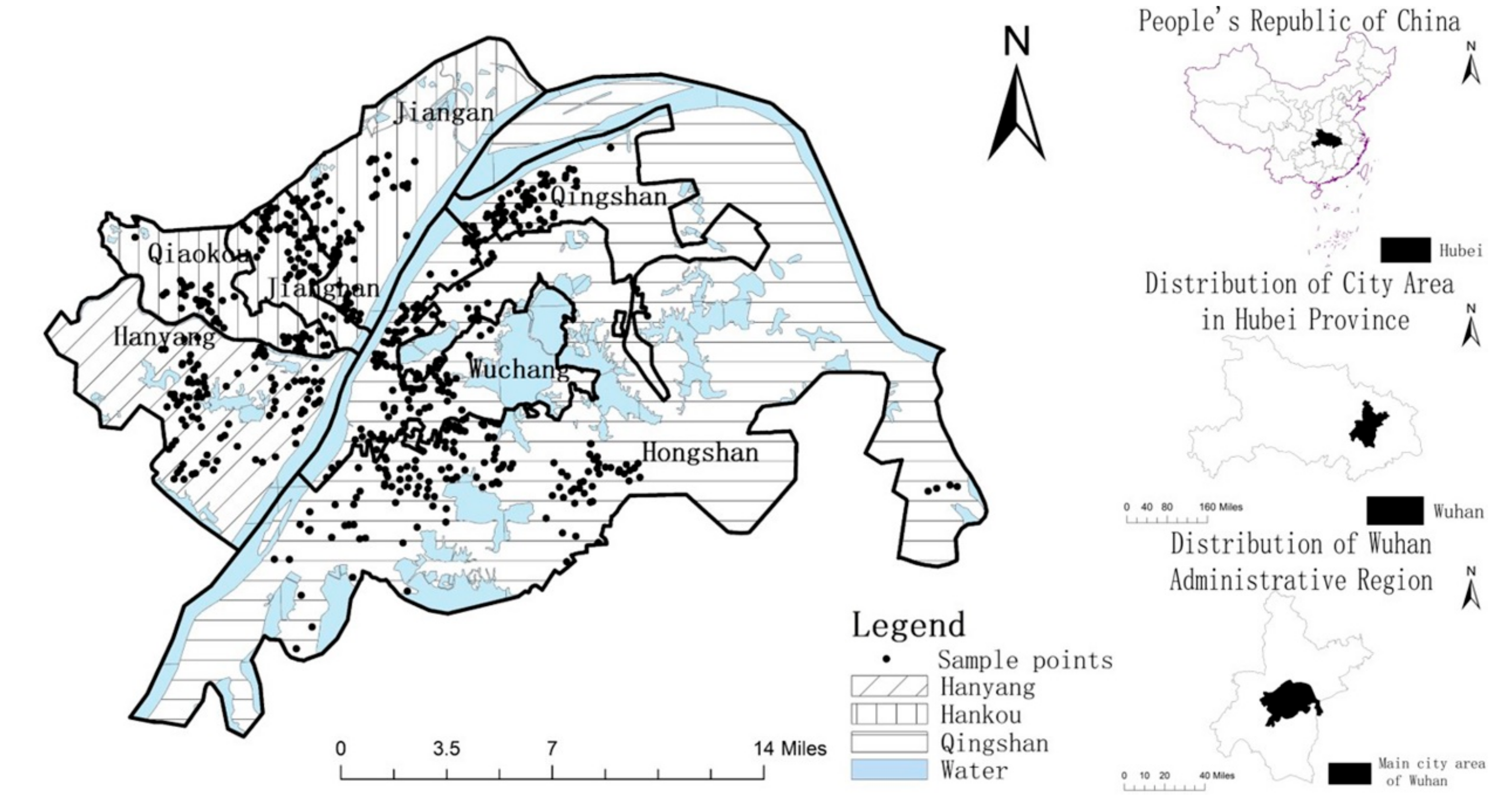
As the capital of Hubei Province, Wuhan is the largest mega-city in central China and in the middle reaches of Yangtze River. The Yangtze River and the Han River converge in the center of the city and divide Wuhan into three parts: Wuchang, Hankou and Hanyang. Respectively, the three parts function as the educational and cultural center, the commercial and financial center as well as the industrial center of Wuhan, which makes Wuhan distinct as a polycentric city. The main city area of Wuhan consists of seven administrative districts. Among them: Jianghan district, Jiang’an district and Qiaokou district are in the part of Hankou; Hanyang district is the core area of Hanyang; and Wuchang, Hongshan, and Qingshan district belong to Wuchang (Figure 1). In this study, the main city area was selected for the following reasons: Firstly, this region has the densest population and most urbanization area. Secondly, this region also has more complex urban infrastructure development, including the densely distributed metro lines and stations, abundant urban green space and social facilities such as schools, hospitals and central business districts (CBDs). Thirdly, this region includes the core area of the three functional centers. With these considerations in mind, we select the seven main city districts to carry out a comprehensive analysis of the space-time distribution pattern of housing prices and their influencing factors.
2.2. Datasets and Variables
In this paper, we carry out the research from the perspective of the community level. Since second-hand apartments are considered to be more market-oriented in China and more suitable for reflecting the personal preferences of urban infrastructure [9], we used the average price of second-hand apartments (in Yuan/) of residential communities as the dependent variable. Due to the lack of transaction datasets of second-hand apartments from statistical authorities, we developed a web-crawling tool to assemble housing transaction dataset from anjuke.com, which is a real estate broker platform in China. Each residential community sample contains the attribute information such as the community name, address, monthly average price, green rate, volume ratio, etc. With the data verification from the two other major real estate transaction websites (Fangtianxia and HomeLink), finally 619 residential community records with complete information were sorted out as research samples in the main urban areas of Wuhan from 2010 to 2018. After using Google Earth to obtain the spatial location information of each residential community, the distribution of these residential communities is shown in Figure 1. We also used the web-crawling program to collect urban facilities information on location sites of bus stops, metro stations, hospitals, CBDs, schools and city parks and scenery based on the point of interest (POI) services of Baidu Map (map.baidu.com), which we then complemented and verified using Google Earth’s satellite maps. Then ArcGIS software was used to visualize the geographical factors such as the administrative division boundary, traffic network and river system of Wuhan’s main city area, and finally a spatial attribute database of the residential communities in the research area was established.
To examine the effects of urban facilities on housing prices at the community level, we extended the hedonic price model with GTWR, which enabled us to explore various mechanisms operating across space and time. A total of 11 influential factors of housing prices were selected, which were residential community structure attributes, urban physical infrastructure and social infrastructure. Table 1 shows more details about these independent variables.
Since the multicollinearity problem causes unstable results, the tool of Variance Inflation Factor was used to detect the multicollinearity among variables before building the regression models. The results showed that the VIF value of each explanatory variable was far less than 10, indicating that there is no obvious multicollinearity among explanatory variables and the selected variables are suitable for further regression analysis.
2.3. Methods
2.3.1. Kriging Spatial Interpolation
Spatial interpolation refers to the method of calculating the data of other uncollected points in the same region through the data of known sample points. In the spatial interpolation methods, Kriging interpolation is an accurate local interpolation method, which is based on spatial autocorrelation and uses the structure of a semi-variogram to make an unbiased optimal estimation of the value of regionalized variables in a finite area [23]. It is a precise local interpolation method, which not only considers the distance between the sample points, but also considers the spatial distribution of the known sample points and the spatial orientation of the unknown sample points through analysis of the variation function and structure. Moreover, it makes use of the structural characteristics of the spatial distribution of the existing observation values to make the estimation results more accurate than the traditional methods and avoid the occurrence of systematic errors more effectively. The formula is:
where Z () is the value of the predicted position, Z () is the measured value of position i, is the weight coefficient of position i, and n is the number of sample points.
2.3.2. GTWR Model
The GTWR model extends the traditional GWR model by combining spatial position coordinates with time series coordinates to form three-dimensional coordinates, creating conditions for analyzing the spatial and temporal characteristics of regression relations. In this paper, the GTWR model has been applied for hedonic price modeling, which commonly includes three forms of functions: linear, semi-logarithmic, and logarithmic. After continuous trials and comparisons, this paper uses a logarithmic form to build the model. The specific forms of the equation are as follows:
where i is the index of a spatial-temporal point with denoting its coordinates. Accordingly, ,, are the dependent variable, the jth independent variable, and the error term for the ith observation (point), respectively.
In the analysis of spatio-temporal data, the closer the sample data point is to any point () in the study area, the greater the influence on the parameter estimation at (). The space-time distance between point () and the sample data point () is measured by "d". The larger the weight value, the smaller the distance assigned to a smaller weight value accordingly. Given a spatial distance and a temporal distance , we could combine them to form a spatio-temporal distance such that
where λ and μ are scale factors to balance the different effects used to measure the spatial and temporal distance in their respective metric systems. Therefore, if the parameters λ and μ are adjusted appropriately, then can be used to measure the extent of ‘closeness’ in a spatio-temporal space. It can be proved that when the Gaussian kernel function is selected, the above definition guarantees the separability of the space-time weight matrix. Thus, it follows that we can build a spatially weighted matrix and a temporally weighted matrix and then combine them to form a spatio-temporal weight matrix .
The basic principle is to set the weight by the distance between each data point j and the regression point i, and use a function to express the relationship between the weight between the two points and the distance, the expression is as follows:
where b is the bandwidth of the spatio-temporal weight function, and the size of the bandwidth directly affects the spatio-temporal change of the GTWR model. According to the evaluation criteria proposed by Fotheringham [25], when the model’s AICc is the smallest, its bandwidth b is the best. LuBinbin et al. [45] further showed that the smaller the AICc value is, the higher the model’s accuracy becomes. If the AIC value difference between different models exceeds 3, then the model with a lower AICc value will be regarded as a better model. At the same time, the model’s Residual Squares () can also reflect the strength of the model. It is generally believed that the higher the model’s , the better the fit of the model.
3. Spatio-Temporal Pattern of Housing Prices
3.1. Time Evolution
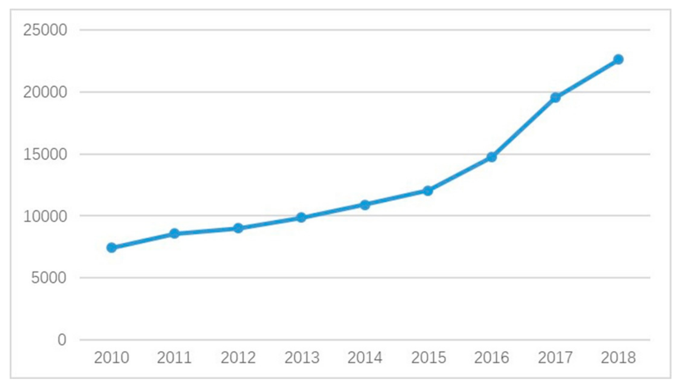
The average prices of residential communities in the main city area of Wuhan from 2010 to 2018 are shown in Figure 2. It shows that the housing prices of residential communities are generally on the rise, but the increment speed shows an obvious periodic characteristic. During the 9 years, the average price of residential communities in the main city area of Wuhan increased from 7445.706Yuan/ to 22629.37 Yuan/, with an average annual increase of 1687.074 Yuan/. The price increased by 203.9925% and the average annual increase was 14.907%. Among them, the increase was slower from 2010 to 2015, with an average annual increase of only 918.999 Yuan/, with an average annual increase of 10.09%; from 2015 to 2017, it rose rapidly, with an annual increase of 27.328%. In 2018, the increase rate reduced, and the lower increase rate was 15.923%.
3.2. Spatial Distribution
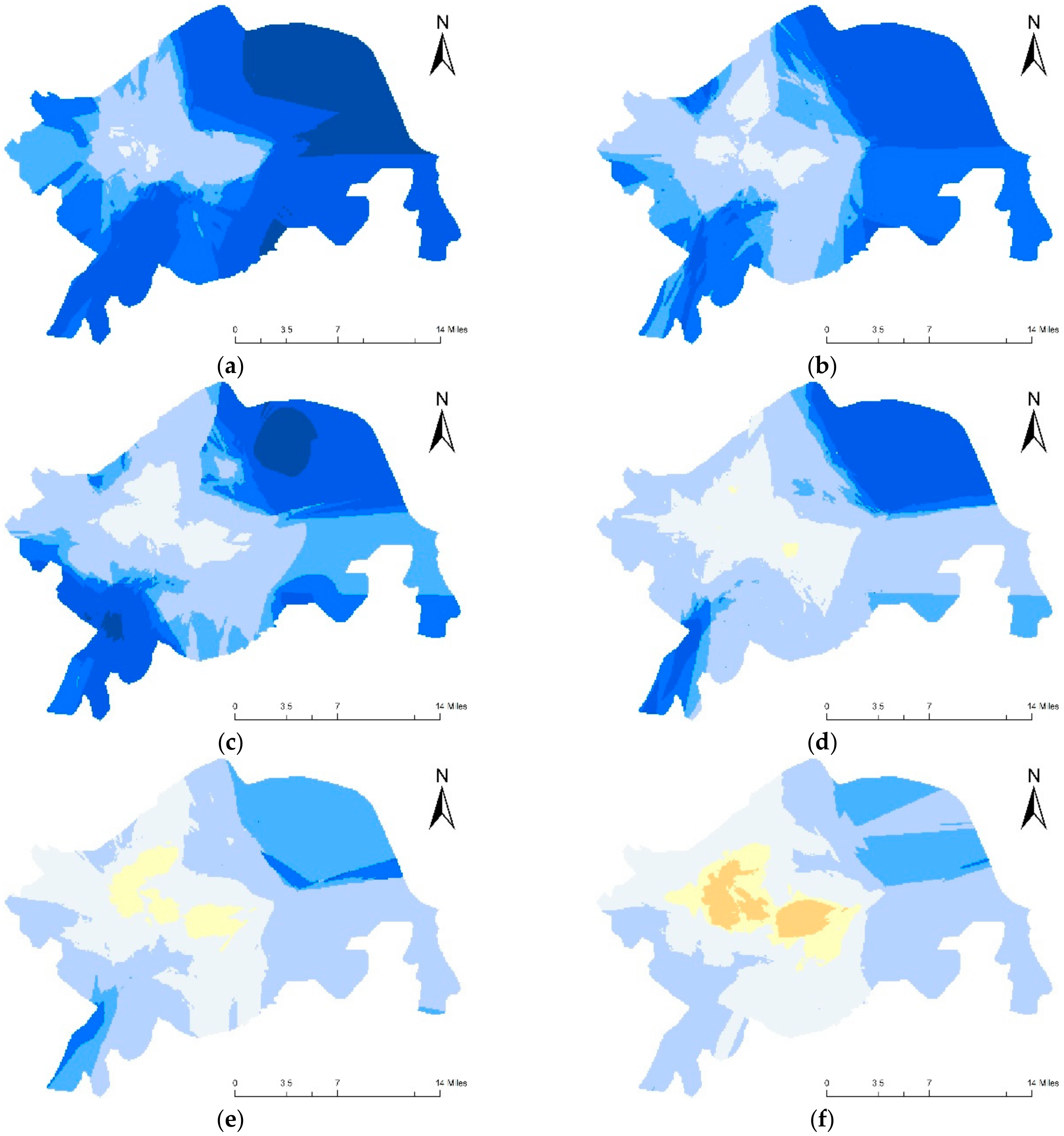
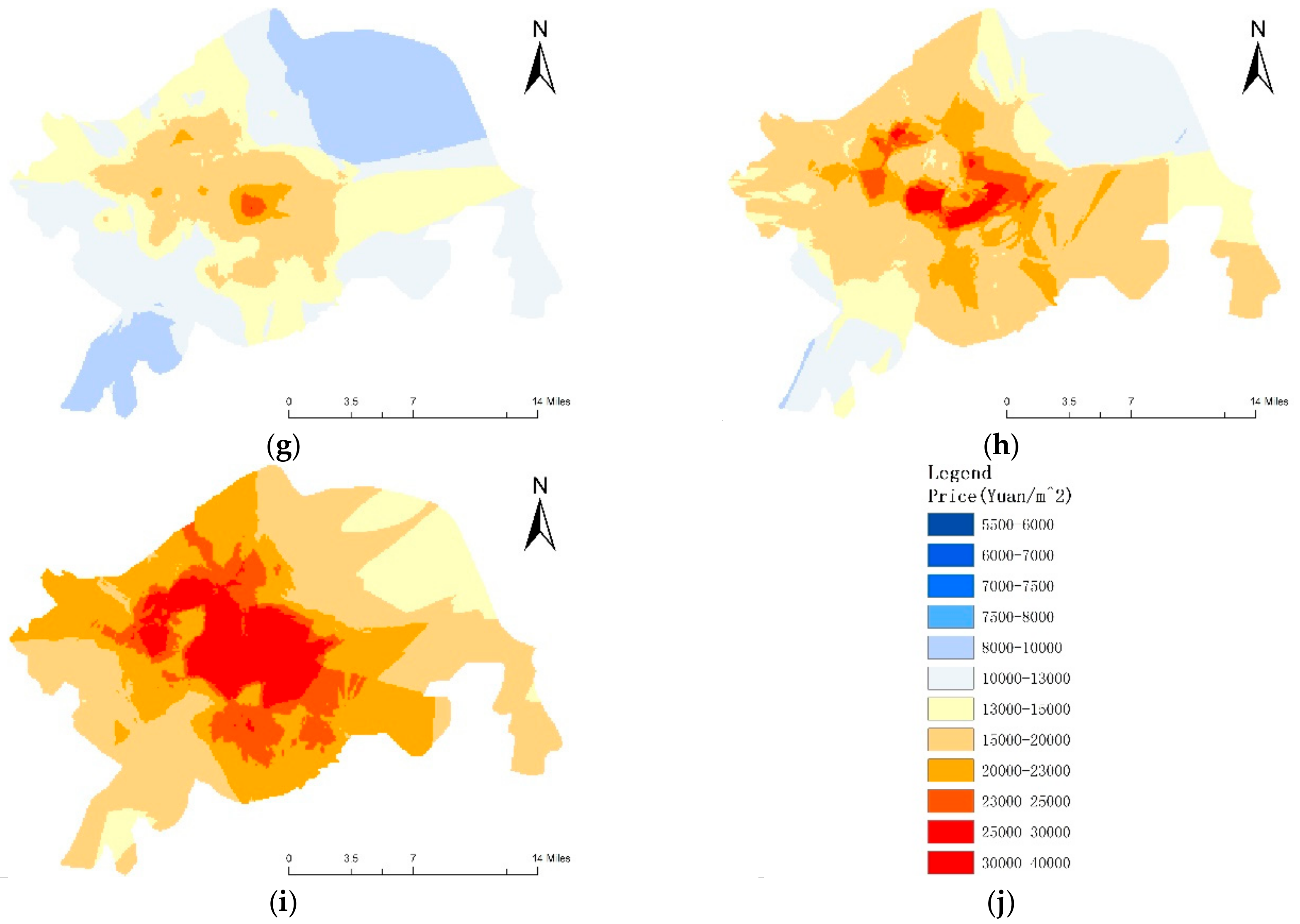
By using kriging interpolation in Arc GIS10.2, the spatial pattern of housing prices in the main urban area of Wuhan from 2010 to 2018 was analyzed, which is shown in Figure 3. The results show that:
- (1)
- The spatial pattern shows a significant multiple core-periphery distribution.
The prices of residential communities have formed the high-value clusters in the three core areas of the main city area and gradually decreases to the periphery. Using the Baidu electronic map, the high-value concentration areas of housing prices were identified to be mainly located in Zhongshan Park and Yanjiang Avenue in Jianghan district, Jiefang Park in Jiangan district and Shahu Park, Zhongbei Avenue, and East Lake in Wuchang district.
- (2)
- The peak value area of residential communities shifted from Hankou to Wuchang gradually.
In 2010, the highest value community was distributed in Zhongshan Park in Jianghan and Jiefang Park within the Jiang’an district in Hankou, while in 2018 the housing prices around East lake in Wuchang district had the highest values. The East Lake scenic area is one of the best ecological environment areas in Wuhan. The shift of the peak value may be related to residents’ increasing preference for not only living in a convenient location but also in a superior ecological environment [46].
- (3)
- Housing prices are sensitive to the spatial differences of urban facility distributions.
The spatial distribution of housing prices in the main city area of Wuhan is closely related to the distribution of various urban facilities. The high value of housing prices is mainly concentrated in the surrounding areas of major commercial centers and convenient transportation areas, along the major water system, and urban recreational locations in the core areas.
4. Effects of Urban Facilities on Housing Prices
4.1. Model Comparison
At this stage, three regression models were built and compared to find the best model to fit the dataset. Firstly, the hedonic price model (HPM) based on ordinary least squares (OLS) regression was built in linear, semi-logarithmic, and logarithmic forms, respectively. After comparing them, the logarithmic form was found to be better than the other two forms. The results are displayed in Table 2. The results showed that the model is statistically significant and 39.63% of the variation in the housing prices can be explained by the model according to . Then, before the GWR model and GTWR model were constructed to respectively explore the spatial non-stationarity and spatiotemporal heterogeneity, the spatial and temporal non-stationarity were tested using the statistical value proposed by Leung [47]. According to the F-test criterion, we can judge whether a parameter has passed the test based on the p-value. Table 3 lists the F-statistics value of each variable and its corresponding p-value in the GWR model and GTWR model. The results in Table 3 show obvious spatial variation in the GWR model and spatio-temporal non-stationarity in the GTWR model. Furthermore, by comparing the performance of the traditional hedonic model and the GWR and GTWR models (Table 4), we can conclude that GTWR outperforms OLS and GWR model in terms of model fit. In particular, the adjusted increases from 0.3728 in the OLS model and 0.5568 in the GWR model to 0.8879 in the GTWR model. Also, the AIC value of GTWR experienced the smallest variable increase in all three models. So, it can be inferred that GTWR significantly increases the explanatory power while considering both spatial and temporal heterogeneities.
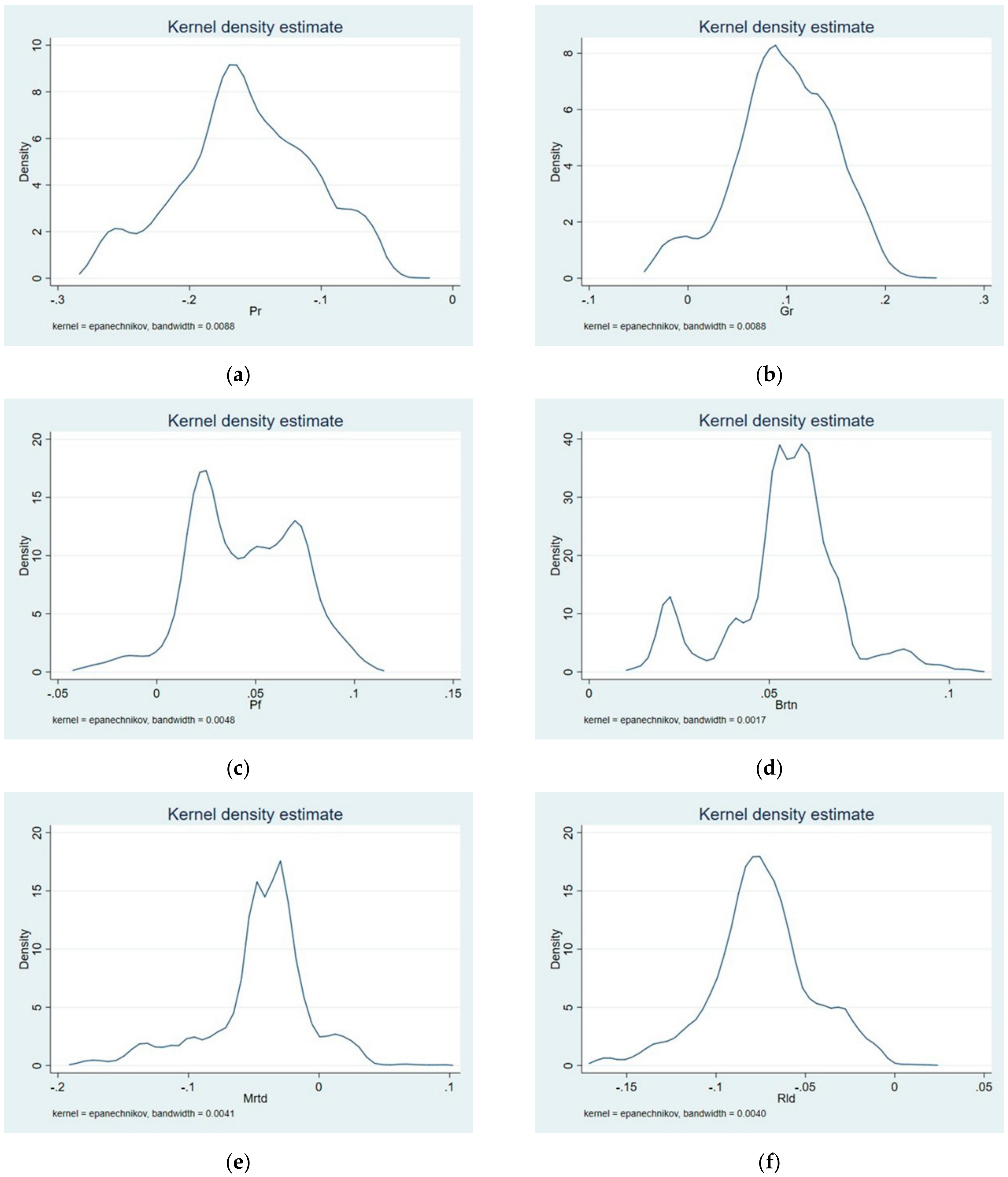
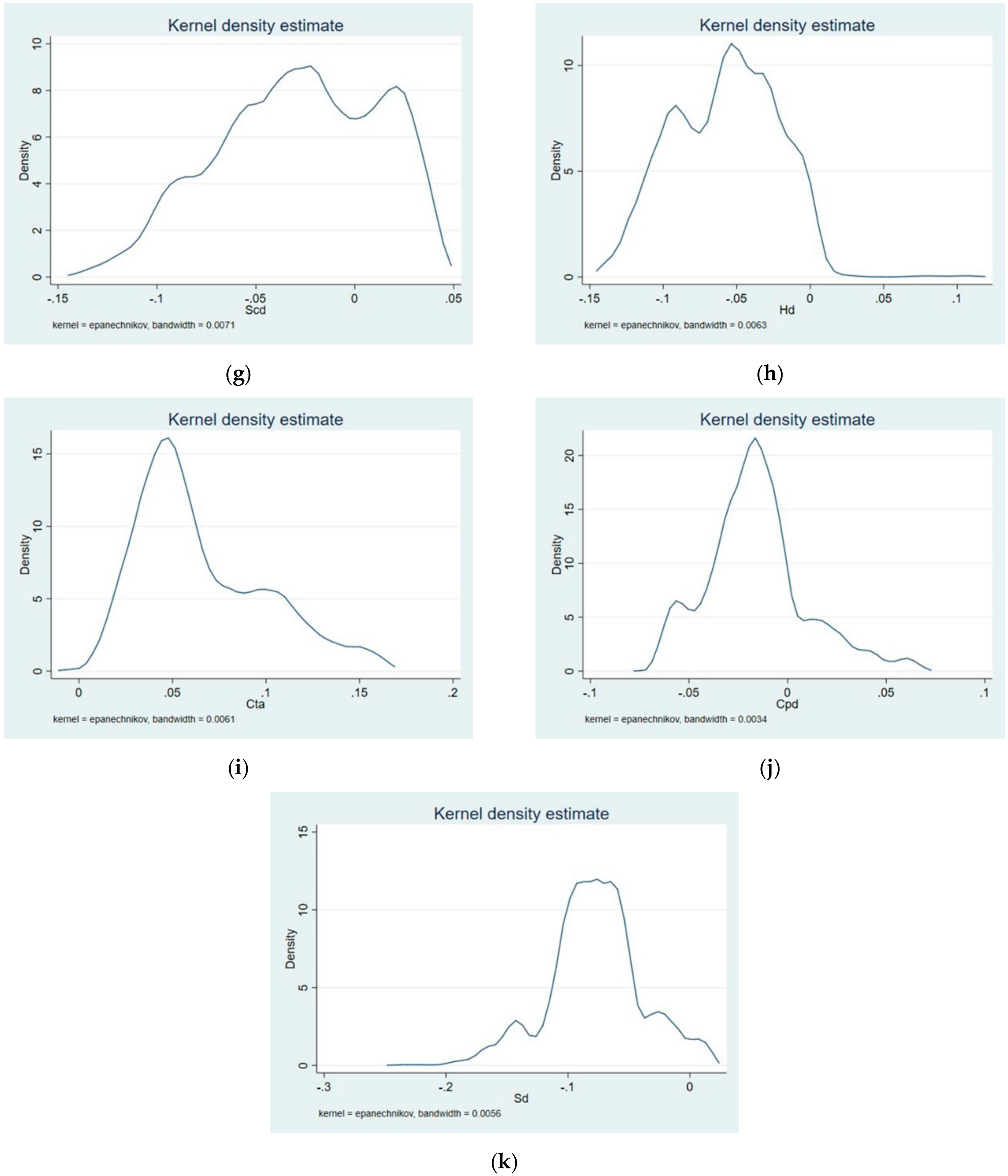
Because the outputs of local parameter estimates from GTWR would be voluminous, Table 5 only provides quantile statistics and mean value of each parameter distribution to indicate the extent of its variability. Based on the GTWR regression results in Table 5, the sign of the average coefficient of plot ratio, the distance to the nearest MTR station, the nearest river and lake, the nearest large shopping center, the nearest top three hospitals, the nearest city park, and both primary and secondary schools are all negative, which indicates that increasing their densities or distance from houses will generally decrease the prices of these houses. The sign of green rates, property fees, number of bus routes, and the distance to the nearest cultural tourist attractions are positive, thereby suggesting that housing prices will increase when increasing green areas, property management fees, bus routes numbers, and the accessibility of cultural tourist attractions. To better visualize the effects, a kernel density map of the regression coefficients of each variable factor was drawn (Figure 4). From the kernel density map, it could be observed that the distribution of the regression coefficients of different influence factors was significantly different.
4.2. Spatial Feature of Coefficients
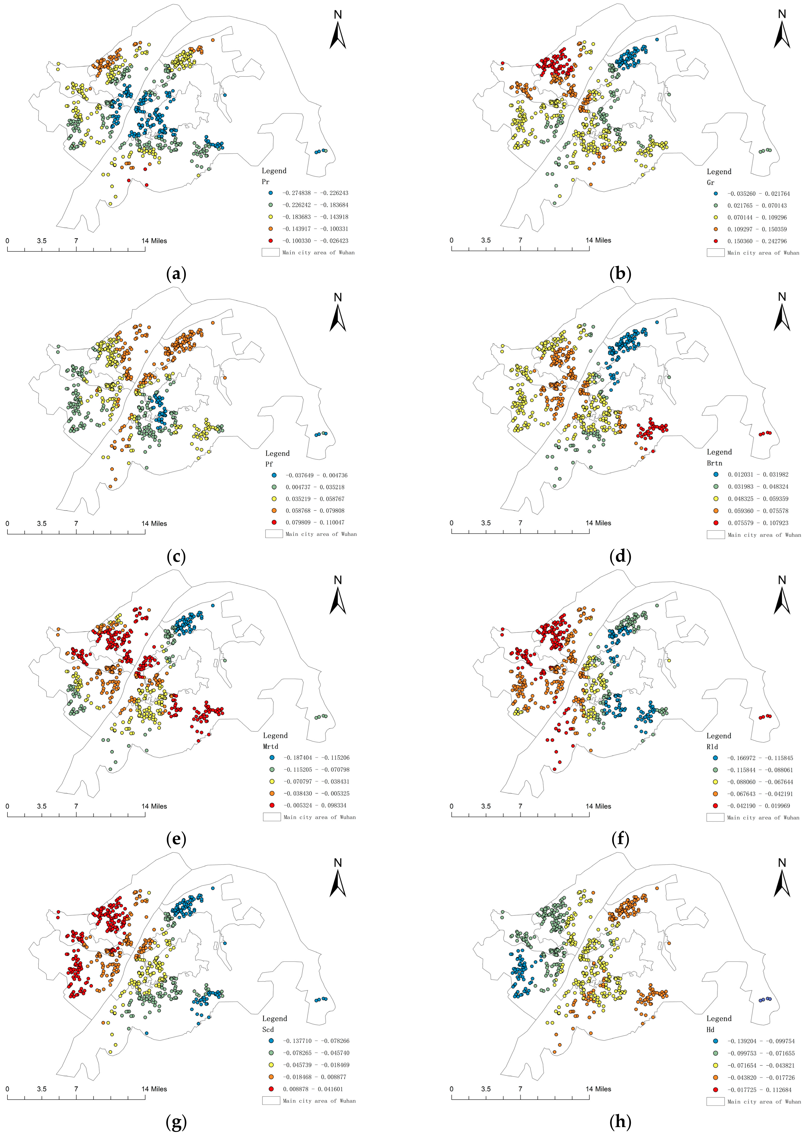
The remarkable feature of the GWR series model is that the coefficient variation can be graphically analyzed. The characteristics of the stability change of each influence factor were analyzed by plotting the coefficient change characteristics of the GTWR, and the spatial pattern difference and order dynamic change were analyzed (Figure 5).
- (1)
- Structural Characteristic Factor Analysis
In Figure 5, sub-figure (a–c) show the spatial distribution of the coefficient of residential community structure characteristics. The spatial distribution of the coefficients in sub-figure (a–c) decrease gradually from the core area to the peripheral area. The coefficients of the three structural attributes in the core areas of Hankou and Wuchang are bigger than that in the peripheral area, thereby indicating that the better the development level of residential community, the greater the correlation that exists between its price and structural characteristics. The reason for this may be that the higher-end residential communities concentrate more in the core area where the residents generally have higher incomes and consumption capacities, who usually pay more attention to the internal environmental conditions of the residential areas to pursue more comfortable living environments.
- (2)
- Impact of Urban Physical Infrastructure
In Figure 5, sub-figure (d–e) show the spatial variation of the coefficients of public physical facilities, indicating that housing prices are affected by the degree of transportation convenience around the residence. However, the impact strength varied depending on the transport type and different area. In the peripheral area where subway stations are sparsely distributed, local housing prices are greatly affected by the subway station, while the number of bus lines has a relatively small impact on housing prices. In the core areas where the public transportation network is well developed, the influence of subway stations decreased, while the influence of the number of bus routes increased compared with that in the peripheral area. This indicates that metro rail transit has no special advantage over short-distance travel.
Sub-figure (f) shows the spatial variation of the distance parameter from the residence to the nearest river and lake. The experimental results show that green urban infrastructure, such as rivers and lakes, generally has a negative effect on prices, which shows that the closer the distance to the water area is, the higher the housing prices will be. The spatial distribution of its coefficient is closely related to the spatial distribution of rivers and lakes in Wuhan, and presents significant regional differences. Among those rivers and lakes, the coefficient values around Yangtze river, South Lake, East Lake, and Sand Lake are higher, indicating that these rivers and lakes have the strongest promoting effect on the increase of housing prices around them.
- (3)
- Effect of Urban Social Facilities
In Figure 5, sub-figure (g) shows the spatial variation of the effect of commercial facilities on housing prices. In Qingshan district and Hongshan district the coefficients have higher values where shopping centers are more sparsely distributed. The closer a house is to the large shopping center, the more convenient it is for its residents to live and shop there. Therefore, a large shopping mall can promote the increase of housing prices in surrounding areas to a certain extent. However, the dense existence of large shopping malls inevitably has negative effects such as traffic congestion and noise pollution, so the housing prices of a residential community which is too close to the dense shopping centers will be relatively low. Therefore, the Jianghan Road Commercial Center and Aviation Road Commercial Center have a negative impact on the housing prices of nearby communities in Jianghan District. In general, large shopping malls and commercial streets can promote the increase of housing prices in the surrounding areas, as long as the houses are not too close to the densely distributed large shopping malls.
Sub-figure (h) shows the spatial variation of distance parameters to the nearest top three hospitals. On the whole, the regression coefficient of medical resources shows a trend of increasing gradually from the periphery to the core areas, revealing that the influence of medical facilities on housing prices in fringe areas is greater than that in the core areas, which may be the result of the unequal distribution of medical resources.
Sub-figure (i) shows the spatial variation of the distance parameter to the nearest famous tourist attraction. The coefficient decreases from the center of the main city area to the periphery, and Wuchang district becomes the gathering area of positive and high values. Wuhan’s famous cultural tourist attractions mainly include a celebrity memorial hall and historical sites, which are mainly distributed in the Wuchang district. The existence of tourist attractions is bound to lead to a large number of tourists, which increases traffic congestion, environmental damage, and other negative effects, meaning that housing near famous tourist attractions areas, such as Wuchang district, will be negatively affected significantly in terms of their prices.
Sub-figure (j) shows the spatial variation of the distance parameter to the nearest park. The distance parameter between the price of second-hand housing and a park is generally negative. The negative high value of the coefficient is mainly distributed in the core areas of the main urban area and spreads to the surrounding areas., It indicates that the effect of city parks is more sensitive in the Jiang’an, Jianghan, Qiaokou, and Wuchang districts, which have more dense construction and small green areas around residential buildings than in the peripheral area, which has widely distributed and larger green areas.
Sub-figure (k) shows the spatial variation of distance parameters to the nearest key primary and secondary schools, and the coefficient distribution presents significant spatial differences. The negative high values are concentrated in the peripheral areas of the main city area with a sparse distribution of key primary and secondary schools, such as Hongshan district, while the effect of education facilities is relatively low in some areas with adequate educational resources, such as Qingshan district and Wuchang district.
4.3. Temporal Feature of Coefficients
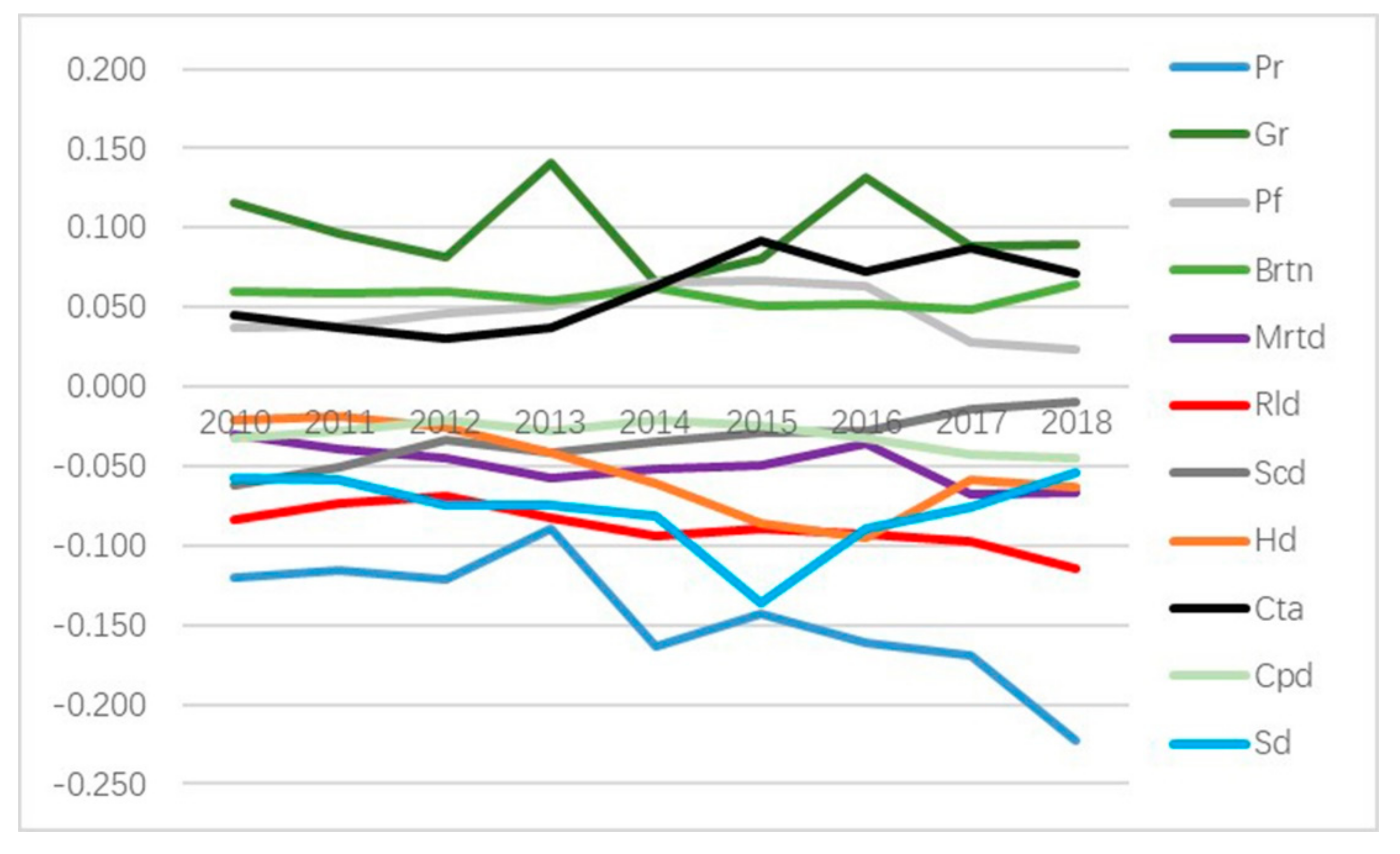
In order to show the time series fluctuation of each influence factor, this paper calculated the mean value of the influence factor coefficients of each year to draw the trend chart of influence factor coefficients. The results are displayed in Figure 6. It shows that, from 2010 to 2018, the influential intensity of each influential factor on the housing prices varies, but the influential intensity trends can be generally divided into three categories: increasing, decreasing, and basic stability. The effects intensity of the nearest river and lake as well as the nearest city park has been increasing steadily in the past 9 years. The influences of plot ratio, the nearest top three hospitals, MRT, and cultural tourist attractions has increased on a fluctuating basis. The increasing influences of the above influential factors indicates that urban residents are paying more attention to the convenience of commuting, the superiority of surrounding landscapes, and the comfort of community life. However, the influences of large shopping malls and commercial streets and greenery rates in the community on the housing price are decreasing, which indicates that with urbanization, the welfare provided by traditional commercial facility and greenery rates in the community could be provided by other urban facilities. The rest of influencing factors all show a state of fluctuation but also long-term stability during the whole study period.
5. Conclusion and Discussion
This paper takes the main urban area of Wuhan city as an example, constructs a GTWR model with coupling spatial heterogeneity and time non-stationarity,, and selects structural characteristics of a residential community, physical urban infrastructure, and social infrastructure to explore the spatial and temporal differentiation patterns and influencing factors on housing prices in the main city area of Wuhan from 2010 to 2018. The conclusions are as follows:
- (1)
- The prices of residential communities in the main city area of Wuhan have been on the rise from 2010 to 2018, but the speed of this increase has slowed down. From 2010 to 2015, the price of second-hand residential buildings has been rising slowly, with an average annual increase of 10.09%. From 2015 to 2017, the price of second-hand housing rose rapidly, with an annual increase of 27.328%. In 2018, however, the rate of increase in home prices tended to slow down, rising at a lower rate of 15.923%.
- (2)
- Housing prices in the main city area of Wuhan has a multiple core-peripheral distribution. The peak value of housing prices shifted from the core areas in Hankou to Wuchang. The spatial dynamic distribution of housing prices is sensitive to the development of urban infrastructure.
- (3)
- Compared with the OLS and GWR models, GTWR has a better fit and simulation accuracy, which verifies the applicability of the GTWR model in housing price research. The GTWR results show that the influence of urban facilities on housing prices has significant temporal and spatial non-stationarity. Spatially, the influence factors show different differentiation rules in spatial distribution, and the influencing direction and strength of the urban infrastructure on housing prices are closely related to the spatial location, distribution density, and the type of urban infrastructure. Temporally, the influencing strength of various urban facilities varies. Among all the urban facility factors, only the influence of commercial facilities decreased, while the effects of most of urban facilities kept increasing or were stable overall.
Based on our research results, we found that housing prices are affected by a city’s structure. However, the spatial distribution can be affected by urban facilities development. Generally, the impact strength increases, but the specific impact direction and strength of each variable varies. For example, an MRT cause increased housing prices but this trend would be more obvious in the periphery areas than in the core areas in Wuhan. Shopping centers had a stronger influence on housing prices in 2010 than in 2018, while rivers and lakes showed the opposite influence trend. At the same time, we learned from Wesołowska’s research that the location and construction process of new public investments of urban infrastructure leads to numerous protests by inhabitants of local communities [44]. One of the advantages of the GTWR model is that it can visually see the spatiotemporal differentiation characteristics of each influence factor. Therefore, based on this advantage, we can analyze the spatial and temporal influence characteristics of urban infrastructure on the surrounding area, so as to provide references for the layout of various urban infrastructure, reduce the time cost of selecting suitable locations for urban infrastructure layout, as well to engage with local inhabitants’ concerns about surrounding environmental pollution and decreases to their property values. All of these findings show that housing demands vary with the spatio-temporal development of urban infrastructure, and that the GTWR model can be a useful tool to discover the factors influencing housing prices, which may help urban planners to optimize urban facilities to promote the sustainable development of Wuhan, as well as policy-makers when formulating more specific housing policies.
However, this paper still has some limitations. First, our study mainly depends on the proximity between the residential community and urban facilities based on the Euclidean distance. However, accessibility also plays an important role in geographical accessibility, which was neglected in our study. Second, the selected urban facility variables are limited. For example, we did not include industrial facilities [48] and we also did not further differentiate the amenity variables among urban facilities. Future research can explore these areas.
Author Contributions
M.M. conceptualized the framework of this study and determined the method. F.L. contributed to the methodology, data collection, data processing, and result analysis. K.Z. and W.H. provided some valuable comments and revised the original manuscript. All authors have read and agreed to the published version of the manuscript.
Funding
This research was funded by “the Fundamental Research Funds for the Central Universities”, Huazhong Agricultural University (2662019FW017), the National Natural Science Foundation of China (71103072) and the Major Project of National Social Science Foundation of China (18ZDA054).
Acknowledgments
We thank the anonymous referees for their comments on the paper. All of the errors and omissions remain our own.
Conflicts of Interest
The authors declare no conflict of interest.
References
- Kang, H.-H.; Liu, S.-B. The impact of the 2008 financial crisis on housing prices in China and Taiwan: A quantile regression analysis. Econ. Model. 2014, 42, 356–362. [Google Scholar] [CrossRef]
- Liang, W.; Lu, M.; Zhang, H. Housing prices raise wages: Estimating the unexpected effects of land supply regulation in China. J. Hous. Econ. 2016, 33, 70–81. [Google Scholar] [CrossRef]
- Wang, Y.; Wang, S.; Li, G.; Zhang, H.; Jin, L.; Su, Y.; Wu, K. Identifying the determinants of housing prices in China using spatial regression and the geographical detector technique. Appl. Geogr. 2017, 79, 26–36. [Google Scholar] [CrossRef]
- Lan, F.; Gong, X.; Da, H.; Wen, H. How do population inflow and social infrastructure affect urban vitality? Evidence from 35 large- and medium-sized cities in China. Cities 2019, 102454. [Google Scholar] [CrossRef]
- Lu, J. The value of a south-facing orientation: A hedonic pricing analysis of the Shanghai housing market. Habitat Int. 2018, 81, 24–32. [Google Scholar] [CrossRef]
- Xiao, Y.; Hui, E.C.M.; Wen, H. Effects of floor level and landscape proximity on housing price: A hedonic analysis in Hangzhou, China. Habitat Int. 2019, 87, 11–26. [Google Scholar] [CrossRef]
- Choy, L.H.T.; Mak, S.W.K.; Ho, W.K.O. Modeling Hong Kong real estate prices. J. Hous. Built Environ. 2007, 22, 359–368. [Google Scholar] [CrossRef]
- Liang, X.; Liu, Y.; Qiu, T.; Jing, Y.; Fang, F. The effects of locational factors on the housing prices of residential communities: The case of Ningbo, China. Habitat Int. 2018, 81, 1–11. [Google Scholar] [CrossRef]
- Li, H.; Wei, Y.D.; Wu, Y.; Tian, G. Analyzing housing prices in Shanghai with open data: Amenity, accessibility and urban structure. Cities 2019, 91, 165–179. [Google Scholar] [CrossRef]
- Yuan, F.; Wei, Y.D.; Wu, J. Amenity effects of urban facilities on housing prices in China: Accessibility, scarcity, and urban spaces. Cities 2020, 96, 102433. [Google Scholar] [CrossRef]
- Cordera, R.; Chiarazzo, V.; Ottomanelli, M.; dell’Olio, L.; Ibeas, A. The impact of undesirable externalities on residential property values: Spatial regressive models and an empirical study. Transp. Policy 2019, 80, 177–187. [Google Scholar] [CrossRef]
- Gao, Y.; Tian, L.; Cao, Y.; Zhou, L.; Li, Z.; Hou, D. Supplying social infrastructure land for satisfying public needs or leasing residential land? A study of local government choices in China. Land Use Policy 2019, 87, 104088. [Google Scholar] [CrossRef]
- Cui, Y.; Sun, Y. Social benefit of urban infrastructure: An empirical analysis of four Chinese autonomous municipalities. Util. Policy 2019, 58, 16–26. [Google Scholar] [CrossRef]
- Song, Z.; Cao, M.; Han, T.; Hickman, R. Public transport accessibility and housing value uplift: Evidence from the Docklands light railway in London. Case Stud. Transp. Policy 2019, 7, 607–616. [Google Scholar] [CrossRef]
- Efthymiou, D.; Antoniou, C. How do transport infrastructure and policies affect house prices and rents? Evidence from Athens, Greece. Transp. Res. Part A Policy Pract. 2013, 52, 1–22. [Google Scholar] [CrossRef]
- Seo, W.; Nam, H.K. Trade-off relationship between public transportation accessibility and household economy: Analysis of subway access values by housing size. Cities 2019, 87, 247–258. [Google Scholar] [CrossRef]
- Votsis, A. Planning for green infrastructure: The spatial effects of parks, forests, and fields on Helsinki’s apartment prices. Ecol. Econ. 2017, 132, 279–289. [Google Scholar] [CrossRef] [Green Version]
- Jun, M.-J.; Kim, H.-J. Measuring the effect of greenbelt proximity on apartment rents in Seoul. Cities 2017, 62, 10–22. [Google Scholar] [CrossRef]
- Daams, M.N.; Sijtsma, F.J.; Veneri, P. Mixed monetary and non-monetary valuation of attractive urban green space: A case study using Amsterdam house prices. Ecol. Econ. 2019, 166, 106430. [Google Scholar] [CrossRef]
- Brasington, D.; Haurin, D.R. Educational Outcomes and House Values: A Test of the value added Approach. J. Reg. Sci. 2006, 46, 245–268. [Google Scholar] [CrossRef] [Green Version]
- Franco, S.F.; Macdonald, J.L. The effects of cultural heritage on residential property values: Evidence from Lisbon, Portugal. Reg. Sci. Urban Econ. 2018, 70, 35–56. [Google Scholar] [CrossRef] [Green Version]
- D’Acci, L. Quality of urban area, distance from city centre, and housing value. Case study on real estate values in Turin. Cities 2019, 91, 71–92. [Google Scholar] [CrossRef]
- Martínez, M.G.; Lorenzo, J.M.M.; Rubio, N.G. Kriging methodology for regional economic analysis: Estimating the housing price in Albacete. Int. Adv. Econ. Res. 2000, 6, 438–450. [Google Scholar] [CrossRef]
- Chica-Olmo, J. Prediction of Housing Location Price by a Multivariate Spatial Method: Cokriging. J. Real Estate Res. 2007, 29, 91–114. [Google Scholar]
- Stewart Fotheringham, A.; Charlton, M.; Brunsdon, C. The geography of parameter space: An investigation of spatial non-stationarity. Int. J. Geogr. Inf. Syst. 1996, 10, 605–627. [Google Scholar] [CrossRef]
- Fotheringham, A.; Brunsdon, C.; Charlton, M. Geographically Weighted Regression: The Analysis of Spatially Varying Relationships; Wiley: Chichester, UK, 2002. [Google Scholar]
- Kestens, Y.; Thériault, M.; Des Rosiers, F. Heterogeneity in hedonic modelling of house prices: Looking at buyers’ household profiles. J. Geogr. Syst. 2006, 8, 61–96. [Google Scholar] [CrossRef]
- Lu, B.; Charlton, M.; Fotheringhama, A.S. Geographically Weighted Regression Using a Non-Euclidean Distance Metric with a Study on London House Price Data. Procedia Environ. Sci. 2011, 7, 92–97. [Google Scholar] [CrossRef] [Green Version]
- Holly, S.; Pesaran, M.H.; Yamagata, T. A spatio-temporal model of house prices in the USA. J. Econom. 2010, 158, 160–173. [Google Scholar] [CrossRef]
- Hu, S.; Yang, S.; Li, W.; Zhang, C.; Xu, F. Spatially non-stationary relationships between urban residential land price and impact factors in Wuhan city, China. Appl. Geogr. 2016, 68, 48–56. [Google Scholar] [CrossRef] [Green Version]
- Huang, B.; Wu, B.; Barry, M. Geographically and temporally weighted regression for modeling spatio-temporal variation in house prices. Int. J. Geogr. Inf. Sci. 2010, 24, 383–401. [Google Scholar] [CrossRef]
- Cohen, J.P.; Coughlin, C.C.; Zabel, J. Time-Geographically Weighted Regressions and Residential Property Value Assessment. J. Real Estate Financ. Econ. 2020, 60, 134–154. [Google Scholar] [CrossRef] [Green Version]
- Jin, C.; Lee, G. Exploring spatiotemporal dynamics in a housing market using the spatial vector autoregressive Lasso: A case study of Seoul, Korea. Trans. GIS 2019, 24, 27–43. [Google Scholar] [CrossRef]
- Liu, J.; Yang, Y.; Xu, S.; Zhao, Y.; Wang, Y.; Zhang, F. A Geographically Temporal Weighted Regression Approach with Travel Distance for House Price Estimation. Entropy 2016, 18, 303. [Google Scholar] [CrossRef]
- Wu, C.; Ren, F.; Hu, W.; Du, Q. Multiscale geographically and temporally weighted regression: Exploring the spatiotemporal determinants of housing prices. Int. J. Geogr. Inf. Sci. 2019, 33, 489–511. [Google Scholar] [CrossRef]
- Liu, G.; Wang, X.; Gu, J.; Liu, Y.; Zhou, T. Temporal and spatial effects of a ‘Shan Shui’ landscape on housing price: A case study of Chongqing, China. Habitat Int. 2019, 94, 102068. [Google Scholar] [CrossRef]
- Zhang, L.; Yi, Y. What contributes to the rising house prices in Beijing? A decomposition approach. J. Hous. Econ. 2018, 41, 72–84. [Google Scholar] [CrossRef]
- Wen, H.; Xiao, Y.; Zhang, L. Spatial effect of river landscape on housing price: An empirical study on the Grand Canal in Hangzhou, China. Habitat Int. 2017, 63, 34–44. [Google Scholar] [CrossRef]
- Chen, Q.; Kamran, S.M.; Fan, H. Real estate investment and energy efficiency: Evidence from China’s policy experiment. J. Clean. Prod. 2019, 217, 440–447. [Google Scholar] [CrossRef]
- Wu, C.; Ye, X.; Du, Q.; Luo, P. Spatial effects of accessibility to parks on housing prices in Shenzhen, China. Habitat Int. 2017, 63, 45–54. [Google Scholar] [CrossRef]
- Yang, L.; Chau, K.W.; Chu, X. Accessibility-based premiums and proximity-induced discounts stemming from bus rapid transit in China: Empirical evidence and policy implications. Sustain. Cities Soc. 2019, 48, 101561. [Google Scholar] [CrossRef]
- Liu, T.; Hu, W.; Song, Y.; Zhang, A. Exploring spillover effects of ecological lands: A spatial multilevel hedonic price model of the housing market in Wuhan, China. Ecol. Econ. 2020, 170, 106568. [Google Scholar] [CrossRef]
- Yuan, F.; Wu, J.; Wei, Y.D.; Wang, L. Policy change, amenity, and spatiotemporal dynamics of housing prices in Nanjing, China. Land Use Policy 2018, 75, 225–236. [Google Scholar] [CrossRef]
- Wesołowska, J. Urban Infrastructure Facilities as an Essential Public Investment for Sustainable Cities—Indispensable but Unwelcome Objects of Social Conflicts. Case Study of Warsaw, Poland. Transp. Res. Procedia 2016, 16, 553–565. [Google Scholar]
- Lu, B.; Charlton, M.; Harris, P.; Fotheringham, A.S. Geographically weighted regression with a non-Euclidean distance metric: A case study using hedonic house price data. Int. J. Geogr. Inf. Sci. 2014, 28, 660–681. [Google Scholar] [CrossRef]
- Jim, C.Y.; Chen, W. Consumption preferences and environmental externalities: A hedonic analysis of the housing market in Guangzhou. Geoforum 2007, 38, 414–431. [Google Scholar] [CrossRef]
- Leung, Y.; Mei, C.; Zhang, W.-X. Statistical Tests for Spatial Nonstationary Based on the Geographically Weighted Regression Model. Environ. Plan. A 2000, 32, 9–32. [Google Scholar] [CrossRef]
- Grislain-Letrémy, C.; Katossky, A. The impact of hazardous industrial facilities on housing prices: A comparison of parametric and semiparametric hedonic price models. Reg. Sci. Urban Econ. 2014, 49, 93–107. [Google Scholar] [CrossRef] [Green Version]
Figure 1.
Study area and sample data.

Figure 2.
Average annual price trend of residential communities in Wuhan.

Figure 3.
Price interpolation of housing prices in Wuhan’s main urban area. (a–i) Price interpolation distribution map of Wuhan’s main urban area from 2010 to 2018. (j) Legend of the price interpolation distribution map.
Figure 3.
Price interpolation of housing prices in Wuhan’s main urban area. (a–i) Price interpolation distribution map of Wuhan’s main urban area from 2010 to 2018. (j) Legend of the price interpolation distribution map.


Figure 4.
Regression coefficient distribution density map of each impact factor. (a) Density map of Pr. (b) Density map of Gr. (c) Density map of Pf. (d) Density map of Brtn. (e) Density map of Mrtd. (f) Density map of Rld. (g) Density map of Scd. (h) Density map of Hd. (i) Density map of Cta. (j) Density map of Cpd. (k) Density map of Sd.


Figure 5.
Spatial differentiation map of influential factors. (a) Spatiotemporal variations of Pr. (b) Spatiotemporal variations of Gr. (c) Spatiotemporal variations of Pf. (d) Spatiotemporal variations of Brtn. (e) Spatiotemporal variations of Mrtd. (f) Spatiotemporal variations of Rld. (g) Spatiotemporal variations of Scd. (h) Spatiotemporal variations of Hd. (i) Spatiotemporal variations of Cta. (j) Spatiotemporal variations of Cpd. (k) Spatiotemporal variations of Sd.


Figure 6.
Temporal variation map of influential factors.


Table 1.
Factors affecting housing prices in Wuhan's main district.
| Type | Variable | Abbreviation | Description |
|---|---|---|---|
| Structural Attributes | Plot Ratio | Pr | floor area /covered area |
| Green Rate | Gr | Plot green area/Plot area | |
| Property Fee | Pf | property management fee | |
| Urban physical infrastructure | Public Transport Facilities | Brtn | The number of bus lines included in all bus stops in the 500m buffer zone |
| Mrtd | Euclidean distance to the nearest MTR station | ||
| Urban Green infrastructure | Rld | Euclidean distance to the nearest river and lake | |
| Urban social infrastructure | Commercial Facilities | Scd | Euclidean distance to the nearest large shopping mall |
| Medical Facilities | Hd | Euclidean distance to the nearest top three hospitals | |
| Recreational Facilities | Cta | Euclidean distance to the nearest cultural tourist attractions | |
| Cpd | Euclidean distance to the nearest city park | ||
| Educational Facilities | Sd | Euclidean distance to the nearest key primary and secondary school |
Table 2.
Parameter estimation summary of hedonic price model based on OLS.
| Variables | Coefficient | t-Statistic | t-Probability | 95% Confidence | Interval |
|---|---|---|---|---|---|
| Intercept | 4.5022 | 370.8600 | 0.000000 | 4.2691 | 4.7353 |
| Pr | −0.1506 | −21.3152 | 0.000000 | −0.2255 | −0.0757 |
| Gr | 0.2207 | −35.0200 | 0.000000 | 0.1140 | 0.3274 |
| Pf | 0.1184 | 32.4196 | 0.000000 | 0.0838 | 0.1531 |
| Brtn | 0.0437 | 3.7680 | 0.001000 | 0.0190 | 0.0685 |
| Mrtd | −0.2491 | −27.9652 | 0.000000 | −0.2617 | −0.2364 |
| Rld | −0.0505 | −19.2189 | 0.000000 | −0.0747 | −0.0262 |
| Scd | −0.0094 | −13.8829 | 0.468000 | −0.0347 | 0.0160 |
| Hd | −0.0574 | −41.8826 | 0.000000 | −0.0288 | 0.0859 |
| Cta | 0.0651 | 5.1474 | 0.000000 | 0.0369 | 0.0932 |
| Cpd | −0.0147 | −17.3752 | 0.000000 | −0.0422 | 0.0127 |
| Sd | −0.0120 | −12.0799 | 0.000000 | −0.0387 | 0.0147 |
| Diagnostic information | |||||
| 0.3963 | |||||
| Residual standard error | 0.1304 | ||||
| Residual sum of squares | 0.3963 | ||||
| AICc | −2955.7982 |
Table 3.
Nonstationarity of parameters in the geographically weighted regression (GWR) and geographically and temporally weighted regression (GTWR) models.
Table 3.
Nonstationarity of parameters in the geographically weighted regression (GWR) and geographically and temporally weighted regression (GTWR) models.
| Parameter | GWR | GTWR | ||
|---|---|---|---|---|
| F Value | p-Value | F Value | p-Value | |
| Intercept | 4.30 | 0.0000 | 19.40 | 0.0000 |
| Pr | 2.31 | 0.0100 | 6.18 | 0.0000 |
| Gr | 3.00 | 0.0000 | 12.72 | 0.0000 |
| Pf | 0.88 | 0.2691 | 4.06 | 0.0000 |
| Brtn | 0.23 | 0.0000 | 5.49 | 0.0000 |
| Mrtd | 1.81 | 0.9983 | 11.18 | 0.0000 |
| Rld | 1.08 | 0.0000 | 6.00 | 0.0000 |
| Scd | 0.38 | 0.6532 | 3.14 | 0.0000 |
| Hd | 0.38 | 0.0000 | 1.57 | 0.0214 |
| Cta | 0.94 | 0.3827 | 4.95 | 0.0000 |
| Cpd | 0.96 | 0.4201 | 8.82 | 0.0000 |
| Sd | 3.33 | 0.0000 | 5.24 | 0.0000 |
Table 4.
Fitting Results Comparison Between the OLS, GWR, and GTWR Models.
| Models | Residual Squares | Sigma | Adjusted | AICc | |
|---|---|---|---|---|---|
| OLS | 80.5877 | 0.1304 | 0.3963 | 0.3728 | −2955.7982 |
| GWR | 56.8359 | 0.1302 | 0.5583 | 0.5568 | −3762.89 |
| GTWR | 14.3705 | 0.0655 | 0.8883 | 0.8879 | −8247.04 |
Table 5.
Coefficient and Nonstationarity of parameters in the GTWR Model.
| Parameter | Min | LQ | Med | UQ | Max | Mean |
|---|---|---|---|---|---|---|
| Intercept | 4.24 | 4.57 | 4.70 | 4.82 | 5.71 | 4.71 |
| Pr | −0.27 | −0.19 | −0.16 | −0.12 | −0.03 | −0.16 |
| Gr | −0.04 | 0.07 | 0.10 | 0.13 | 0.24 | 0.10 |
| Pf | −0.04 | 0.02 | 0.04 | 0.07 | 0.11 | 0.04 |
| Brtn | 0.01 | 0.05 | 0.06 | 0.06 | 0.11 | 0.05 |
| Mrtd | −0.19 | −0.06 | −0.04 | −0.02 | 0.10 | −0.04 |
| Rld | −0.17 | −0.09 | −0.08 | −0.06 | 0.02 | −0.03 |
| Scd | −0.14 | −0.06 | −0.03 | 0.01 | 0.04 | −0.06 |
| Hd | −0.14 | −0.09 | −0.06 | −0.03 | 0.11 | −0.07 |
| Cta | 0.00 | 0.04 | 0.06 | 0.09 | 0.16 | 0.07 |
| Cpd | −0.07 | −0.03 | −0.02 | 0.00 | 0.07 | −0.02 |
| Sd | −0.24 | −0.10 | −0.08 | −0.06 | 0.02 | −0.08 |
© 2020 by the authors. Licensee MDPI, Basel, Switzerland. This article is an open access article distributed under the terms and conditions of the Creative Commons Attribution (CC BY) license (http://creativecommons.org/licenses/by/4.0/).
Share and Cite
MDPI and ACS Style
Liu, F.; Min, M.; Zhao, K.; Hu, W. Spatial-Temporal Variation in the Impacts of Urban Infrastructure on Housing Prices in Wuhan, China. Sustainability 2020, 12, 1281. https://0-doi-org.brum.beds.ac.uk/10.3390/su12031281
AMA Style
Liu F, Min M, Zhao K, Hu W. Spatial-Temporal Variation in the Impacts of Urban Infrastructure on Housing Prices in Wuhan, China. Sustainability. 2020; 12(3):1281. https://0-doi-org.brum.beds.ac.uk/10.3390/su12031281
Chicago/Turabian StyleLiu, Fan, Min Min, Ke Zhao, and Weiyan Hu. 2020. "Spatial-Temporal Variation in the Impacts of Urban Infrastructure on Housing Prices in Wuhan, China" Sustainability 12, no. 3: 1281. https://0-doi-org.brum.beds.ac.uk/10.3390/su12031281
Note that from the first issue of 2016, this journal uses article numbers instead of page numbers. See further details here.