Article

Prediction of the Rate of Penetration while Drilling Horizontal Carbonate Reservoirs Using the Self-Adaptive Artificial Neural Networks Technique

by
Ahmad Al-AbdulJabbar
1,
Salaheldin Elkatatny
1,*,
Ahmed Abdulhamid Mahmoud
1,
Tamer Moussa
1,
Dhafer Al-Shehri
1,
Mahmoud Abughaban
2 and
Abdullah Al-Yami
2
1
Petroleum Department, College of Petroleum Engineering & Geosciences, King Fahd University of Petroleum & Minerals, Dhahran 31261, Saudi Arabia
2
EXPEC Advanced Research Center (ARC), Dhahran 31311, Saudi Arabia
*
Author to whom correspondence should be addressed.
Sustainability 2020, 12(4), 1376; https://0-doi-org.brum.beds.ac.uk/10.3390/su12041376
Submission received: 15 January 2020 / Revised: 11 February 2020 / Accepted: 11 February 2020 / Published: 13 February 2020

Abstract

:
Rate of penetration (ROP) is one of the most important drilling parameters for optimizing the cost of drilling hydrocarbon wells. In this study, a new empirical correlation based on an optimized artificial neural network (ANN) model was developed to predict ROP alongside horizontal drilling of carbonate reservoirs as a function of drilling parameters, such as rotation speed, torque, and weight-on-bit, combined with conventional well logs, including gamma-ray, deep resistivity, and formation bulk density. The ANN model was trained using 3000 data points collected from Well-A and optimized using the self-adaptive differential evolution (SaDE) algorithm. The optimized ANN model predicted ROP for the training dataset with an average absolute percentage error (AAPE) of 5.12% and a correlation coefficient (R) of 0.960. A new empirical correlation for ROP was developed based on the weights and biases of the optimized ANN model. The developed correlation was tested on another dataset collected from Well-A, where it predicted ROP with AAPE and R values of 5.80% and 0.951, respectively. The developed correlation was then validated using unseen data collected from Well-B, where it predicted ROP with an AAPE of 5.29% and a high R of 0.956. The ANN-based correlation outperformed all previous correlations of ROP estimation that were developed based on linear regression, including a recent model developed by Osgouei that predicted the ROP for the validation data with a high AAPE of 14.60% and a low R of 0.629.

1. Introduction

The total cost of drilling a hydrocarbon well is time-dependent [1]. Rig time, which is affected by many factors, such as rate of penetration (ROP), is considered the most critical parameter for determining the total cost of drilling. Optimizing ROP has a significant impact on reducing the total cost [2].
ROP is affected by several parameters, which can be categorized into controllable and uncontrollable parameters [3]. The controllable parameters include weight-on-bit (WOB), rotation speed (RPM), pumping rate (GPM), torque (T), and standpipe pressure (SPP) [4,5]. All abbreviations are listed in Appendix A. The uncontrollable parameters include bit size and drilling fluid type, density, and rheological properties. The uncontrollable parameters affect each other, which complicates the quantification of their effect on ROP [6].
Several models have been generated to predict ROP, bue the accuracy of these models varies due to variation in the drilling parameters considered in each model, which considerably limits their applicability [7,8]. The main issue is how the drilling parameters control and affect the ROP [9]. Therefore, understanding the drilling data behavior is considered to be a key factor in the generation of a good ROP prediction model.
ROP prediction models can be classified into two categories, i.e., traditional models using empirical correlations and data-driven models [10]. The traditional models are mathematical functions based on linear regression, while the data-driven models use artificial intelligence (AI) techniques to evaluate ROP as a function of the drilling parameters, formation characteristics, and/or drilling fluid properties.

1.1. Linear Regression-Based Correlations for Rate of Penetration Estimation

The first mathematical equation for ROP estimation (Equation (1)) was developed by Maurer for rolling cutter bits [11] and to predict the ROP based on the rock strength, WOB, RPM, and drill bit size.
R O P =   k S 2 ( W O B d b W t d b ) 2 R P M
where ROP is in (ft/hr), K is the proportionality constant, S represents the rock compressive strength, WOB is in (Klbf), Wt is the threshold bit weight, which is very small compared to the WOB and could be considered equal to zero for simplification, and db is the drill bit diameter (in).
Bingham [12] developed another ROP model (Equation (2)) to include the effect of rock strength in the proportionality constant and replaced the second constant in Equation (1) with a varying exponent.
R O P =   k ( W O B d b ) a 5 R P M
where K is the proportionality constant, including the effect of rock strength, and a5 is the WOB exponent.
Neither Maurer’s [11] nor Bingham’s [12] correlations consider the effect of formation compaction, bit hydraulics, differential pressure, and bit wear on ROP change, which lowers the predictability accuracy of ROP these correlations.
Bourgoyne and Young [13] developed the correlation in Equation (3) for drilling optimization and ROP estimation based on a multiple regression analysis of detailed drilling data. In this model, the authors improved ROP predictability by considering the effect of formation strength, depth, compaction, the pressure differential in the bottom hole, bit diameter, WOB, RPM, bit wear, and bit hydraulics on the ROP.
d D d t =   e [ a 1 + j = 2 8 a j x j ]
where D is the true vertical depth of the well (ft), t is the time, the coefficients a1–a8 are related to the drilling parameters, x1–x8 denote dimensionless drilling parameters calculated from the actual collected drilling variables, a1 represents the formation strength parameter, a2x2 and a3x3 account for the formation compaction, a4x4 models the effect of the differential pressure, a5x5 accounts the effect of the WOB and bit diameter, a6x6 considers the effect of the RPM, a7x7 models the effect of drill-bit tooth wear, and a8x8 accounts for the bit hydraulic jet impact. The variable xj can be calculated using Equations (4)–(10):
x 2 = 10 , 000 D
x 3 = D 0.69 ( g p 9.0 )
x 4 = D ( g p E C D )
x 5 = l n [ W O B d b   ( W O B d b ) t 4.0   ( W O B d b ) t ]
x 6 = l n [ R P M 100 ]
x 7 =   h
x 8 =   ρ   q 350   μ   d n
where gp denotes the pore pressure gradient of the well (lb/gal), ECD is the equivalent circulation density of the drilling mud at depth D (lb/gal), h is the fractional tooth height worn away, ρ is the density of the drilling fluid (lb/gal), q represents the flow rate (gal/min), μ is the drilling fluid viscosity (cP), and dn represents the bit nozzle diameter (in).
Osgouei [6] used linear regression to modify Bourgoyne and Young’s model to enable prediction of the ROP for directional and inclined boreholes. This model can be used for holes drilled with either roller cone or polycrystalline diamond compact (PDC) bits. In their model, Osgouei [6] considered additional drilling parameters to account for inclination and redefined the same parameters in case a PDC bit was used instead of a roller cone bit. The generalized form of the Osgouei model is summarized in Equation (11).
R O P =   e [ a 1 + j = 2 11 a j x j ]
where the functions a2x2–a8x8 are revised forms of the parameters considered by Bourgoyne and Young’s model and the functions a9x9–a11x11 account for the hole cleaning conditions, which considerably affect ROP and well drillability, especially in directional and inclined wells [14]. The variables x3–x7 are defined in the same way as in Equations (5)–(9), x2 and x8 can be calculated according to Equations (12) and (13), respectively, and x9–x11 can be calculated using Equations (14)–(19).
x 2 = 8800 D
x 8 =   l n [ F j 1000 ]
For roller cone bits,
x 9 =   l n [ A b e d A w e l l 0.2 ]
x 10 =   [ v a c t u a l v c r i t i c a l ]
x 11 =   l n [ c c 100 ]
For PDC bits,
x 9 =   l n [ A b e d A w e l l 0.35 ]
x 10 =   [ v a c t u a l v c r i t i c a l ]
x 11 =   l n [ c c 25 ]
where Abed and Awell are the cross-sectional areas of the cutting’s bed and drilled hole (in), respectively, vactual and vcritical are the actual and critical velocities of the cuttings, respectively, and cc is the annular cutting’s concentration. As reported by Osgouei [6], ROP can be estimated with an error of ±25% compared to the actual ROP, which is considerably high.

1.2. Application of Artificial Intelligence for Rate of Penetration Estimation

AI techniques are used extensively in applications related to different engineering and scientific research areas [15,16,17,18,19,20], including in the petroleum industry where they can solve complicated problems such as prediction of drill bit wear from drilling parameters [21], real-time predictions of alterations in drilling fluid rheology [22,23], lithology identification [24], prediction of total organic carbon for the evaluation of unconventional resources [25,26,27,28,29], estimation of the oil recovery factor [30,31], estimation of pore and fracture pressures [32,33], evaluation of the static Young’s modulus [34,35,36], estimation of the reservoir porosity [37], evaluation of the bubble point pressure [38], and the prediction of formation tops [39].
The use of AI techniques for ROP prediction was suggested by Bilgesu et al. [40] to overcome the weakness of the empirical correlations and to improve the accuracy of ROP predictability. Bilgesu et al. [40] developed two artificial neural network (ANN) models for ROP estimation in nine different formations drilled in several vertical wells in the United States. The first model estimated ROP as a function of bit type and diameter, formation type, bit tooth and bearing wear, mud circulation, gross hours of drilling, footage, WOB, and RPM, while the second model excluded the bit tooth and bearing wear from the inputs. The authors reported that both models predicted ROP with very high accuracy.
Two ANN models were developed by Amar and Ibrahim [41] to estimate ROP as a function of the depth, WOB, RPM, tooth wear, Reynolds number function, ECD, and pore gradient. Both ANN-based models predicted ROP with very low average absolute percentage error (AAPE) compared with the available ROP correlations that were developed based on linear regression.
Coupling of the different AI models with linear regression for ROP optimization for horizontal wells was suggested by Mantha and Samuel [42]. In their models, Mantha and Samuel [42] used RPM, WOB, GPM, and gamma-ray (GR) logs as inputs to estimate ROP. All suggested models predicted the ROP with high accuracy compared to actual field-measured ROP. No empirical correlations were extracted from these suggested models, and it is still difficult for authors to extract them in order to test future data.
Elkatatny [43] was the first to develop an empirical correlation for ROP estimation for vertical wells based on the extracted weights and biases of the optimized ANN model. The developed empirical correlation evaluated ROP as a function of the RPM, WOB, T, GPM, and standpipe pressure (SPP) combined with drilling fluid properties, including mud density (MW) and plastic viscosity (PV). Elkatatny’s [43] correlation predicted ROP with an AAPE of only 4% compared to other ROP correlations, which predicted ROP using the same data considered by Elkatatny [43] with an AAPE of more than 10%.
Another model for ROP estimation based on support vector machines was developed by Ahmed et al. [44]. This model estimated ROP based on RPM, WOB, T, GPM, and SPP and drilling fluid properties of the MW, PV, funnel viscosity, and solid concentrations. This model also estimated ROP accurately, with an AAPE of only 2.83%.
This study aimed to develop a new empirical correlation for ROP estimation in horizontal wells and carbonate formations as a function of RPM, T, and WOB, combined with conventional well log data including GR, deep resistivity (DR), and formation bulk density (RHOB). The correlations developed in this study were based on the weights and biases of the trained ANN model, which was optimized using the self-adaptive differential evolution (SaDE) algorithm.

2. Methods

Artificial neural networks (ANN) are a computing system designed to mimic the way biological systems such as human or animal brains are behaving [45,46]. ANNs were developed to help with classification, identification, estimation, and decision-making in various situations using a machine program. In this study, the simplest ANN form, multi-layered perceptron, which consists of a single input layer, single or multiple learning layers, and one output layer, was used. Firstly, the ANN systems were trained using labeled data (supervised learning) to perform the needed tasks [47], then the trained ANN model was used to predict the objective variables.
Several parameters control the performance of an ANN model, which comprise the size of the training dataset, the required training (learning) layers, the training neurons per learning layer, the training function, and the transfer function. Evaluating the performance of all combinations of these parameters is a time-consuming process.
Differential evolution (DE) is a robust optimization algorithm which has proved its effectiveness and accuracy in solving several numerical problems. The need to set initial DE control parameters, which are problem-dependent and therefore time-consuming, limits the application of DE. In 2005, the SaDE algorithm was developed by Omran et al. [48], which accelerated the optimization process since it did not need parameter tuning.
The SaDE algorithm was used in this study to select the optimum ANN design parameters required to predict ROP. An empirical equation for ROP calculation was also developed based on the weights and biases associated with the training and output layers and neurons of the optimized ANN model.

2.1. Data Preparation

In this study, the ANN model was trained using the drilling parameters RPM, T, and WOB, combined with conventional well log data including GR, DR, and RHOB as inputs to estimate the ROP as the output. All abbreviations are listed in Appendix A. The data collected in this study were from two different wells and all data used to train the ANN model (i.e., the inputs) were real-time data that extracted by the driller in the real-time base, meaning that the predicted ROP based on these variables was a real-time ROP.
To ensure a highly accurate ROP prediction using the ANN model, the collected data was preprocessed before being introduced into the ANN model to remove outliers. This step is necessary for processing any type of data with any AI technique [49]. The data were studied statistically to remove outliers and the standard deviation was considered to be the main parameter to judge the validity of the data, where all values within the range of ±3.0 standard deviations were considered valid; all others were considered outliers and removed from the data. After data preprocessing, 3531 of the data points collected from Well-A and 3600 of Well-B data points were considered valid for model training and testing.

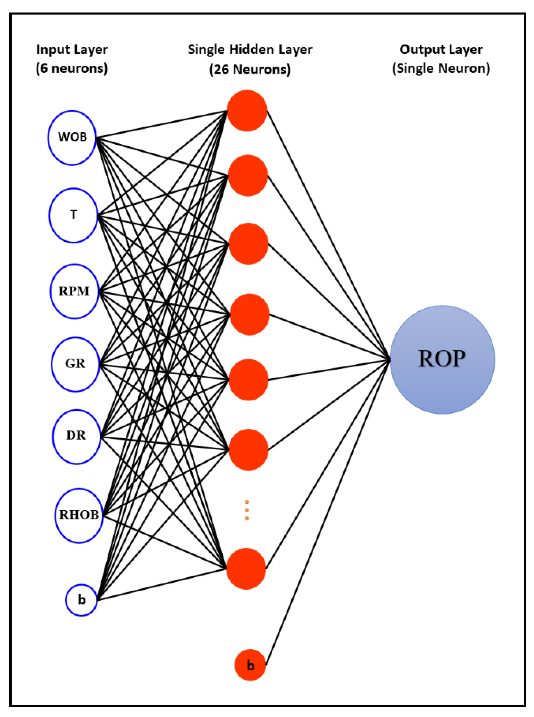
2.2. Training the ANN Model

The dataset collected from Well-A (3531 data points) was used to build the ANN model, with 85% of this data randomly selected to train the ANN model and 15% used for testing the trained model. These percentages were selected based on the optimization process, as discussed later in this section.
The training dataset was first analyzed statistically to determine the ranges for the different parameters used to develop the ANN model; the results of this analysis are summarized in Table 1. As indicated in Table 1, RPM ranged from 59.8 to 132, T was between 3.06 and 7.81 kft.lbf, WOB was from 5.55 to 24.3 klbf, GR was between 8.80 and 69.5 API, RHOB ranged from 2.13 to 3.02 g/cm3, and ROP was from 6.53 to 53.2 ft/hr. The ranges of the training data, as summarized in Table 1 were very important and needed to be considered when predicting ROP. To ensure high accuracy during ROP predictions, the new input dataset used for the ROP estimation had the same range as the training data.
Figure 1 compares the relative importance of the input parameters used to train the ANN model. The inputs used in this study were selected based on their relative importance to the ROP. As shown in Figure 1, the T and WOB had good correlation coefficients with the ROP, i.e., 0.67 and 0.61, respectively. RPM and DR had acceptable correlations with the ROP. Although GR and RHOB had low correlation coefficients of 0.07 and 0.13, respectively, with the ROP, they were considered as inputs in this study because they both directly affected the ROP. Changes in GR and RHOB gave indications about the change in the lithology, which led to a change in ROP. The use of GR to improve ROP predictability for horizontal wells was suggested previously by Mantha and Samuel [42].
After preprocessing the training data, the SaDE algorithm was applied to optimize the ANN model to select a combination of ANN design parameters to predict ROP with the minimum AAPE and highest correlation coefficient (R) and coefficient of determination (R2).
Different design parameters of the ANN model were studied during the optimization process, including the percentage of the training and testing data, training function, transfer function, number of hidden layers, and the number of neurons associated with every hidden layer. The effect of using 5% to 95% of the data collected from Well-A for training was evaluated during model optimization. The predictability of different training functions, such as Levenberg–Marquardt backpropagation, BFGS (Broyden–Fletcher–Goldfarb–Shanno) Quasi-Newton backpropagation (trainbfg), conjugate gradient, Bayesian regularization backpropagation, gradient descent with adaptive learning rate backpropagation, and gradient descent with momentum backpropagation, was evaluated. The effects on training accuracy of transfer functions log-sigmoid (logsig), tan-sigmoid, and pure-line were also evaluated. The use of 1–3 hidden layers, with 5–30 neurons per layer, was also studied.
The optimization process was conducted using SaDE in MATLAB®. Based on the results of the optimization process, the use of the trainbfg function to train the ANN model and the logsig transfer function with a single hidden layer with 26 neurons, as listed in Table 2, optimized the ANN model for ROP prediction. The structure of the suggested ANN model for ROP prediction is shown in Figure 2, which shows that the ANN model had an input layer with 6 neurons (one neuron for every input variable), a single layer with 26 neurons, and one output layer with a single output neuron (i.e., ROP).
An empirical correlation based on the weights and biases of the optimized ANN model with the design parameters, as listed in Table 2, was then developed. In this step, the optimized ANN model was converted from a black box to a white box for easy use and to program the developed correlation for future use.

2.3. Testing and Validation of the Developed ANN-Based Correlation

After developing the empirical correlation, the remaining 531 data points of Well-A, which represented 15% of the Well-A data, were used to test the developed ANN-based correlation, which was then validated using the 3600 unseen data points collected from Well-B. Before testing or validating the developed correlation, the ranges of the testing and validation datasets were investigated and confirmed to fall within the range of the data used to train the ANN model, which is summarized in Table 1. This step was very important to ensure that the ROP was accurately predicted. The predictability of the developed ANN-based correlation for ROP for the validation data was compared with the predictability of four commonly used empirical correlations for ROP estimation, namely, Maurer’s [11], Bingham’s [12], Bourgoyne and Young’s [13], and Osgouei’s [6] correlations, as presented earlier in Equations (1)–(3), and (11).

2.4. Evaluation Criteria

Four metrics were considered in this study to evaluate the predictive power of the developed ANN model and ANN-based empirical correlation for ROP estimation, namely, AAPE, R2, R, and a visualization check of the match between the actual and the predicted ROP. These metrics were considered sufficient to evaluate the predictability of the ROP for training, testing, and validation datasets.

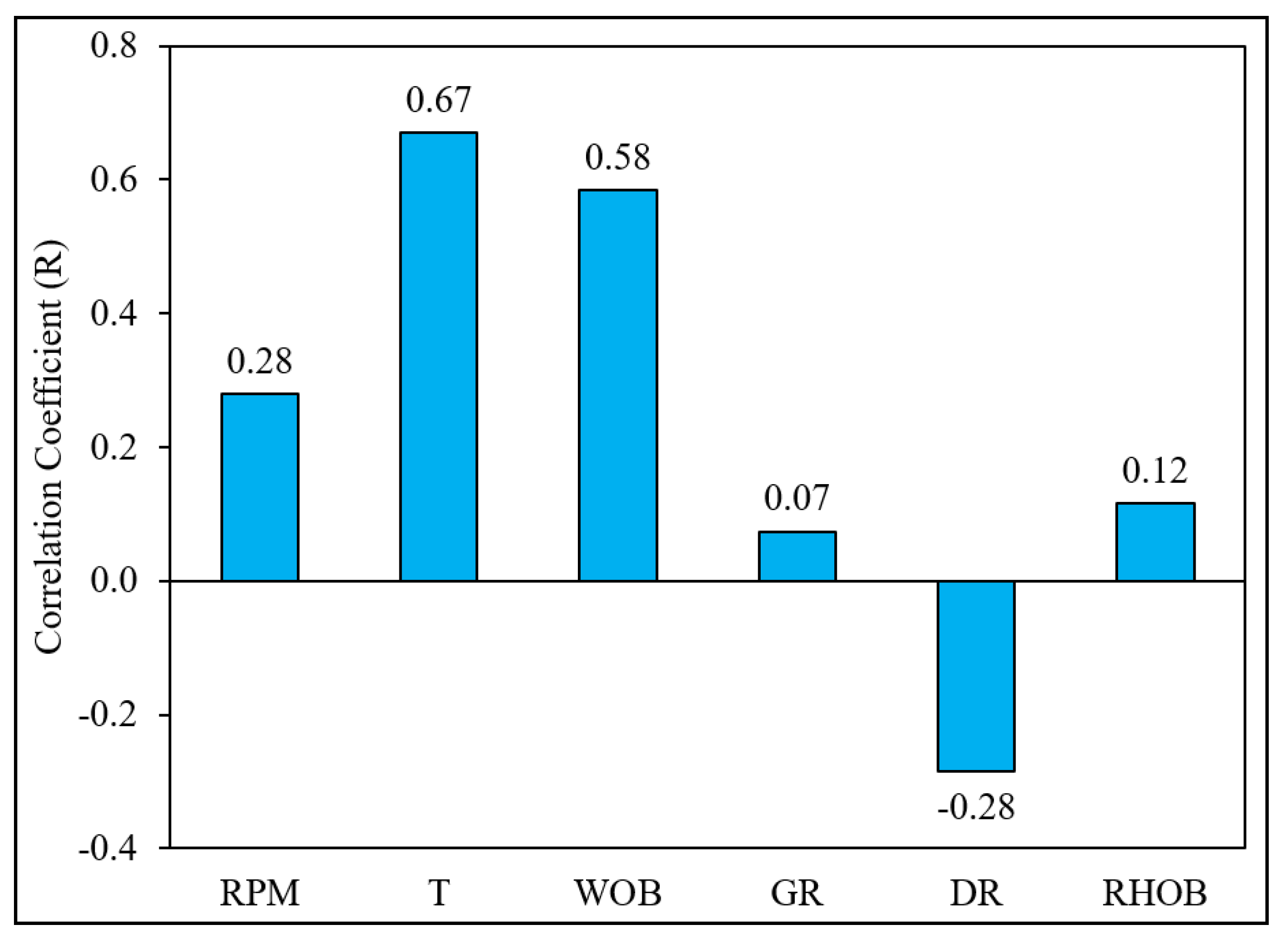
3. Results and Discussion

3.1. Training the ANN model

The ANN model developed in this study was trained using 3000 datasets, including RPM, T, WOB, GR, DR, and RHOB as inputs to predict the ROP as an output. The training data was randomly selected from Well-A data and represented 85% of the total data available from Well-A. The SaDE algorithm was used to optimize the ANN model to predict the ROP; Table 2 summarizes the optimum ANN parameters for ROP estimation.
The training data and their corresponding actual and ANN predicted ROP values are summarized in Figure 3 as a function of well depth. The results in Figure 3 show that the ANN model predicted the ROP for the training dataset of Well-A with a low AAPE of 5.12% and a considerably high R of 0.960, confirming a good match between the actual and predicted ROP curves, indicating high accuracy of the developed ANN model in estimating ROP.
Figure 4 shows a cross-plot of the actual ROP versus the predicted ROP for the training dataset (85% of Well-A data), indicating high accuracy of the ANN model in estimating the ROP with an R2 of 0.921.

3.2. Developing the ANN-Based Correlation

The proposed ANN-based empirical model was given by Equations (20)–(27).
R O P n =   i = 1 N w 2 i 1 1 + e ( w 1 i , 1 R P M n + w 1 i , 2 T n + w 1 i , 3 W O B n + w 1 i , 4 G R n + w 1 i , 5 D R n + w 1 i , 6 R H O B n + b 1 i ) + b 2
where ROPn is the normalized ROP, N represents the number of neurons in first hidden layer (26 neurons), i denotes the index of each neuron in the hidden layer, as shown in Table 3, w1i is the weight associated with input and hidden layers for each input parameter, b1i denotes the biases associated with the input and training layers, w2i is the weight associated with the hidden and output layers, RPMn, Tn, WOBn, GRn, DRn, and RHOBn represent the normalized RPM, T, WOB, GR, DR, and RHOB, respectively, and b2 is the bias associated with the hidden and output layers, which was 0.248 in this case. All weights and biases needed for Equation (20) are listed in Table 3.
The normalized input parameters in Equation (20) were calculated using Equations (21)–(26).
R P M n = 0.0277 ( R P M 59.76 ) 1
T n = 0.421 ( T O R Q U E 3.0633 ) 1
W O B n = 0.1066 ( W O B 5.5520 ) 1
G R n = 0.0329 ( G R 8.8038 ) 1
D R n = 0.0021 ( D R 0.6449 ) 1
R H O B n = 2.2589 ( R H O B 2.1345 ) 1
The value of ROPn, as calculated by Equation (20), was the normalized ROP, which was converted to the real ROP using Equation (27).
R O P =   R O P n + 1 0.0429 + 6.5345

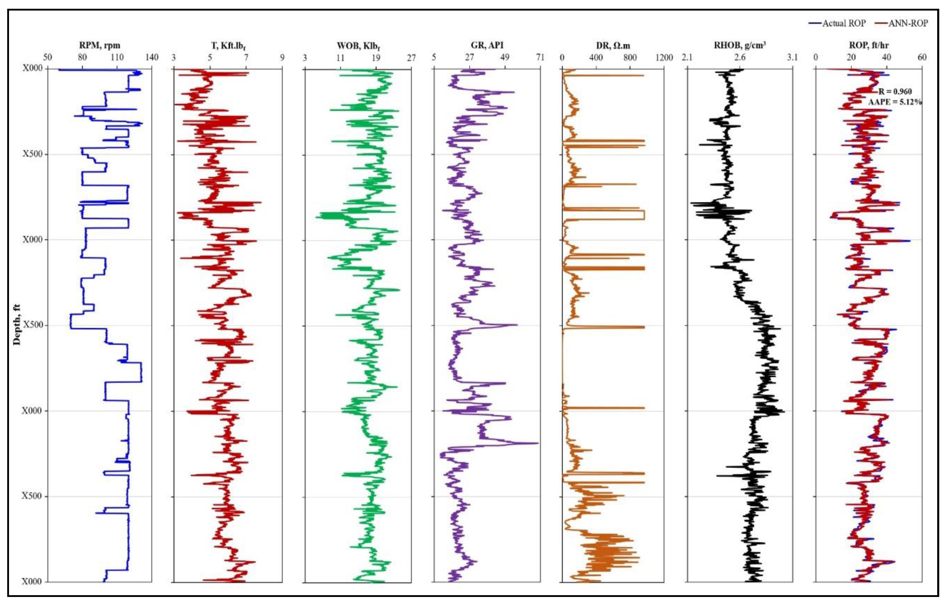
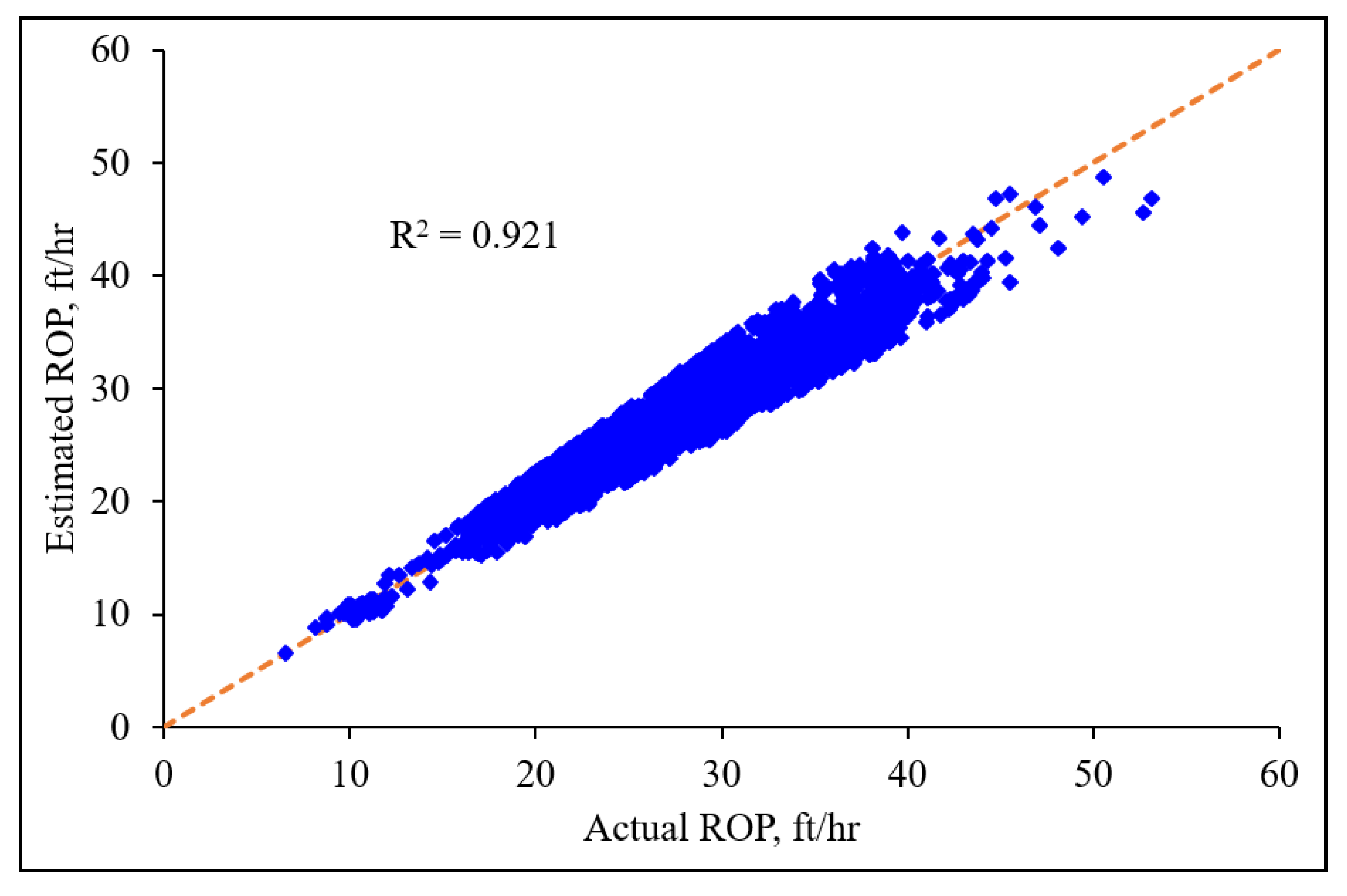
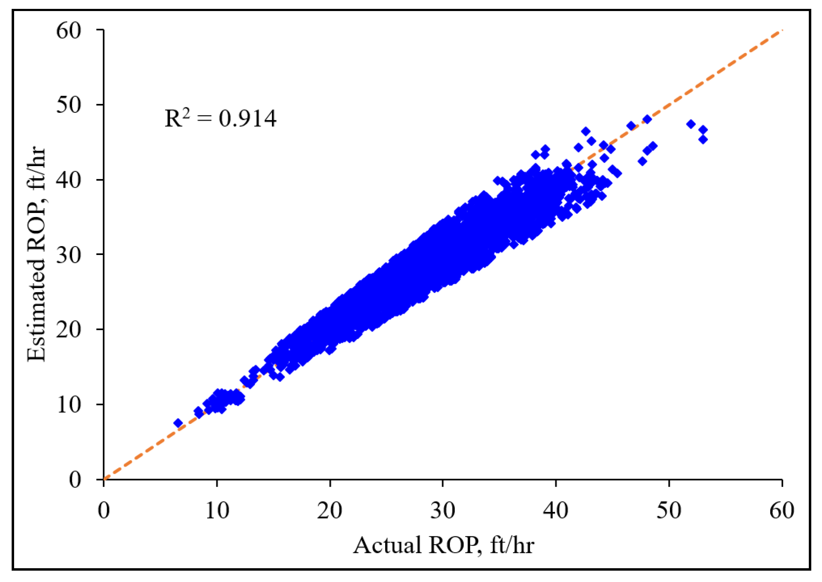
3.3. Testing the Developed ANN-Based Correlation

The ANN-based model developed in this study, as summarized in Equations (20)–(27), was then tested using the remaining unseen 15% of the data of Well-A. Figure 5 compares the actual ROP with the ROP values estimated using the ANN-based empirical equations (Equations (20)–(27)) for the Well-A test dataset. As indicated in Figure 5, the ANN-based empirical equations were able to predict the ROP with high accuracy, as indicated by the low AAPE of 5.80% and the high R of 0.951. Figure 5 shows high accuracy. Also shows high accuracy of the ANN-based correlation, where there was a good match between the actual and predicted ROP curves.
Figure 6 compares the actual ROP with the predicted value using the ANN-based empirical correlation. As indicated in Figure 6, the ANN-based equation predicted the ROP for the test dataset (15% of the data of Well-A) with high accuracy in terms of the R2 (R2 = 0.905).

3.4. Validation of the Developed ANN-Based Empirical Correlation

The accuracy of the ANN-based empirical correlation predictions using Equations (20)–(27) was validated using another set of unseen data collected from Well-B. Figure 7 shows the input variables of RPM, T, WOB, GR, DR, and RHOB used to predict the ROP in Well-B, and also compares the ROP values predicted using the ANN-based correlation (Equations (20)–(27)) with the actual ROP. As indicated in Figure 7, the AAPE and R of the predicted ROP were 5.29% and 0.956, respectively. The low AAPE and high R of the predicted ROP indicated the high accuracy of the developed ANN-based correlation. A visual check of the actual and ANN-based ROP values in Figure 7 also indicated a good match between the two curves (i.e., the actual ROP and the ANN-ROP), thereby confirming high accuracy of the ANN-based correlation.
Figure 8 compares the actual ROP with the predicted value using the ANN-based empirical correlations, as summarized in Equations (20)–(27) for the validation dataset (3600 data points collected from Well-B). As indicated in Figure 8, the ANN-based equation predicted the ROP for the validation dataset with a relatively high R2 of 0.914, indicating high accuracy of the developed ANN-based correlation.

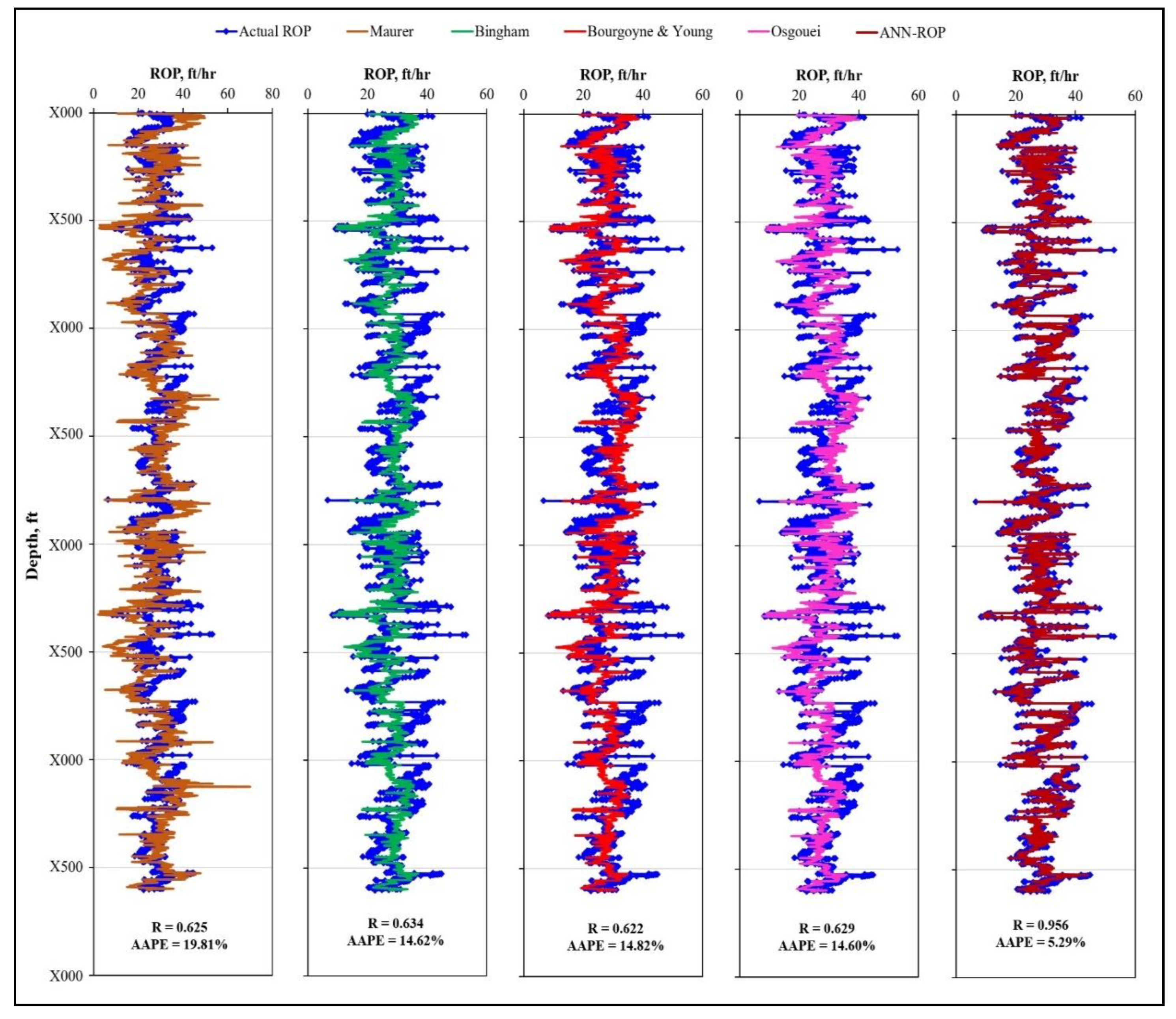
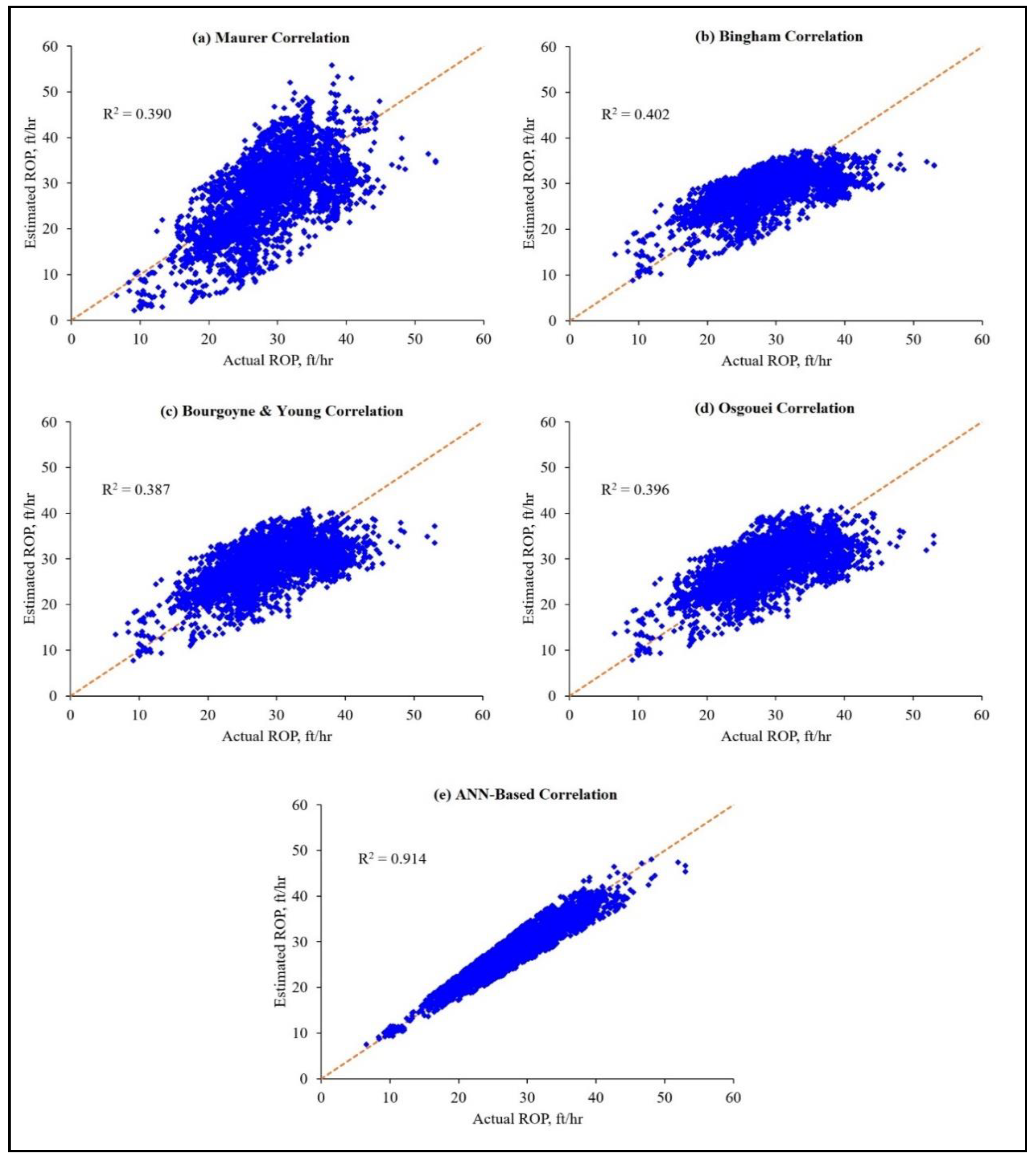
3.5. Comparison of the Predictability of the Developed ANN-Based Empirical Correlation with Available Correlations

In this section of the study, the accuracy of four currently available empirical equations for ROP estimation, namely, Maurer’s, Bingham’s, Bourgoyne and Young’s, and Osgouei’s correlations, was compared to the accuracy of the developed ANN-based empirical correlation in Equations (20)–(27). As shown in Figure 9, Maurer’s correlation was the least accurate correlation in terms of ROP estimation according to the validation data, with the highest AAPE of 19.81% and a very low R of 0.625. Bourgoyne and Young’s correlation predicted the ROP with an AAPE of 14.82% and an R of 0.622, while the ROP predicted by Bingham’s correlation had AAPE and R values of 14.62% and 0.634, respectively. Osgouei’s correlation was the best empirical correlation of the available correlations in terms of predicting the ROP, with the lowest AAPE of 14.60% and an R of 0.629.
The developed empirical correlation based on ANN, which was summarized in Equations (20)–(27), outperformed all available correlations in predicting ROP for the Well-B validation data, as indicated by the very low AAPE and very high R values of 5.29% and 0.956, respectively, as shown in Figure 9. Visual checking of the predicted ROP curves with the different correlations and the actual ROP shown in Figure 9 indicated an excellent match between the actual and ANN-based empirical correlation compared to all of the available correlations.
Figure 10 shows cross-plots comparing the actual ROP with the ROP values (3600 data points of Well-B) calculated using the different empirical correlations. As indicated in this figure, none of the available correlations accurately predicted the ROP, as indicated by the low R2 values between the actual and predicted ROPs. Maurer’s and Bourgoyne and Young’s correlations predicted the ROP with R2 values of only 0.390 and 0.387, respectively. Bingham’s and Osgouei’s correlations predicted the ROP with slightly higher R2 values of 0.402 and 0.396, respectively. The ANN-based correlation predicted the ROP with a very high R2 value of 0.914.
As shown in Figure 10a–d, the cross-plots of the actual and predicted ROP values using the previously developed correlations were highly scattered compared to the cross-plot for the ROP values predicted using the ANN (Figure 10e).

4. Conclusions

A new correlation to estimate ROP while drilling horizontal wells in carbonation formations was developed based on the extracted weights and biases of the trained and optimized ANN model. The ANN model was optimized using a self-adaptive differential evolution algorithm. The developed correlation estimated ROP as a function of the drilling parameters of the RPM, torque (T), and WOB, combined with conventional GR, DR, and RHOB well log data. The following observations were made:
  • The optimized ANN model predicted the ROP for the training dataset (3000 data points) with an AAPE of 5.12% and a correlation coefficient (R) of 0.960;
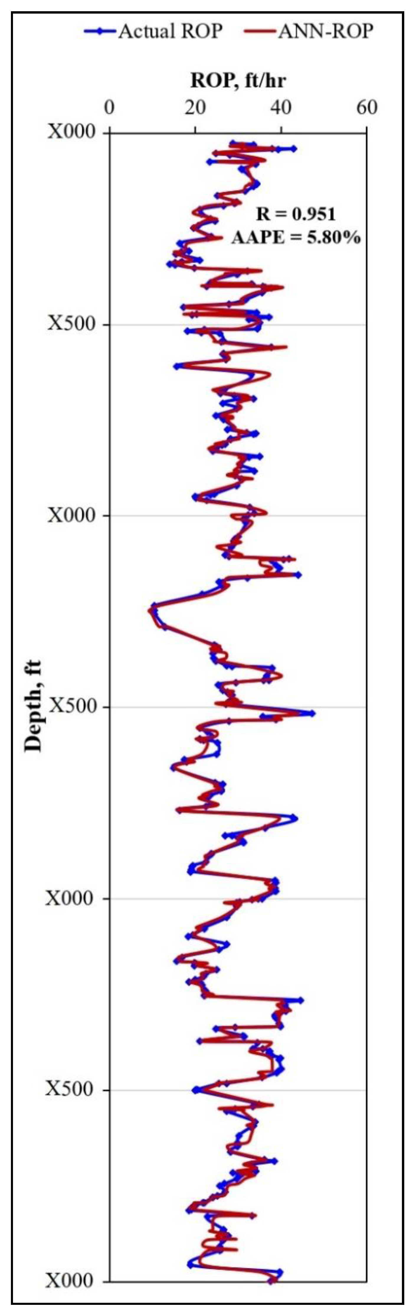
  • The developed correlation predicted the ROP for the testing dataset (531 data points) with AAPE and R values of 5.80% and 0.951, respectively;
  • The developed ROP correlation outperformed a recently developed empirical correlation for estimating ROP in directional wells (the Osgouei model), which predicted the ROP for the validation data with a high AAPE and a low R of 14.60% and 0.629, respectively;
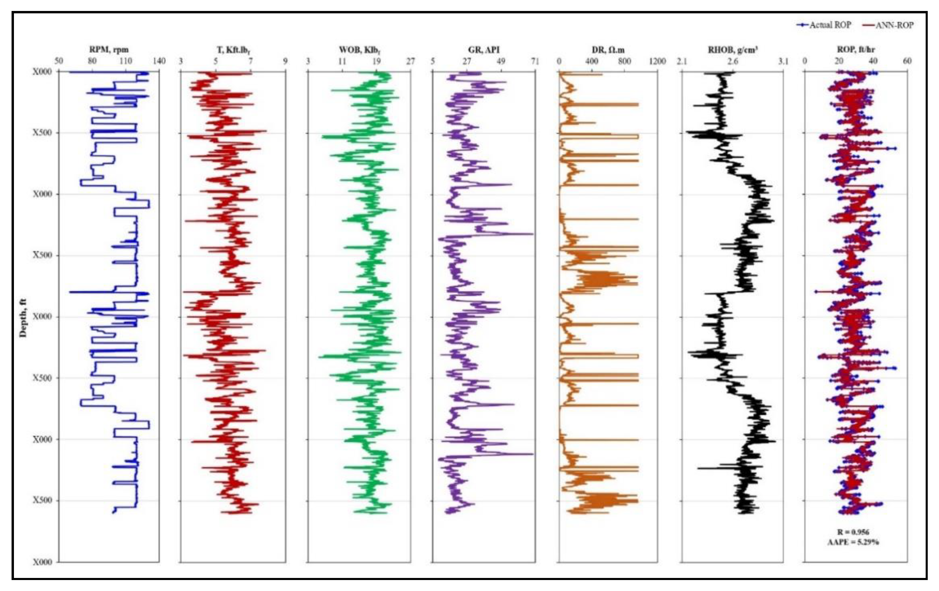
  • The developed correlation predicted ROP for the validation dataset of Well-B (3600 data points) with an AAPE of only 5.26% and a high R of 0.956.

Author Contributions

Conceptualization, S.E; data preparation, S.E., A.A.-A., and A.A.M.; model development, A.A.-A., and T.M.; results analysis, A.A.M.; writing—original draft preparation, A.A.M.; writing—review and editing, S.E., M.A., D.A.-S., and A.A.-Y.; supervision, S.E. All authors read and agreed to the published version of the manuscript.

Funding

This research was funded by [Saudi Aramco] grant number [CIPR2321].

Acknowledgments

Authors would like to acknowledge the College of Petroleum and Geoscience at King Fahd University of Petroleum and Minerals and Saudi Aramco for the support and permission to publish this work. We also acknowledge Saudi Aramco for funding this research under project number CIPR2321.

Conflicts of Interest

The authors declare no conflict of interest.

Appendix A

AAPEAverage Absolute Percentage Error
AIArtificial Intelligence
ANNArtificial Neural Network
DEDifferential Evolution
DRDeep Resistivity
ECDEquivalent Circulation Density
GPMPumping Rate
GRGamma Ray
logsiglog-sigmoid
MWMud Density
PVPlastic Viscosity
RCorrelation Coefficient
R2Coefficient of Determination
RHOBFormation Bulk Density
ROPRate of Penetration
RPMRotation Speed
SaDESelf-Adaptive Differential Evolution
SPPStandpipe Pressure
SVMSupport Vector Machine
TTorque
trainbfgBFGS Quasi-Newton Backpropagation
WOBWeight-on-Bit

References

  1. Lyons, W.C.; Plisga, G.J. Standard Handbook of Petroleum and Natural Gas. Engineering, 2nd ed.; Gulf Professional Publishing: Woburn, MA, USA, 2004; ISBN 10: 0750677856. [Google Scholar]
  2. Barbosa, L.F.F.M.; Nascimento, A.; Mathias, M.H.; de Carvalho, J.A., Jr. Machine learning methods applied to drilling rate of penetration prediction and optimization-A review. J. Pet. Sci. Eng. 2019, 183, 106332. [Google Scholar] [CrossRef]
  3. Hossain, M.E.; Al-Majed, A.A. Fundamentals of Sustainable Drilling Engineering, 1st ed.; Wiley-Scrivener: Austin, TX, USA, 2015; ISBN 10: 0470878177. [Google Scholar]
  4. Eren, T.; Ozbayoglu, M.E. Real time optimization of drilling parameters during drilling operations. In Proceedings of the SPE Oil and Gas India Conference and Exhibition, Mumbai, India, 20–22 January 2010. SPE-129126-MS. [Google Scholar] [CrossRef] [Green Version]
  5. Payette, G.S.; Spivey, B.J.; Wang, L.; Bailey, J.R.; Sanderson, D.; Kong, R.; Pawson, M.; Eddy, A. Real-time well-site based surveillance and optimization platform for drilling: Technology, basic workflows and field results. In Proceedings of the SPE/IADC Drilling Conference and Exhibition, The Hague, The Netherlands, 14–16 March 2017. SPE-184615-MS. [Google Scholar] [CrossRef]
  6. Osgouei, R.E. Rate of Penetration Estimation Model for Directional and Horizontal Wells. Master’s Thesis, Middle East Technical University, Ankara, Turkey, 2007. [Google Scholar]
  7. Soares, C.; Daigle, H.; Gray, K. Evaluation of PDC bit ROP models and the effect of rock strength on model coefficients. J. Nat. Gas Sci. Eng. 2016, 34, 1225–1236. [Google Scholar] [CrossRef]
  8. Soares, C.; Gray, K. Real-time predictive capabilities of analytical and machine learning rate of penetration (ROP) models. J. Pet. Sci. Eng. 2019, 172, 934–959. [Google Scholar] [CrossRef]
  9. Mitchell, R.F.; Miska, S.Z. Fundamentals of Drilling Engineering; Society of Petroleum Engineers: Richardson, TX, USA, 2011; ASIN: B01L0O8WJA. [Google Scholar]
  10. Hegde, C.; Daigle, H.; Millwater, H.; Gray, K. Analysis of Rate of Penetration (ROP) Prediction in Drilling Using Physics-Based and Data-Driven Models. J. Pet. Sci. Eng. 2017, 159, 295–306. [Google Scholar] [CrossRef]
  11. Maurer, W. The “perfect-cleaning” theory of rotary drilling. J. Pet. Technol. 1962, 14, 1270–1274. [Google Scholar] [CrossRef]
  12. Bingham, M.G. A New Approach to Interpreting Rock Drillability; Petroleum Publishing Co.: Tulsa, OK, USA, 1965. [Google Scholar]
  13. Bourgoyne, A.; Young, F.S. A multiple regression approach to optimal drilling and abnormal pressure detection. Soc. Pet. Eng. J. 1974, 14, 371–384. [Google Scholar] [CrossRef]
  14. Mahmoud, A.A.; Elzenary, M.; Elkatatny, S. New Hybrid Hole Cleaning Model for Vertical and Deviated Wells. J. Energy Resour. Technol. 2020, 142, 034501. [Google Scholar] [CrossRef]
  15. Hag Elsafi, S. Artificial Neural Networks (ANNs) for flood forecasting at Dongola Station in the River Nile, Sudan. Alex. Eng. J. 2014, 53, 655–662. [Google Scholar] [CrossRef]
  16. Babikir, H.A.; Abd Elaziz, M.; Elsheikh, A.H.; Showaib, E.A.; Elhadary, M.; Wu, D.; Liu, Y. Noise prediction of axial piston pump based on different valve materials using a modified artificial neural network model. Alex. Eng. J. 2019, 58, 1077–1087. [Google Scholar] [CrossRef]
  17. Nayak, S.C.; Misra, B.B.; Behera, H.S. Artificial chemical reaction optimization based neural net for virtual data position exploration for efficient financial time series forecasting. Ain Shams Eng. J. 2018, 9, 1731–1744. [Google Scholar] [CrossRef]
  18. Jana, G.C.; Swetapadma, A.; Pattnaik, P.K. Enhancing the performance of motor imagery classification to design a robust brain computer interface using feed forward back-propagation neural network. Ain Shams Eng. J. 2018, 9, 2871–2878. [Google Scholar] [CrossRef]
  19. Abdelwahed, M.F.; Mohamed, A.E.; Saleh, M.A. Solving the motion planning problem using learning experience through case-based reasoning and machine learning algorithms. Ain Shams Eng. J. 2019, in press. [Google Scholar] [CrossRef]
  20. Abd Elrehim, M.Z.; Eid, M.A.; Sayed, M.G. Structural optimization of concrete arch bridges using Genetic Algorithms. Ain Shams Eng. J. 2019, 10, 507–516. [Google Scholar] [CrossRef]
  21. Arehart, R.A. Drill-bit diagnosis with neural networks. SPE Comput. Appl. 1990, 2, 24–28. [Google Scholar] [CrossRef]
  22. Abdelgawad, K.; Elkatatny, S.; Moussa, T.; Mahmoud, M.; Patil, S. Real Time Determination of Rheological Properties of Spud Drilling Fluids Using a Hybrid Artificial Intelligence Technique. J. Energy Resour. Technol. 2018. [Google Scholar] [CrossRef]
  23. Elkatatny, S.M. Real Time Prediction of Rheological Parameters of KCl Water-Based Drilling Fluid Using Artificial Neural Networks. Arab. J. Sci. Eng. 2017, 42, 1655–1665. [Google Scholar] [CrossRef]
  24. Ren, X.; Hou, J.; Song, S.; Liu, Y.; Chen, D.; Wang, X.; Dou, L. Lithology identification using well logs: A method by integrating artificial neural networks and sedimentary patterns. J. Pet. Sci. Eng. 2019, 182, 106336. [Google Scholar] [CrossRef]
  25. Mahmoud, A.A.; Elkatatny, S.; Ali, A.; Abouelresh, M.; Abdulraheem, A. Evaluation of the Total Organic Carbon (TOC) Using Different Artificial Intelligence Techniques. Sustainability 2019, 11, 5643. [Google Scholar] [CrossRef] [Green Version]
  26. Mahmoud, A.A.; Elkatatny, S.; Abdulraheem, A.; Mahmoud, M.; Ibrahim, O.; Ali, A. New Technique to Determine the Total Organic Carbon Based on Well Logs Using Artificial Neural Network (White Box). In Proceedings of the 2017 SPE Kingdom of Saudi Arabia Annual Technical Symposium and Exhibition, Dammam, Saudi Arabia, 24–27 April 2017. SPE-188016-MS. [Google Scholar] [CrossRef]
  27. Mahmoud, A.A.; Elkatatny, S.; Ali, A.; Abouelresh, M.; Abdulraheem, A. New Robust Model to Evaluate the Total Organic Carbon Using Fuzzy Logic. In Proceedings of the SPE Kuwait Oil & Gas Show and Conference, Mishref, Kuwait, 13–16 October 2019. SPE-198130-MS. [Google Scholar] [CrossRef]
  28. Mahmoud, A.A.; Elkatatny, S.; Mahmoud, M.; Abouelresh, M.; Abdulraheem, A.; Ali, A. Determination of the total organic carbon (TOC) based on conventional well logs using artificial neural network. Int. J. Coal Geol. 2017, 179, 72–80. [Google Scholar] [CrossRef]
  29. Mahmoud, A.A.; Elkatatny, S.; Abouelresh, M.; Abdulraheem, A.; Ali, A. Estimation of the Total Organic Carbon Using Functional Neural Networks and Support Vector Machine. In Proceedings of the 12th International Petroleum Technology Conference and Exhibition, Dhahran, Saudi Arabia, 13–15 January 2020. IPTC-19659-MS. [Google Scholar] [CrossRef]
  30. Mahmoud, A.A.; Elkatatny, S.; Chen, W.; Abdulraheem, A. Estimation of Oil Recovery Factor for Water Drive Sandy Reservoirs through Applications of Artificial Intelligence. Energies 2019, 12, 3671. [Google Scholar] [CrossRef] [Green Version]
  31. Mahmoud, A.A.; Elkatatny, S.; Abdulraheem, A.; Mahmoud, M. Application of Artificial Intelligence Techniques in Estimating Oil Recovery Factor for Water Drive Sandy Reservoirs. In Proceedings of the 2017 SPE Kuwait Oil & Gas Show and Conference, Kuwait City, Kuwait, 15–18 October 2017. SPE-187621-MS. [Google Scholar] [CrossRef]
  32. Ahmed, A.S.; Mahmoud, A.A.; Elkatatny, S. Fracture Pressure Prediction Using Radial Basis Function. In Proceedings of the AADE National Technical Conference and Exhibition, Denver, CO, USA, 9–10 April 2019. AADE-19-NTCE-061. [Google Scholar]
  33. Ahmed, A.S.; Mahmoud, A.A.; Elkatatny, S.; Mahmoud, M.; Abdulraheem, A. Prediction of Pore and Fracture Pressures Using Support Vector Machine. In Proceedings of the 2019 International Petroleum Technology Conference, Beijing, China, 26–28 March 2019. IPTC-19523-MS. [Google Scholar] [CrossRef]
  34. Mahmoud, A.A.; Elkatatny, S.; Ali, A.; Moussa, T. Estimation of Static Young’s Modulus for Sandstone Formation Using Artificial Neural Networks. Energies 2019, 12, 2125. [Google Scholar] [CrossRef] [Green Version]
  35. Mahmoud, A.A.; Elkatatny, S.; Ali, A.; Moussa, T. A Self-adaptive Artificial Neural Network Technique to Estimate Static Young’s Modulus Based on Well Logs. In Proceedings of the Oman Petroleum & Energy Show, Muscat, Oman, 9–11 March 2020. SPE-200139-MS. [Google Scholar] [CrossRef]
  36. Elkatatny, S.; Tariq, Z.; Mahmoud, M.; Abdulraheem, A.; Mohamed, I. An integrated approach for estimating static Young’s modulus using artificial intelligence tools. Neural Comput. Appl. 2019, 31, 4123. [Google Scholar] [CrossRef]
  37. Elkatatny, S.; Tariq, Z.; Mahmoud, M.; Abdulraheem, A. New insights into porosity determination using artificial intelligence techniques for carbonate reservoirs. Petroleum 2018, 4, 408–418. [Google Scholar] [CrossRef]
  38. Elkatatny, S.; Aloosh, R.; Tariq, Z.; Mahmoud, M.; Abdulraheem, A. Development of a New Correlation for Bubble Point Pressure in Oil Reservoirs using Artificial Intelligence Technique. In Proceedings of the SPE Kingdom of Saudi Arabia Annual Technical Symposium and Exhibition, Dammam, Saudi Arabia, 24–27 April 2017. [Google Scholar] [CrossRef]
  39. Elkatatny, S.; Al-AbdulJabbar, A.; Mahmoud, A.A. New Robust Model to Estimate the Formation Tops in Real-Time Using Artificial Neural Networks (ANN). Petrophysics 2019, 60, 825–837. [Google Scholar] [CrossRef]
  40. Bilgesu, H.; Tetrick, L.; Altmis, U.; Mohaghegh, S.; Ameri, S. A new approach for the prediction of rate of penetration (ROP) values. In Proceedings of the SPE Eastern Regional Meeting, Lexington, Kentucky, 22–24 October 1997. SPE-39231-MS. [Google Scholar] [CrossRef]
  41. Amar, K.; Ibrahim, A. Rate of penetration prediction and optimization using advances in artificial neural networks, a comparative study. In Proceedings of the 4th International Joint Conference on Computational Intelligence, Barcelona, Spain, 5–7 October 2012; pp. 647–652. [Google Scholar] [CrossRef] [Green Version]
  42. Mantha, B.; Samuel, R. ROP Optimization Using Artificial Intelligence Techniques with Statistical Regression Coupling. In Proceedings of the SPE Annual Technical Conference and Exhibition, Dubai, UAE, 26–28 September 2016. SPE-181382-MS. [Google Scholar] [CrossRef]
  43. Elkatatny, S. New Approach to Optimize the Rate of Penetration Using Artificial Neural Network. Arab. J. Sci. Eng. 2018, 43, 6297–6304. [Google Scholar] [CrossRef]
  44. Ahmed, A.S.; Salaheldin, E.; Abdulraheem, A.; Mahmoud, M.; Ali, A.Z.; Mohamed, I.M. Prediction of Rate of Penetration of Deep and Tight Formation Using Support Vector Machine. In Proceedings of the SPE Kingdom of Saudi Arabia Annual Technical Symposium and Exhibition, Dammam, Saudi Arabia, 23–26 April 2018. SPE-192316-MS. [Google Scholar] [CrossRef]
  45. Monjezi, M.; Dehghani, H. Evaluation of effect of blasting pattern parameters on back break using neural networks. Int. J. Rock Mech. Min. Sci. 2008, 45, 1446–1453. [Google Scholar] [CrossRef]
  46. Angelini, E.; Ludovici, A. CDS Evaluation Model with Neural Networks. J. Serv. Sci. Manag. 2009, 2, 15. [Google Scholar] [CrossRef] [Green Version]
  47. Gurney, K. An Introduction to Neural Networks; UCL Press Limited: London, UK, 1997; ISBN 0-203-45151-1. [Google Scholar]
  48. Omran, M.G.H.; Salman, A.; Engelbrecht, A.P. Self-adaptive Differential Evolution. In Computational Intelligence and Security; CIS 2005; Lecture Notes in Computer Science; Hao, Y., Liu, J., Wang, Y., Cheung, Y.-M., Yin, H., Jiao, L., Ma, J., Eds.; Springer: Berlin/Heidelberg, Germany, 2005; Volume 3801. [Google Scholar]
  49. Al-Anazi, A.F.; Gates, I.D. A support vector machine algorithm to classify lithofacies and model permeability in heterogeneous reservoirs. Eng. Geol. 2010, 114, 267–277. [Google Scholar] [CrossRef]
Figure 1. The relative importance of the input parameters for the training dataset.
Sustainability 12 01376 g001
Figure 2. The suggested artificial neural network (ANN) model for rate of penetration (ROP) prediction. The model had an input layer with 6 neurons for the 6 inputs, a single (hidden) training layer with 26 neurons, and one output layer with a single neuron as the output ROP. The letter b denotes the biases nodes.
Sustainability 12 01376 g002
Figure 3. From left to right, RPM, T, WOB, GR, DR, RHOB, and their corresponding actual and ANN-derived ROP for the training dataset (Well-A). The letter “X” in the depth’s axis was used to hide the exact depth, where “X” is a value from 1 to 9.
Sustainability 12 01376 g003
Figure 4. Cross-plot of the actual and predicted ROP values of the training dataset (3000 data points, Well-A).
Sustainability 12 01376 g004
Figure 5. The actual and ANN-derived ROP for the training dataset (Well-A). The letter “X” in the depth’s axis was used to hide the exact depth, where “X” is a value from 1 to 9.
Sustainability 12 01376 g005
Figure 6. Cross-plot of the actual and predicted ROP of the testing dataset (531 data points, Well-A).
Sustainability 12 01376 g006
Figure 7. From left to right, RPM, T, WOB, GR, DR, RHOB, and their corresponding actual and ANN-derived ROP values for the validation dataset (Well-B). The letter “X” in the depth’s axis was used to hide the exact depth, where “X” is a value from 1 to 9.
Sustainability 12 01376 g007
Figure 8. Cross-plot of the actual and predicted ROP values of the validation dataset (3600 data points, Well-B).
Sustainability 12 01376 g008
Figure 9. Comparison of the predictability of Maurer’s, Bingham’s, Bourgoyne and Young’s, Osgouei;s, and ANN-based correlations for ROP with the actual ROP according to the validation dataset.
Sustainability 12 01376 g009
Figure 10. Cross-plots of the actual and predicted ROP using (a) Maurer’s, (b) Bingham’s, (c) Bourgoyne and Young’s, (d) Osgouei’s, and (e) ANN-based correlations for the validation dataset (3600 data points, Well-B).
Sustainability 12 01376 g010
Table 1. The statistical parameters for the training dataset (85% of the data collected from Well-A).
Statistical ParametersRPM (rpm)T (kft.lbf)WOB (klbf)GR (API)DR (Ω.m)RHOB (g/cm3)ROP (ft/hr)
Minimum59.83.065.558.800.642.1359.8
Maximum1327.8124.369.59653.02132
Range72.24.7518.860.7963.90.8972.2
Standard Deviation17.50.752.648.5212.40.1617.5
Sample Variance3060.576.9972.9451140.02306
Kurtosis−1.140.161.551.966.09−0.87−1.14
Skewness−0.49−0.44−0.941.272.49−0.10−0.49
Table 2. Combination of the optimum ANN design parameters for ROP prediction.
ParameterValue
Training functiontrainbfg
Transfer functionlogsig
Number of hidden layers1
Number of neurons26
Table 3. Weights and biases for the first hidden layer of the ANN-based ROP model.
iw1i,1w1i,2w1i,3w1i,4w1i,5w1i,6b1iw2i
10.472−1.8693.127−1.3120.232−0.6216.4310.190
2−0.778−3.4541.8876.725−2.769−6.941−5.566−0.299
33.037−4.214−2.902−5.9271.752−0.969−4.7330.396
43.2792.073−4.9442.953−0.8966.679−5.680−0.654
5−1.1670.0341.637−4.192−0.988−3.3952.298−1.056
6−5.6140.971−4.185−2.940−0.1652.0193.5220.418
74.7121.8572.1613.803−1.979−0.936−3.0410.859
8−0.7950.1830.660−4.797−13.8421.330−14.488−0.945
93.732−4.144−3.459−1.0633.321−3.952−1.752−0.451
100.502−10.5245.8011.869−0.852−6.240−3.8570.294
11−0.317−5.3186.5443.2101.3600.4611.090−0.326
124.2120.7730.5921.9581.4702.034−0.118−0.388
132.9100.4333.3940.904−1.5100.177−0.7560.195
14−3.365−6.367−1.4623.218−5.9204.702−1.6460.416
15−2.4233.3260.483−3.764−3.841−4.8810.170−0.324
162.1905.4450.414−2.5460.930−2.493−1.0450.704
17−1.4432.0338.5484.1603.5509.202−0.1890.176
181.699−0.890−0.025−0.947−2.3173.959−0.119−0.379
19−2.2093.899−4.020−7.4171.5321.539−2.0220.738
20−1.2402.891−3.411−8.7621.5540.939−3.210−0.762
213.398−3.788−4.6021.518−1.2390.043−0.422−0.048
221.904−1.2896.963−1.6610.961−3.726−4.5470.378
23−3.9851.949−2.2661.4580.6862.434−4.530−1.069
24−0.462−1.8790.0583.5651.033−2.105−4.4230.795
25−0.8040.0430.667−3.192−10.1841.230−11.4191.249
26−5.700−2.821−1.0451.7652.478−3.574−6.170−0.580

