Beware Thy Bias: Scaling Mobile Phone Data to Measure Traffic Intensities

Abstract

Mobile phone data are a novel data source to generate mobility information from Call Detail Records (CDRs). Although mobile phone data can provide us with valuable insights in human mobility, they often show a biased picture of the traveling population. This research, therefore, focuses on correcting for these biases and suggests a new method to scale mobile phone data to the true traveling population. Moreover, the scaled mobile phone data will be compared to roadside measurements at 100 different locations on Dutch highways. We infer vehicle trips from the mobile phone data and compare the scaled counts with roadside measurements. The results are evaluated for October 2015. The proposed scaling method shows very promising results with near identical vehicle counts from both data sources in terms of monthly, weekly, and hourly vehicle counts. This indicates the scaling method, in combination with mobile phone data, is able to correctly measure traffic intensities on highways, and thereby able to anticipate calibrated human mobility behaviour. Nevertheless, there are still some discrepancies—for one, during weekends—calling for more research. This paper serves researchers in the field of mobile phone data by providing a proven method to scale the sample to the population, a crucial step in creating unbiased mobility information.

1. Introduction

Samples are strongly influenced by the information present in the environment [1]. In practice this means that samples are practically never truly random, which leads to biases in resulting judgements [1]. Furthermore, humans often reason through heuristics explaining a simplified version of the world [2]. Although these simplifications are useful they can result in severe systematic errors [2]. To create an unbiased view of the population these biases have to be addressed and corrected for [1]. In this paper we, therefore, address and provide a method for correcting structural biases in mobile phone data, i.e., mobility data generated from Call Detail Records (CDRs) of mobile providers and scale it to the traveling population.

Mobile phone data is a hot topic in the field of human mobility studies. A vast amount of recent research has been performed that investigates the use of mobile phone data to gather better insights into behaviour, social networks and mobility patterns of the masses [3,4,5,6,7,8]. Mobile phone data is regarded a prime candidate to replace traditional mobility measurement techniques such as surveys and roadside measurements [9,10]. Mobile phone data can provide us with mobility information on unprecedented scale [10,11]. Where surveys provide a snapshot of the lives of a few thousand inhabitants, mobile phone data can provide 24/7 information on millions of people [9,10]. This new data source is already providing us with new and unique insights into human mobility [12,13].

Provided the increasing use of this new data source, making sure the results are unbiased also becomes more important. Studies that employ mobile phone data, however, generally pay little attention to the bias in mobile phone data while scaling the sample to the population. The latter is a must when comparing values on different scales. Scaling is in essence performed for the same purpose as calibrating in any other type of measurement device. To exemplify, mercury in a thermometer will expand when temperature increases. However, unless the thermometer is calibrated the only conclusion can be that it became warmer or colder. We do not know by how much temperature increased nor are we able compare with measurements of other thermometers.

Studies such as the one by Jiang, Ferreira and González [14] recognize this fact. Jiang et al., for one, scale the sample to the population based on the ratio of sample to population for different geographic areas. Cools, Moons and Wets [15] take a similar approach with the extension of removing users with few events, for whom they argue no trustworthy origins and destinations can be established. Iqbal et al. [16] built Origin Destination (OD) matrices from CDRs and calibrated their OD matrices using road side measurements. The disadvantage of calibration is having to rely on a second source of information limiting its use in practice, especially for areas where less information is available. In this study we will build upon the approaches by Jiang et al. and Coole et al. by also compensating for the bias in the sample, which requires only census data unlike the calibrations such as the one performed by Iqbal et al. [14,16].

In the present study we address a bias identified in the mobile phone data. The bias we identified is introduced by demographic discrepancies between the traveling population and the sample from which mobile phone data is created. The bias is due to a difference in mobile phone possession and travel behaviour across age groups [17]. To illustrate, young children have both less chance to own a mobile phone as well as a lower chance to make a trip greater than 10 km, especially during schooldays, compared to 30 to 40 year olds [17]. Without compensating for this sampling bias we would get a biased view of the population, where especially age groups that travel less are underrepresented. Thus, when employing mobile phone data to answer mobility questions one needs to adjust for the bias to prevent erroneous conclusions.

We present and evaluate a method to scale the sample in mobile phone data to the population. To validate our proposed scaling method we will estimate vehicles present on a multitude of Dutch highways and compare the outcomes to roadside measurements. The advantage of comparing to roadside measurements rather than Origins and Destinations (ODs) from surveys is that the roadside measurements generally produce unbiased and highly accurate traffic counts [18,19,20,21]. The main goal of this study is to provide a validated scaling method for mobile phone data that could be used in future studies to get an unbiased view of the population.

This paper is structured as follows. In the next section we discuss the study area and provide a description of the data used in this study. Next, we will elaborate upon the methodology used in this research. Here also our scaling method is presented. Then, the results are presented followed by a discussion of these results. Finally, the conclusions of this research are presented.

2. Materials and Methods

2.1. Study Area and Data Description

The data available for this study covers the Netherlands as a whole. The Netherlands currently has 17 million inhabitants and spans 41.526 square km [22]. The country is approximately 200 km wide and 300 km tall and shares borders with Germany and Belgium. In 2015 80% of the population had a mobile phone of which the vast majority are smartphones [23,24]. The latter is relevant as the more people connect to the network, e.g., for calling but also receiving e-mail and browsing the web, the more events are generated and thus the more data points we have per inhabitant. This trickles down to better mobile phone data.

In the following sections we will elaborate on the CDRs, census data, survey data, and roadside measurement data used in this study.

2.2. Call Detail Records & Cell Tower Network

CDRs are the basis of mobile phone data. These are records describing when a mobile phone connected to the network by sending or receiving voice, text, or other data via a provider’s network. The records consists of a time stamp, a cell code relating to a cell tower in the network and a one-way hashed id created from a mobile phone number. At the time of writing about 370 million CDRs are generated per day by 3 million subscribers.

The network of cell towers of the provider consists of approximately 50.000 unique cells covering every part of the country. Geographic characteristics of the cell towers, i.e., their location and their radius, angle, and orientation are also provided by the provider. These geographic properties in combination with the CDRs enable us to pinpoint people at a certain moment in time.

The data used in this study is from one mobile network provider and covers October 2015.

2.3. Census Data & Geographic Zones

Census data forms the basis of the scaling method we present in this research. As previously explained, there is a bias in the sample mobile phone data provides due to demographic discrepancies. Census data provides us with crucial information about the population that allows us to assess our sample in comparison to the true population. In the Netherlands the Central Bureau of Statistics (CBS) reports census data. Age distribution on four digit postal code level is acquired from the CBS.

Where roadside measurement data as used by Iqbal et al. [16] might not be available everywhere, census data nearly always is. In addition, census data is often gathered in task of the government and is hence typically freely available [25]. As the census data is widely available and often accurate, the scaling method, which mainly relies on this source of information, could be implemented not only in the Netherlands, but also in many other countries all over the world. This greatly benefits the generalizability and enhances the overall value of the proposed method.

2.4. Mobility Survey Data

In essence the mobile phone data measures the movement of mobile phones and thus the people carrying the devices rather than the vehicles on the road. For a fair comparison, a translation is required to go from people to vehicles.

To get a good estimate of the number of people per vehicle, survey data from 5 years of Onderzoek Verplaatsingen in Nederland (‘Research Movements in The Netherlands’; OViN) are used, starting at 2010 and ending at 2014. OViN is chosen as it is the largest free nationwide mobility survey in the Netherlands [26]. When combined, the surveys contain 97.432 trips that are comparable to those in the mobile phone data. To be able to compare the data, we only selected trips 10 km or longer as we are interested in trips on highways, which are often longer than 10 km. Furthermore, we only selected trips with average travel velocities below 145 km/h, deeming them unrealistic and untrustworthy. For both calculation the distance taken is the distance as the crow flies from the origin postal code to the destination postal code.

An overview of the distribution of trips greater than 10 km per mode of transportation is shown in

Table 1. Different modes of transportation, their prevalence on the Dutch roads and the chance of being a driver (source: OViN).

Means of Transportation	% of Trips	Chance of being a Driver
Bus (public transport)	4.93%	11%
Bus (private)	0.57%	11%
Camper	0.05%	50%
Car (driver)	43.67%	100%
Car (passenger)	17.09%	0%
Delivery van	0.52%	95%
Motor	0.44%	87%
Taxi	0.44%	50%
Freight truck	0.06%	100%
Other / not on highway	32.23%	-

. The two largest groups by a margin are car (driver) and car (passenger). The third largest group bus (public transport) accounts for nearly 5% of all trips. The chance of being a driver for this class (11%) and the class motor is extracted from literature on Dutch public transport [27]. Bus (private) is assumed to be similar to bus (public transport). All other classes combined including taxi and freight truck only account for just over 1% of all trips. The assigned chances of being a driver for these classes are based on personal experience. Given their low share amongst all trips, the possible impact of mistakes due to guess work is considered to be negligible.

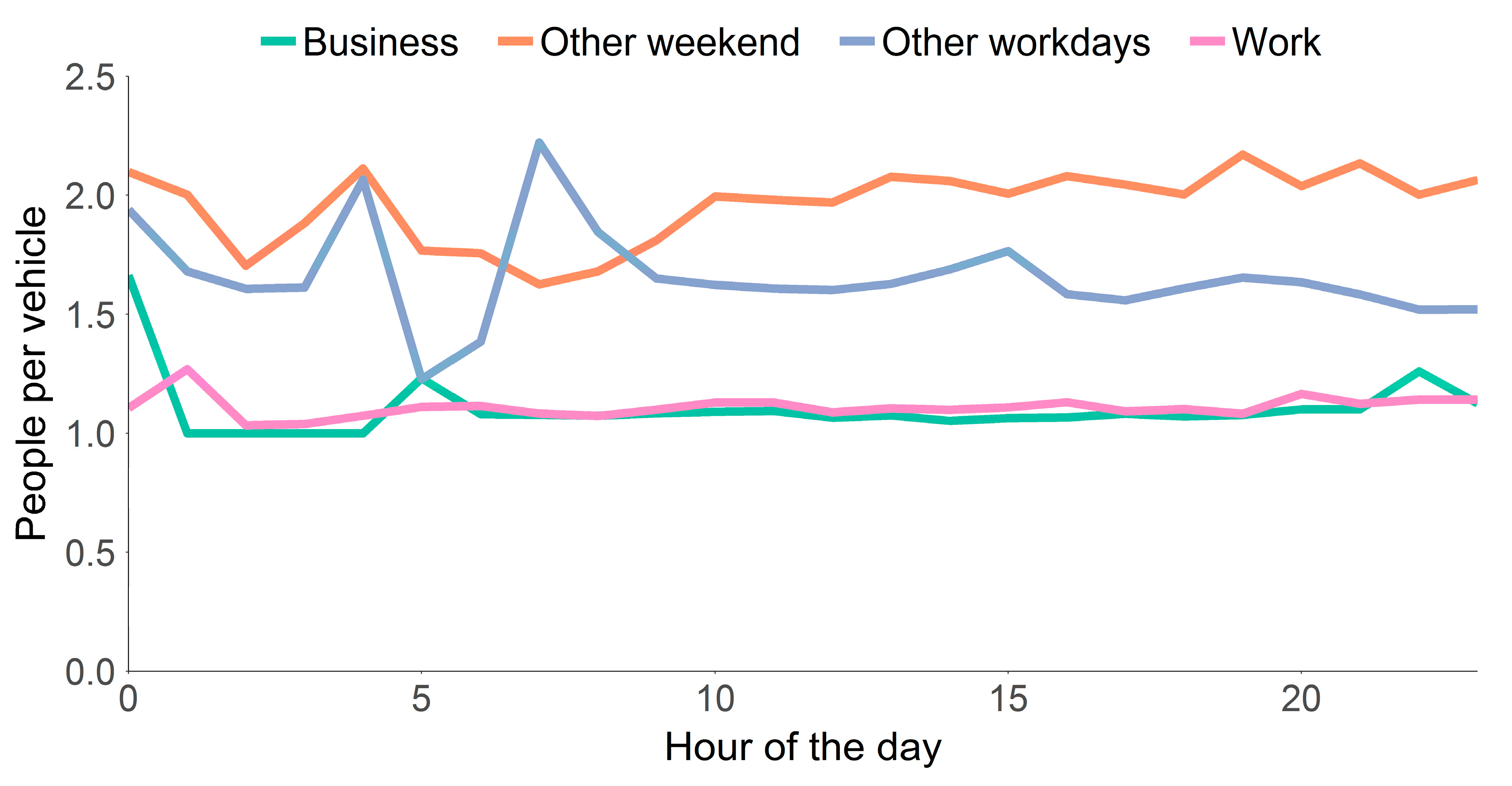
We find the motive of a trip, rather than hours of the day or day of the week, can provide very stable people per vehicle ratios. In Figure 1 the people per vehicle ratio, i.e., the inverse of the chance of being a driver, is depicted for each of the three motives, i.e., work, business and other, and hour of the day. As can be observed from Figure 1, the ratio people per vehicle is stable over the majority of the day. The unstable pattern in the early morning can be attributed to the small sample size in the early hours of the day. Note that we included the motive “other” twice, once for workdays and once for weekends. We did so because there is a clear difference in people per vehicle between the two day types for this motive. During the weekend there are generally more people per vehicle for non-work and business related activities than during workdays. The people per vehicle ratios applied are 2.02 for other weekend, 1.64 for other workdays, 1.08 for business, and 1.10 for work trips.

2.5. Mobile Phone Penetration

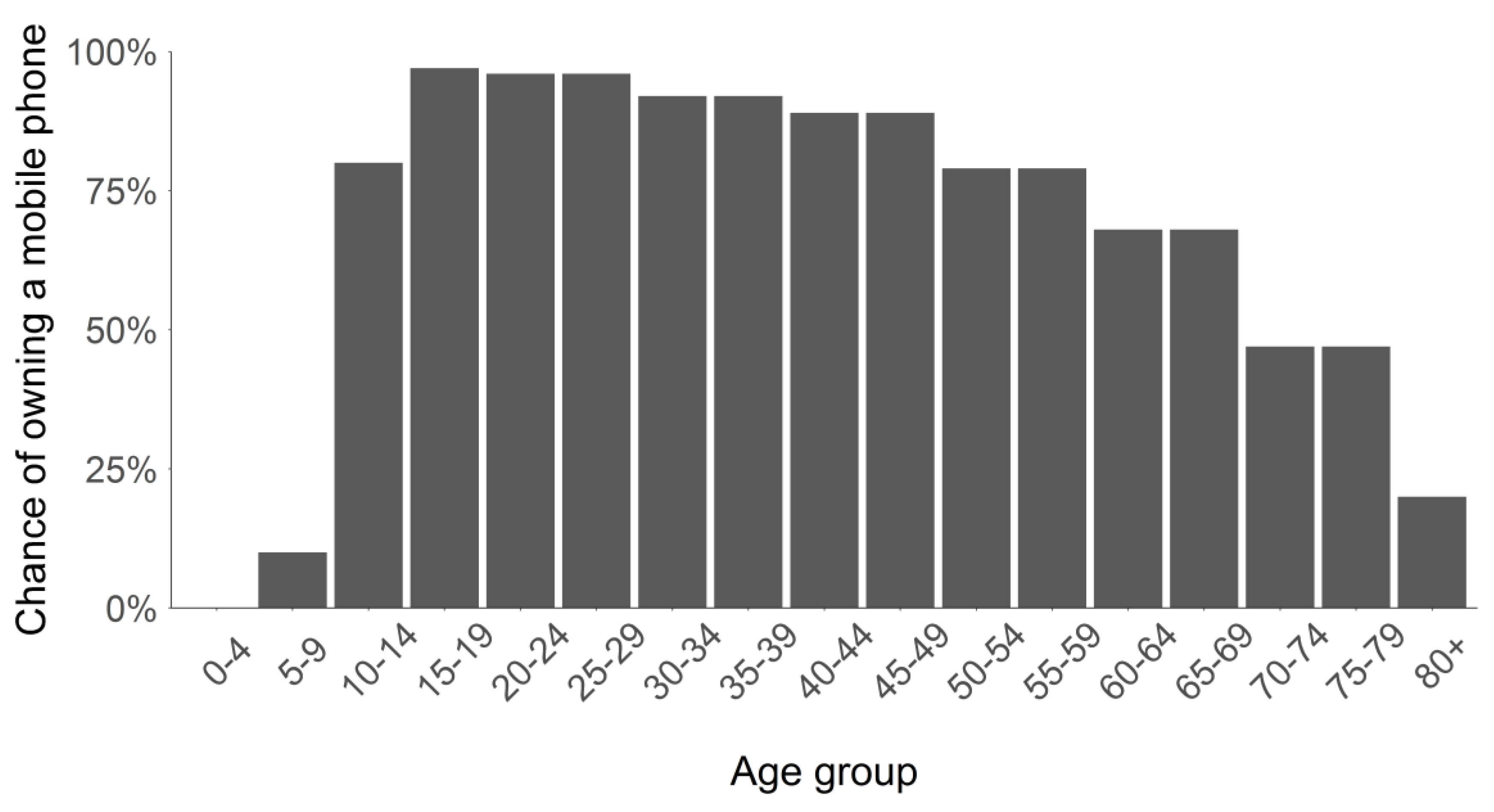
Figure 2 shows information about mobile phone penetration by age group, which was acquired via two sources. The first being Telecompaper [17], which contains the majority of the information used. Gaps, for people below age 12 and over 80, are filled by data from Offermans et al. [28]. The latter refers to a study by the Dutch statistical office, Statistics Netherlands (CBS), who assessed the representativeness of the sample of the mobile phone data used in this study, though with a two year gap. They also included information about the penetration of people having a smartphone at the telecom provider by age. This information, however, is not always available and hence we chose to use data from Telecompaper who provide a more nationwide assessment of smartphone penetration by age group. Moreover, they also provide information on a large variety of countries [17].

2.6. Roadside Measurement Data

In order to validate our scaling method we compared vehicles inferred from the mobile phone data with vehicles measured on the road. The number of vehicles measured on the road is obtained via road side measurements provided as open data by Nationale Databank Wegverkeersgegevens (‘National Database Traffic Data’; NDW). NDW is a governmental organization in the Netherlands that collects the measurement data from different parties such as Rijkswaterstaat. Most of the roadside measurements are collected by using an inductive-loop measurement devices placed on or in the road’s surface with a self-reported accuracy upwards of 99% [29,30]. An overview of the types of roadside measurement devices, the number of occurrences on the Dutch road network, and the mean self-reported accuracies of each type of device is shown in

Table 2. Roadside measurement devices in the Dutch road network (source: NDW).

Measurement Device	Counts	Accuracy
Inductive-loop vehicle detector	21.711	99%
Automatic Number-Plate Recognition	1.484	95%
Bluetooth	1.409	Unknown
Infrared	948	100%
Floating Car Data (from navigation systems)	24	Unknown

.

The information represented in Table 2 covers all measurement sites in the Netherlands, including information on the use of parking lots and gas station et cetera. Moreover, the measurements from these measurements sites contain predominantly raw data. For major roads Rijkswaterstaat cleaned the raw data by, for one, removing outliers. The algorithm processing the raw data is called Monibas, an algorithm that is proven to be highly accurate (Technical University Delft, 2006). The data processed by Monibas are also included in the raw data as a separate measurement sites. In total there are 13.693 measurement sites to which Monibas is applied, all of which employ raw data from inductive-loop vehicle detectors.

3. Research Approach

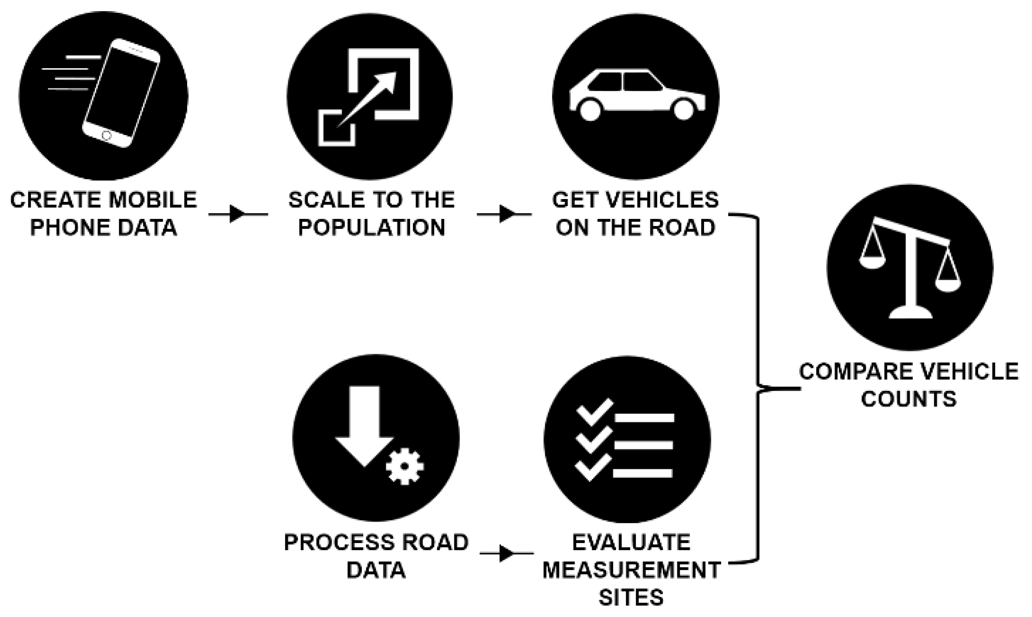
Our research methodology encompasses the steps taken to evaluate our scaling method. Part of the methodology is also the scaling method we present in this research. There are two main processes leading up to the final comparison of vehicle counts. These are represented in Figure 3. On the top are three steps displayed regarding mobile phone data. This goes from creating the mobile phone data, to scaling the data to the population and vehicle counts on the road. At the bottom the steps are shown relating to processing and filtering the roadside measurement data. The latter is done to ensure only the most trustworthy sites are used in our final comparison in which vehicle counts from both sources are compared.

3.1. Creating Mobility Data

The basis of the mobile phone data is the definition of a destination. A destination we define as a place where a person resides for 30 minutes or more. Furthermore, we divided the Netherlands in a total of 1.259 areas each of which could be a destination of a trip. These areas are created from census data in such a way that each area is defined as a municipality. Large municipalities such as Amsterdam are divided by hand based on four digit postal codes to provide more detailed information. Whether a person is located within one area depends on whether that person had events with cell towers covering the area for at least 30 straight minutes. We note, however, that during heavy traffic the travel velocity can drop dramatically which may result in people getting a destination assigned while actually being stuck in traffic. Nevertheless, we assume that the chance of assigning such “traffic jam destinations” as actual destinations do not have a significant impact as with a cell of 12.5 km in radius, and thus 25 km in diameter, it would require velocities over a 25 km stretch to be below 50 km/h, for example, to erroneously be assigned as a destination. A more detailed description of the algorithm used to extract origins and destinations from CDR data can be found in the studies by Keij and Van Kats [31,32].

There is, however, one noteworthy change between the algorithm Keij and Van Kats used versus the one used to create mobile phone data for this study [31,32]. We propose to discard the CDRs that occurred with cell towers having a radius of 12.5 km and higher. Cells with a radius larger than 12.5 km provide only very limited information about a person’s location. In addition, due to the design of the algorithm, tends to increase noise in recorded movements. The events handled by cells larger than 12.5 km are the minority and as such discarding them still leaves us with 94% of the total events, as shown in

Table 3. Percentage of events compared to the maximum allowed cell size (source: CDR).

Cell Radius up to (km)	Percentage of Events
2.5	60%
5	77%
7.5	86%
10	91%
12.5	94%
15	95%

.

To determine the impact of discarding cells larger than 12.5 km we compared the destinations in the mobile phone data with a GPS trace. To make sure that the data was comparable, we created destinations from the GPS data with a destination being defined as a circle of 5 km in diameter in which a person has to reside for 30 minutes or more. We observed a total of 52 trips. The GPS trace covers the entire month of February 2015. The analysis will thus cover 28 days of measurements. Typically, there are privacy limitations that imply we can only observe aggregated trips when there are at least 16 unique individuals involved. For the employee of Mezuro the privacy limitations are lifted upon formal request to allow us to perform these types of analyses. In total we compared three different sets of mobile phone data: with all events, only those with cells smaller than 12.5 km and cells with smaller than 10 km.

By taking only cells with radii smaller than 10 km and 12.5 km we find the algorithm can correctly determine 92% and 96% of the destinations, respectively. Using cells of all sizes we came to a mere 72% with the majority of the errors consisting of assigning a destination to a neighbouring area. Thus, setting a threshold on cell radius helps improve accuracy. Furthermore, 12.5 km performs better than 10km as a threshold. Plausibly this is because more events are removed with the 10 km threshold, also those that help improve the mobile phone data’s accuracy.

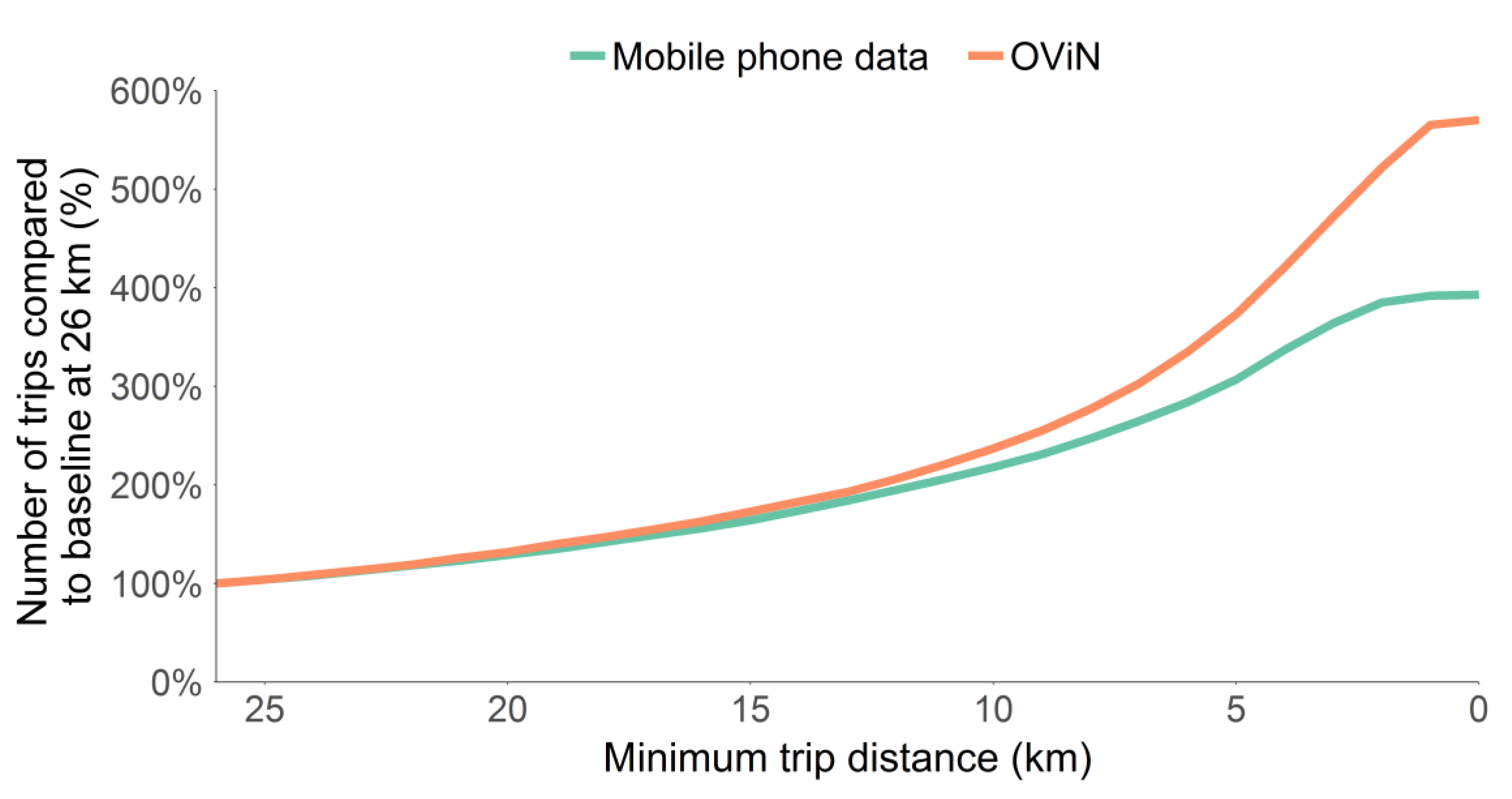
When compared to OViN we see a similar distribution of the number of trips on longer distance classes, but diverging trip counts for trips below 10 km, shown in Figure 4. The comparison with OViN is made by setting the total trips over 26 km as a baseline (100%) and comparing this to the total number of trips including shorter distances. 26 km is chosen as the largest destination in our mobile phone data is 26 km in diameter. Hence, a person is able to travel at most 26 km without being recorded traveling.

We find there are about as many trips in both datasets over 10 km, though below 10 km OViN appears to record far more trips. Hence, we choose to only take trips over 10 km into account as we have an underrepresentation below 10 km. This is also a bias that is hard to correct for provided it depends on the physical cell tower infrastructure. In areas with larger reaching cell towers one might never be able to detect short trips, whereas in cities with smaller cells one might. Hence, we only look at trips over 10 km and focus on measuring mobility on highways, where trips are typically greater than 10 km.

3.2. Scaling Mobile Phone Data

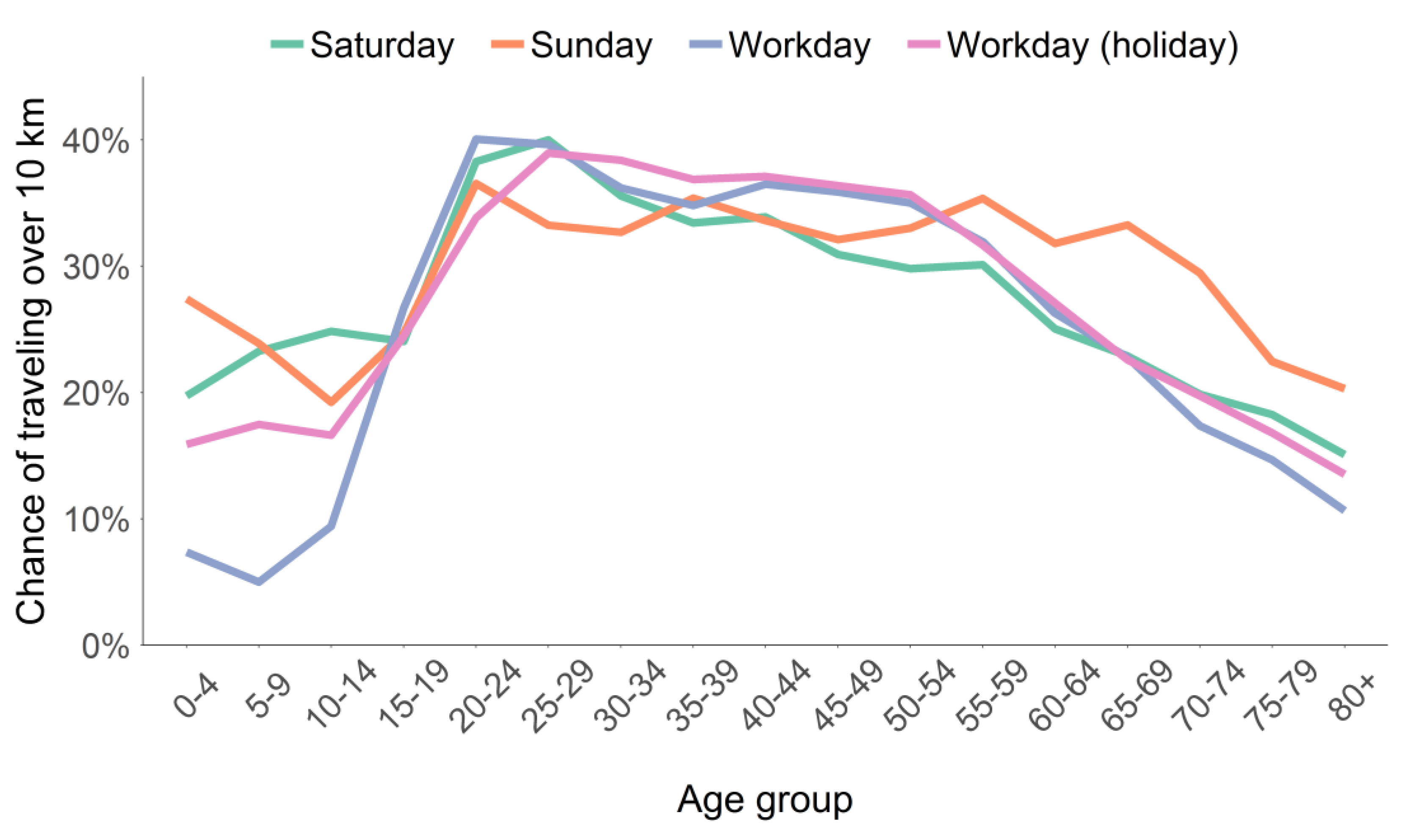
The scaling method comprises both a bias correction as well as expanding the counts to approach those in the true population. This method corrects for demographic differences in the population that affect the probability that a person is recorded in our sample when performing a trip. The probability of being observed traveling depends on two factors: (1) the chance of being in the sample and (2) the chance of traveling. Both these factors are dependent upon inhabitant demography and type of day. Children under the age of 10, for example are both less likely to own a mobile phone and to be found traveling on highways [17]. Consequently they are both less likely to be present in the sample and less likely to be found traveling over 10 km. Moreover, the chance children are traveling longer distances differs between schooldays, holidays and weekends. The likelihood of a person taking a trip of at least 10 km or more for a range of age groups is shown in Figure 5.

Note we focus on trips over 10 km as trips below 10 km are underrepresented in the mobile phone data. Hence, we choose not to use that information. From Figure 5 can be observed there are strong differences in travel behaviour between age groups. Our scaling method is designed to take these effects into account and adjust trip counts accordingly.

We make a distinction between four types of days. These are workdays, Saturdays, Sundays, and workdays during holidays. These day types provide insights into the distinct travel behaviours, with differences mainly observed for the young and old inhabitants. Further distinctions in day types did not provide additional information and would decrease the number of observations per group to the point where the group sizes are too small to extract stable and trustworthy values.

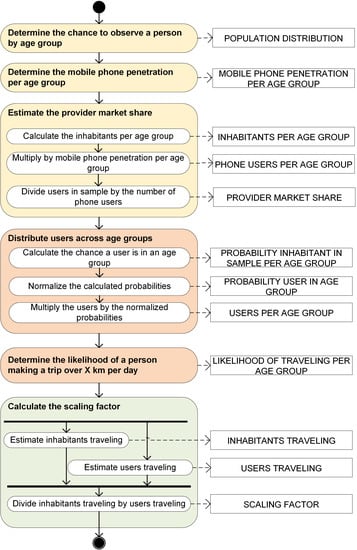
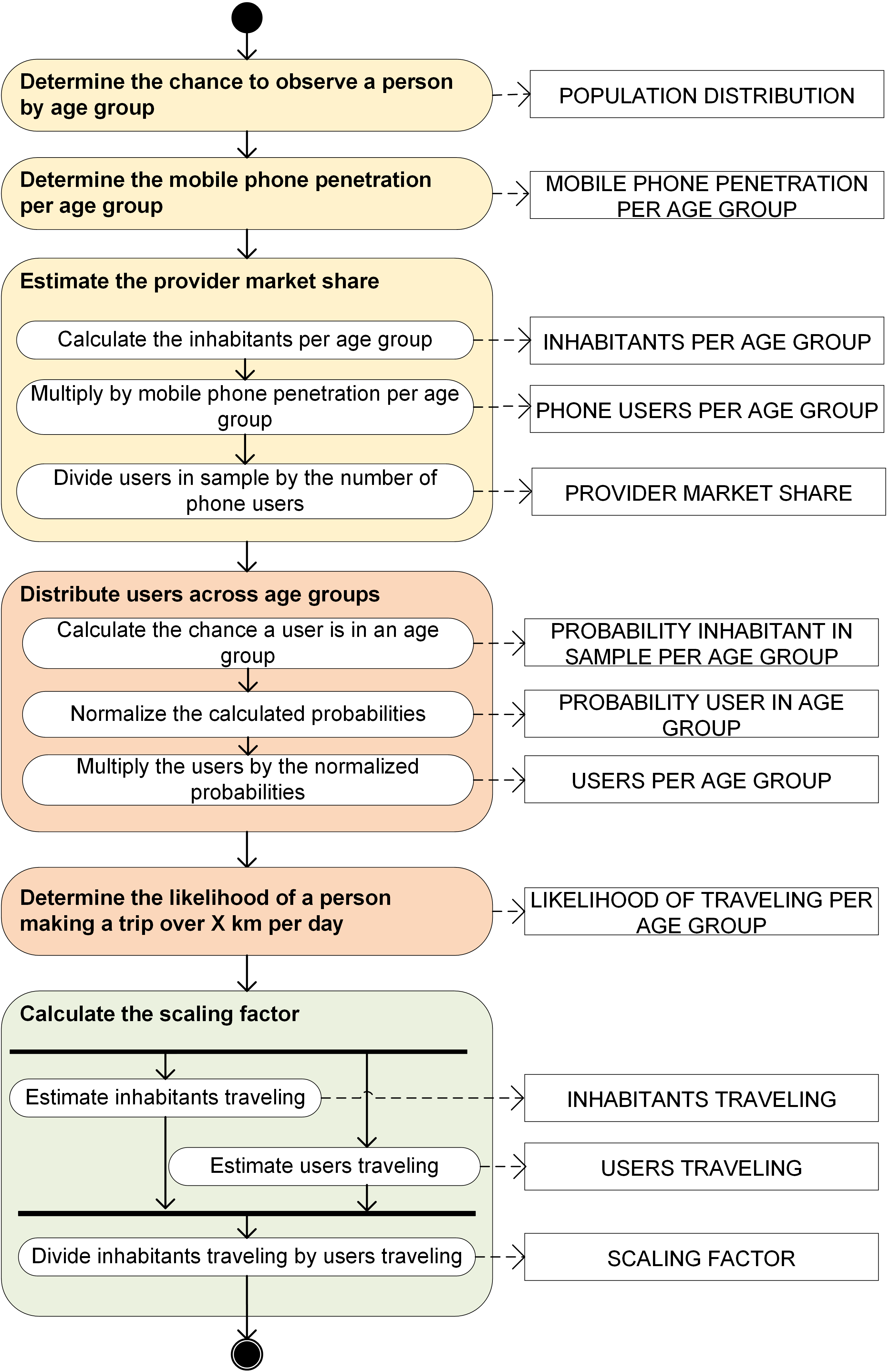
The proposed scaling method is formally represented in Figure 6 as a Meta-Algorithmic Model (MAM) in Process Deliverable Diagram (PDD) notation [33]. In a PDD the processes are shown on the left and the product of the action on the right [34]. The PDD is accompanied by two tables, one describing the processes (Appendix A,

Table A1. Activity table associated with the Meta-Algorithmic Model shown in Figure 6.

ACTIVITY	SUB-ACTIVITY	DESCRIPTION
DETERMINE THE CHANCE TO OBSERVE A PERSON BY AGE GROUP		Divide the number of people per age group by the total number of inhabitants in that area.
DETERMINE THE MOBILE PHONE PENETRATION PER AGE GROUP		Retrieve data concerning the mobile phone penetration per age group from (a) trusted source(s).
ESTIMATE THE PROVIDER MARKET SHARE	Calculate the inhabitants per age group	Multiply the total number of inhabitants by the POPULATION DISTRIBUTION. Note, the total number of inhabitants used here is adjusted for people being abroad, on a holiday, or on a business trip (Geerts, 2014).
	Multiply by mobile phone penetration per age group	Multiply the INHABITANTS PER AGE GROUP by the MOBILE PHONE PENETRATION PER AGE GROUP.
	Divide users in sample by the number of phone users	Divide the number of users in the area by the number of phone users in the area, i.e., the sum of the PHONE USERS PER AGE GROUP.
DISTRIBUTE USERS ACROSS AGE GROUPS	Calculate the chance a user is in an age group	Multiply the POPULATION DISTRIBUTION by the MOBILE PHONE PENETRATION PER AGE GROUP and by the PROVIDER MARKET SHARE.
	Normalize the calculated probabilities	Divide the PROBABILITY INHABITANT IN SAMPLE PER AGE GROUP by the sum of the PROBABILITY INHABITANT IN SAMPLE PER AGE GROUP.
	Multiply the users by the normalized probabilities	Multiply the users in the area by the chance of observing a user in a certain age group, i.e., the PROBABILITY USER IN AGE GROUP.
DETERMINE THE LIKELIHOOD OF A PERSON MAKING A TRIP OVER X KM DURING WORKDAYS, WORKDAYS DURING THE HOLIDAY, SATURDAYS, AND SUNDAYS PER AGE GROUP		Gather information about the chance that a person of a certain age groups makes a trip longer than X kilometres on a day. We use OViN to determine this and take the differences in weekday, weekend, and holiday separately into account.
CALCULATE THE SCALING METHOD	Estimate inhabitants traveling	Multiply the INHABITANTS PER AGE GROUP by the LIKELIHOOD OF TRAVELING PER AGE GROUP.
	Estimate the users traveling	Multiply the USERS PER AGE GROUP by the LIKELIHOOD OF TRAVELING PER AGE GROUP.
	Divide inhabitants traveling by users traveling	Divide the sum of the INHABITANTS TRAVELING by the sum of the USERS TRAVELING.

) and one describing the products (Appendix A,

Table A2. Concept table belonging to the PDD shown in Figure 6.

CONCEPT	DESCRIPTION
POPULATION DISTRIBUTION	The probability that an inhabitant belongs to a certain age group.
MOBILE PHONE PENETRATION PER AGE GROUP	The probability that a Dutch citizen of a certain age group possesses a mobile phone.
INHABITANTS PER AGE GROUP	The absolute number of inhabitants per age group.
PHONE USERS PER AGE GROUP	The absolute number of inhabitants that possess a mobile phone per age group.
PROVIDER MARKET SHARE	The market share of the network provider. Hence, in this case the market share is equal for all age groups.
PROBABILITY INHABITANT IN SAMPLE PER AGE GROUP	The probability that an inhabitant is in our sample per age group.
PROBABILITY USER IN AGE GROUP	The probability that a user in our sample is in a certain age group.
USERS PER AGE GROUP	The absolute number of users per age group.
LIKELIHOOD OF TRAVELING PER AGE GROUP	The probabilities that a person of a certain age group makes a trip that is longer than X kilometers on a specific day of the week.
INHABITANTS TRAVELING	The number of INHABITANTS PER AGE GROUP that is expected to make a trip over X kilometers on a specific day of the week.
USERS TRAVELING	The number of USERS PER AGE GROUP that is expected to make a trip over X kilometers on a specific day of the week.
SCALING METHOD	The ratio between the number of INHABITANTS TRAVELING the number of USERS TRAVELING. The scaling methods applies to traveling people, because these are the people that are relevant for the OD matrix.

). The next paragraphs will provide a brief overview of the steps and products in the scaling method.

As shown in the MAM with the different colour codes there are three types of steps in the scaling method. The first is represented with yellow concerns acquiring information about the population for all relevant areas. In addition we also estimated the number of mobile phone users living in each area by assigning a home location to each user. This is done using a slight variation of the home assignment algorithm described by Toole et al. [11]. Whereas Toole et al. assigned home as the most frequent stay location between 8 pm and 7 am on workdays we also include data about weekends, but the differences are minor [11]. A user is assigned one home location for the month October 2015. Home locations are key to determine the distribution of users across the country and hence the ratio mobile phones in the sample over the inhabitants for all areas.

The second step in our method shown in red is the difference between traveling and general population. Here we first estimated the age distribution within our sample by looking at the a-priori information about the population distribution in the area’s population and the chance of owning a smartphone per age group. This helped us to calculate the number of users per age group. For each of these age groups we can predict how likely they are to be found traveling for a specific day type.

The final step is what differentiates our scaling method from those in previous studies. Here we calculate how many inhabitants and mobile phone users in our sample are expected to travel over 10 km. In the end we divide the inhabitants we expect to be traveling by those we expect to be traveling within our sample. The calculated ratio will be the scaling factor for a specific area on a specific day.

3.3. Validating the Scaling Method using Roadside Measurements

There are four essential steps required to measure vehicles on highways using mobile phone data: (1) scale the mobile phone data to the population, (2) focus on the vehicle trips, (3) select the vehicle trips going over a specific road, and (4) convert trips into vehicles. The first step, i.e., scaling, was covered in the previous section and will not be discussed here. The latter three will be discussed in the following paragraphs.

The algorithm by Keij [31] is implemented to distinguish train trips from vehicle trips. Note that there might also be other categories, e.g., cycling, that are not included. This is a slight shortcoming, though given our focus on longer trips in combination with highways we expect the majority not to be cycling. The basis of the algorithm is detecting whether events occur with cells covering only highways or only rail tracks [31]. Especially on longer distances the algorithm is shown to provide good results [31].

We are interested solely in a subset of all car trips. These are the ones passing over specific road section where also roadside measurement data is available. Hence, we need to make an educated guess on the route people travel from their origin to destination. Once we got a good idea of the routes travelled we can select all origin destination combinations that cross a specific road section. This provides an estimate of all people who travel over the road network and plausibly cross a specific road. Next, we will assign a time stamp to these trips defined as the middle of their trip, e.g., trips leaving at 8:00 AM and arriving at 9:00 AM will cross the road section at 8:30 AM. This is not very precise, but as some trips will in reality cross the road section earlier and other later we are confident the majority of the uncertainty will level out.

A major step in the above process is acquiring routes for origin destination pairs. There is a large volume of published studies describing how to assigning vehicle trips from Origin Destination pairs (OD-pairs) [35,36]. A key assumption that is often made is that people are rational and take the route that minimizes their travel cost [35]. Travel cost can be seen as a combination of multiple factors such as travel time, distance, cost of fuel, congestion charges, et cetera [35]. The most important factors, explaining 60% to 80% of all route choices in practice, are travel time and distance [35]. Methods taking the shortest path or k shortest paths as the possible route choices between OD-pairs account for the largest group of path generation methods [36]. At the moment the dataset available for this study uses Dijkstra’s shortest time path algorithm to link OD-pairs to road sections [37]. The shortest time path is chosen by time rather than distance. This is done by taking into account the maximum speed allowed on a road section based on the information from Open Street Maps (OpenStreetMap contributors, 2014). We provided a 20% discount for travel times on highways provided people prefer to stay on highways when the time benefits are minimal [38]. The 20% will account for this.

The conversion factor is applied as calculated in Section 2.3. Note here we said the people per vehicle ratio depends on trip motives. Trip motives are inferred from the mobile phone data based on trip characteristics [39]. A detailed description of the algorithm used can be found in Van Langen [39]. After applying the algorithm to our dataset we could simply use our conversion factors to go from trips to vehicles.

3.4. Prepare Roadside Measurement Data

Raw data is provided by NDW [29] in xml format and converted to a manageable csv using software written in Python [40]. The csv contains information about the measurement site as a whole for 15 minute periods, e.g., the average vehicle count or average velocity. In addition, it contains information about the minimum and maximum vehicle counts and velocities as well as information on the number of trucks passing by. To keep data manageable, information about the independent lanes are aggregated to a single vehicle count.

3.5. Filtering Untrustworthy Roadside Measurement Data

To ensure data quality we constructed two criteria the roadside measurement sites have to meet before taking them in contention for the comparison with mobile phone data.

The first criterion is that a 15 minute interval may at most lack 6 minutes of erroneous data within the roadside measurement data. Standard deviations of on average 4.5% between differences in vehicle counts are found by comparing values from consecutive measurement sites, i.e., where no off-ramp or on-ramp separates the measurement points. The latter is done such that the same amount of vehicles are destined to travel by both measurement sites. As a result the difference in reported vehicle counts can only be explained by errors in measurement. The 4.5% is found by comparing consecutive measurement sites at 30 locations. When the error in measurement of each site is normally distributed and equal amongst sites, the standard deviation for each measurement site becomes approximately 3.2% following the variance sum law. This is very acceptable and provides us with a good indication of how accurate the roadside measurements are.

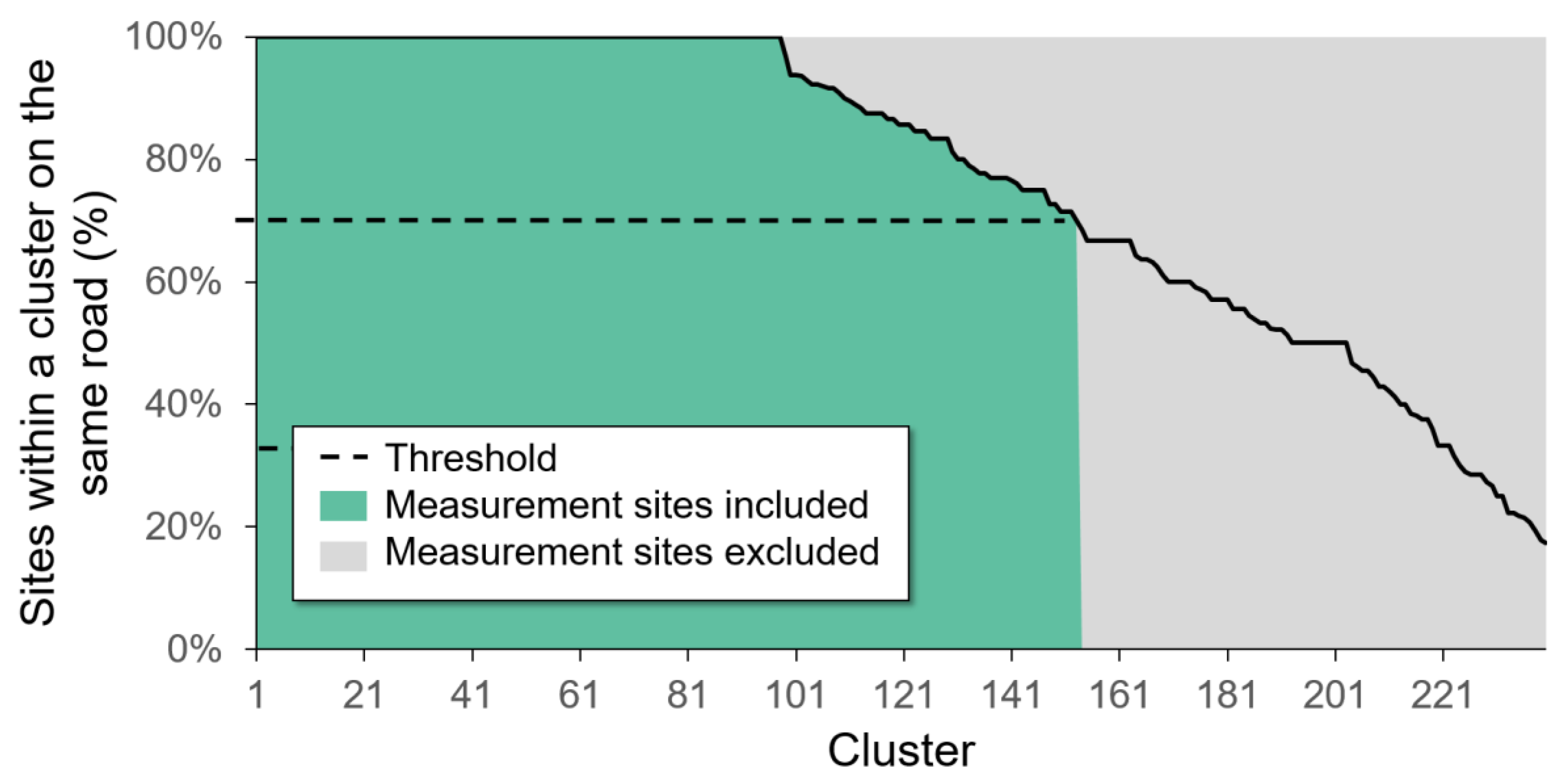
The second criteria is slightly more complicated and relates to our suspicion that the location of measurement sites are not always accurately represented in the database. To test whether sites are on the reported location we performed a test based on the following premise: measurement sites that are located on the same road near each other will produce more similar vehicle counts than measurement sites further apart. The idea is to (1) cluster measurement sites based on their vehicle counts, here we opted for k-means clustering, and (2) check if sites within each cluster are located on the same road, e.g., the A4, as reported by the NDW [41].

For clustering we used vehicle counts of 145 hours during October 2015 where all 4.775 sites are without missing data. The vehicle counts are then normalized per hour. For clustering we set the number of clusters equal to 240, leaving us with approximately 20 measurement sites per cluster. The results are shown in Figure 7. We observe the majority of the clusters have over 70% of the measurement sites on the same road and also headed in the same direction, e.g., North. The 70% we use as a threshold, when less than 70% of the sites on one cluster are located on different roads we are unsure about their locations. Only the sites belonging to clusters with the majority (70%) of the measurement sites on the same stretch of road meet our second criteria.

In the end both criteria leave us with 1.761 measurement sites. The majority are discarded for having more than 6 minutes of erroneous data within 15 minute intervals for 95% of the recorded hours. These measurement sites are less accurate in general and hence are not the gold standard we are looking for. The final 140 measurement sites are discarded due to the second criteria as we are not sufficiently confident that their reported location is correct.

3.6. Comparison of Vehicle Counts

The final comparison will compare vehicles measured from the scaled mobile phone data in contrast to the vehicles recorded by the NDW, i.e., the roadside measurement data.

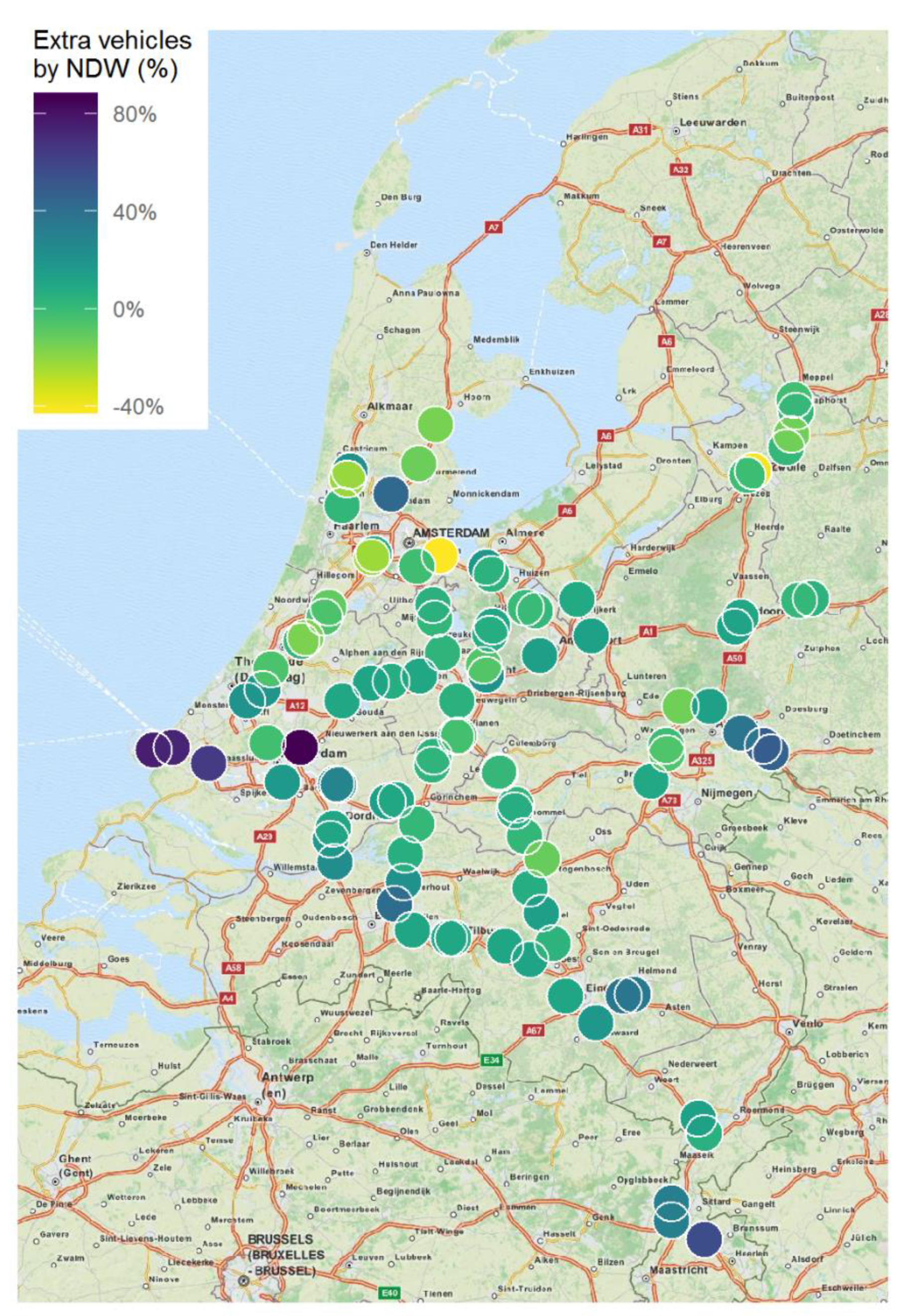
In total 100 comparison sites are nearly randomly selected. We put one constraint on the measurement sites to ensure we get a better sample of the Netherlands in general. As the government is most interested in traffic intensities on busier roads, there are many more data points near and between the larger cities in the Netherlands. If we would randomly select measurement sites, the majority would be near and in between these cities. Hence, we ensured there are no measurement sites on the same road, headed in the same direction, within 10 km from other measurement sites in the sample. Sites are randomly drawn from the 1.761 measurement and added to our sample if there is no overlap within 10 km with other sites in the sample. The resulting measurement sites are depicted in Figure 8.

Vehicle counts will be compared on measurement site, weekday, and hour level. The main metric using in the analysis is the ‘Extra vehicles on the road by NDW (%)’. This is a value is calculated as described in Equation (1), where E stands for ‘Extra vehicles on the road by NDW (%)’, NDW is the number of vehicles measured via roadside measurement devices, and M stands for vehicles inferred from the scaled mobile phone data.

$$E=\frac{\mathrm{NDW}-\mathrm{M}}{NDW}$$

(1)

4. Results

The first analysis we performed is on measurement site level. In Figure 8 the extra vehicles on the road by NDW (%) is represented for all 100 measurement sites. The majority of locations show the vehicle counts are nearly equal between the two data sources.

Unfortunately, there are differences in vehicle counts on several locations on the Dutch highways. The mobile phone data underestimates the number of vehicles on the road near the country’s borders. Where the country borders Belgium and Germany we see darker bluish colours indicating there are less vehicles measured via mobile phone data. This may be due to people switching off their phones while being or going abroad, resulting in an underrepresentation of the sample. Furthermore, on the left there are a few dark spots where land meets ocean. Here the routing algorithm in combination with the relatively low spatial resolution is the culprit. There are few routes crossing roads near the country borders and hence few trips will be assigned to these roads. With the current dataset the mobile phone data will not provide good estimates of traffic on roads near the border, which is a limitation we have to take into account. Nevertheless, it does work very well in the majority of the country.

Finally, we see two outliers in the form of one dark dot near Rotterdam and two yellow dots, one near Amsterdam and one near Zwolle. Provided they are surrounded by measurement sites that do show good results we can only imagine some bad roadside measurement sites slipped through our filters or the routing algorithm made some very local mistakes. In the further analyses the measurement sites where the the extra vehicles on the road by NDW (%) is over 20% or below -20% are removed either because they are outliers or because they show deviations not related to faults in the scaling method under investigation. This reduces our sample by 26 locations to a total of 74.

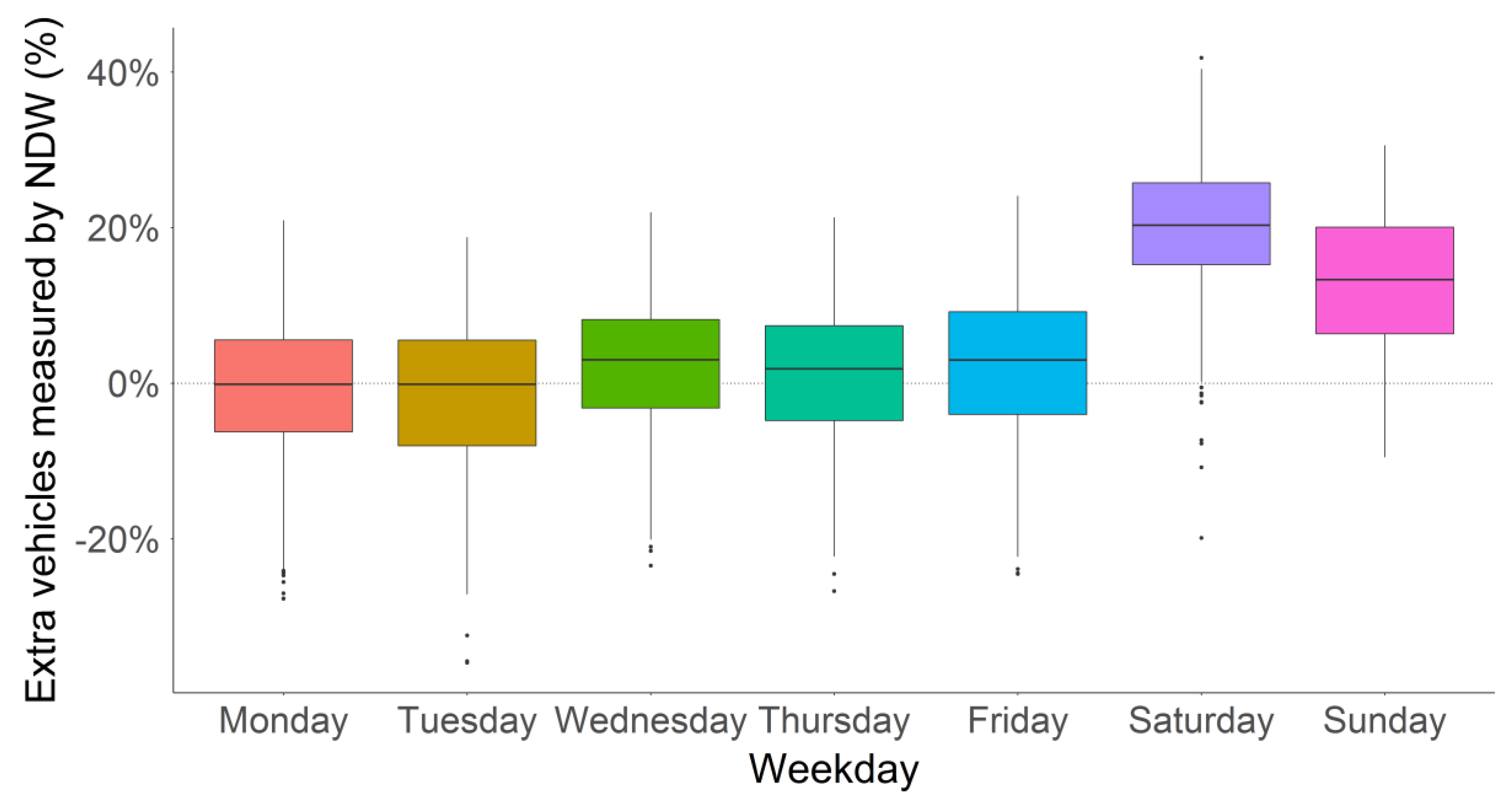
The second comparison made relates to differences between different weekdays. Each datapoint in Figure 9 represents the extra vehicles measured by NDW (%) per weekday per comparison location. The information is visualized in box whisker plots with outliers shown as dots outside the box whisker plots. Outliers here are defined as values deviating more than 1.5 times the Inter Quartile Range (IQR). For weekdays the scaled mobile phone data shows solid results. During Mondays and Tuesdays especially the number of vehicles inferred from the mobile phone data near perfectly matches the number of vehicles measured by roadside measurement devices. There is some variation, although this could also be the result of deviations from the shortest time path in the applied routing algorithm.

What is striking though, is the large deviations during weekend days. On Saturday especially the extra vehicles measured by NDW (%) is more often than not over 20%. For this we do not yet have a solid explanation, merely a few hypotheses. The most logical hypothesis, also in the trend of this paper, would be a bias in our sample. We expect there are people who use their mobile phone only for work purposes. These people might leave there phone at work or at home during the weekend. As we would expect some of these mobile phone would be traveling we overestimate the expected number of trips. As a result the scaling factor, i.e., the ratio expected traveling inhabitants over mobile phones traveling, is lower than it should be during the weekend. Alternatively, this may have to do with a mistake in our people per vehicle ratio, which is much higher during the weekend. There are less working people, and much more recreational traffic where OViN tells us there are more people per vehicle on average. The exact reason for the lower counts during weekends will have to be investigated in future research.

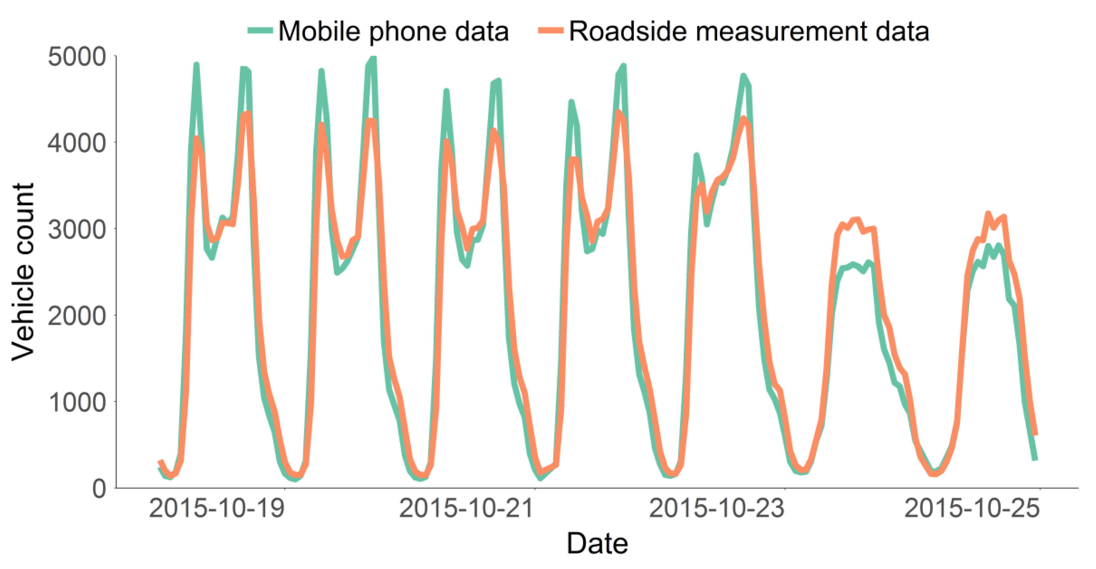
The final comparison we made is between hourly vehicle counts. This is done to get a grasp on how vehicle counts compare by hour. For this we selected a week in October 2015 and aggregated the counts per data source on hourly level. The results are shown in Figure 10.

On hourly level the vehicle counts between both data sources follow the same general pattern indicating that not only on weekday level, but also hour level, the scaling method correctly scales sample to the population. In fact on hour level the Pearson’s correlation coefficients are consistently above 0.87 and are 0.95 on average. Nevertheless, there are some discrepancies. The vehicle count during weekend days, as we know from the previous analysis, is slightly too low in the mobile phone data. This, however, appears to primarily affect the day time. Night time values for both work and weekend days are very evenly matched. Moreover, there appears to be a structural overestimation of vehicle counts during workday rush hours. Rush hour peaks during workdays are higher in the mobile phone movement data on every workday with the differences being approximately 20%. Note, however, during hours surrounding the peaks there are more vehicles measured via roadside measurements. Our best guess is that our time stamping technique, i.e., middle of the trip assignment, is to blame. When people get stuck in traffic and travel times increase our time stamping technique becomes less accurate. When people leave work at 5:00 PM and get home by 7:30 PM we guess they passed a road section by 6:15 PM while in fact this may be much earlier or later. For each specific point the delay may be skewed one way or the other. In our aggregation this would lead to more spread and lower peaks in traffic intensities as observed in Figure 10.

5. Conclusions

The results of this research are very promising. With the exception of road segments near the country border, the vehicles inferred from trips in the mobile phone data matches those from roadside measurements. This proves the scaling method we present and implement in this research allows us to measure mobility patterns and traffic intensities on highways using mobile phone data. Nevertheless, there is still some work to do with a slight underestimation of traffic intensities during the weekend and overestimation during workday peak rush hour traffic.

In this research we aimed to complement the vast amount of studies investigating and reporting the potential and possible applications for mobile phone data [3,14,16]. We did so by focussing and refining a crucial step in translating the sample to the traveling population. We identified a bias in that people more likely to travel are also more likely to own a phone, leading to potential overestimations of the traveling population. To correct for the bias we devised and presented a new scaling method that can be implemented in future studies. Using this scaling method showed mobile phone data can accurately measure traffic intensities without post calibration with, for example, roadside measurements. The latter implies the created scaling method is able to explain and account for the majority of biases in the data.

The results of this study provided answers, but also introduced new questions to investigate. During the daytime on weekend days, for one, the scaled mobile phone data appeared to underestimate the roadside measurements by 5% to 25%. Our best guess is that business users will have a separate phone for private use and will leave their work phone at home or at work during the weekend. This might explain why we underestimate trips during the weekend. Alternatively, the scaling method might be correct and the people per vehicle ratio extracted from OViN, which is much higher during the weekend, might cause this. How to correct for the bias in the weekend is to be answered by future research. Furthermore, mobile phone data has an underrepresentation of trips on shorter distances. Hence, we focused on highways and only included trips over 10 km. Although some research has been performed on this topic, we think it is worthwhile to further investigate this and add the required steps to correct for the bias in the scaling method proposed in this research.

The proposed and evaluated scaling method presented in this research can help us to get a better grasp of the traveling population. Demographic biases are accounted for leaving future researchers and policy makers with a less biased view of the population allowing them to make better judgements. When traffic models are created or calibrated with mobile phone data the scaling method could help to add provide more accurate information. Furthermore, the scaling method relies solely on information that is often widely available. When there is no other data source for calibration, e.g., in underdeveloped parts of the world, mobile phone data can still provide proper insights in the population’s mobility patterns.

References

- Fiedler, K. Beware of samples! A cognitive-ecological sampling approach to judgment biases. Psychol. Rev. 2000, 107, 659. [Google Scholar] [CrossRef] [PubMed]
- Tversky, A.; Kahneman, D. Judgment under uncertainty: Heuristics and biases. Science 1974, 185, 1124–1131. [Google Scholar] [CrossRef] [PubMed]
- Ahas, R.; Aasa, A.; Roose, A.; Mark, U.; Silm, S. Evaluating passive mobile positioning data for tourism surveys: An Estonian case study. Tour. Manag. 2008, 29, 469–486. [Google Scholar] [CrossRef]
- Becker, R.A.A.; Cáceres, R.; Hanson, K.; Loh, J.M.M.; Urbanek, S.; Varshavsky, A.; Volinsky, C. A tale of one city: Using cellular network data for urban planning. IEEE Pervasive Comput. 2011, 10, 18–26. [Google Scholar] [CrossRef]
- Eskes, P.; Spruit, M.; Brinkkemper, S.; Vorstman, J.; Kas, M. The Sociability Score: App-based social profiling from a healthcare perspective. Comput. Hum. Behav. 2016, 59, 39–48. [Google Scholar] [CrossRef]
- Friso, K.; Oakil, A.T. Advances by using Mobile Phone Data in mobility analysis in the Netherlands. In Proceedings of the 6th International Conference on Models and Technologies for Intelligent Transportation Systems (MT-ITS), Cracow, Poland, 5–7 June 2019; pp. 1–7. [Google Scholar]
- Snijkers, G. Getting data for (business) statistics: What’s new? What’s next? In Proceedings of the European Conference for New Techniques and Technologies for Statistics (NTTS), Brussels, Belgium, 18–20 February 2009; pp. 18–20. [Google Scholar]
- Wang, Z.; He, S.Y.; Leung, Y. Applying mobile phone data to travel behaviour research: A literature review. Travel Behav. Soc. 2018, 11, 141–155. [Google Scholar] [CrossRef]
- Astarita, V.; Florian, M. The use of mobile phones in traffic management and control. In Proceedings of the ITSC 2001, 2001 IEEE Intelligent Transportation Systems, Oakland, CA, USA, 25–29 August 2001; pp. 10–15. [Google Scholar]
- Cáceres, N.; Wideberg, J.P.P.; Benitez, F.G. Deriving origin destination data from a mobile phone network. Intell. Transp. Syst. IET 2007, 1, 15–26. [Google Scholar] [CrossRef] [Green Version]
- Toole, J.L.; Colak, S.; Sturt, B.; Alexander, L.P.; Evsukoff, A.; González, M.C. The path most traveled: Travel demand estimation using big data resources. Transp. Res. Part C Emerg. Technol. 2015, 58, 162–177. [Google Scholar] [CrossRef]
- Gonzalez, M.C.; Hidalgo, C.A.; Barabasi, A.L. Understanding individual human mobility patterns. Nature 2008, 453, 779–782. [Google Scholar] [CrossRef] [PubMed]
- Rathore, M.; Paul, A.; Ahmad, A.; Jeon, G. IoT-based big data: From smart city towards next generation super city planning. Int. J. Semant. Web Inf. Syst. 2017, 13, 28–47. [Google Scholar] [CrossRef] [Green Version]
- Jiang, S.; Ferreira, J., Jr.; González, M.C. Activity-Based Human Mobility Patterns Inferred from Mobile Phone Data: A Case Study of Singapore. In Proceedings of the International Workshop on Urban Computing, rbComp’15, Sydney, Australia, 10 August 2015. [Google Scholar]
- Cools, M.; Moons, E.; Wets, G. Assessing the impact of weather on traffic intensity. Weather Clim. Soc. 2010, 2, 60–68. [Google Scholar] [CrossRef] [Green Version]
- Iqbal, M.S.; Choudhury, C.F.; Wang, P.; González, M.C. Development of origin–destination matrices using mobile phone call data. Transp. Res. Part C Emerg. Technol. 2014, 40, 63–74. [Google Scholar] [CrossRef] [Green Version]
- Telecompaper. Smartphone Penetration Netherlands 2015 Q3 (Tech. Rep.); Telecompaper: Southwark, UK, 2015. [Google Scholar]
- Caceres, N.; Romero, L.M.; Benitez, F.G. Exploring strengths and weaknesses of mobility inference from mobile phone data vs. travel surveys. Transp. A Transp. Sci. 2020, 16, 574–601. [Google Scholar] [CrossRef]
- Martín, J.; Khatib, E.J.; Lázaro, P.; Barco, R. Traffic monitoring via mobile device location. Sensors 2019, 19, 4505. [Google Scholar] [CrossRef] [PubMed] [Green Version]
- Nihan, N.L.; Wang, Y.; Zhang, X. Evaluation of Dual-Loop Data Accuracy Using Video Ground Truth Data; No. WA-RD 535.1; Transportation Northwest, Department of Civil Engineering, University of Washington: Seattle, WA, USA, 2002. [Google Scholar]
- van Lint, J. Evaluatie en Analyse van Reisinformatie. MSc Thesis, Afdeling Transport & Planning, Faculteit Civiele Techniek en Geowetenschappen, Technische Universiteit Delft, Delft, The Netherlands, 2006. [Google Scholar]
- CBS. Ontwikkeling Bodemgebruik in Nederland 1996–2000. 22 December 2003. Available online: https://www.cbs.nl/nl-nl/achtergrond/2003/52/ontwikkeling-bodemgebruik-in-nederland-1996-2000 (accessed on 14 May 2016).
- Statista. Mobile Phone Users in the Netherlands 2011–2019|Forecast. 2016. Available online: http://0-www-statista-com.brum.beds.ac.uk/statistics/274751/forecast-of-mobile-phone-users-in-the-netherlands/ (accessed on 10 May 2016).
- Statista. Smartphone Penetration 2012–2015|Netherlands. 2016. Available online: http://0-www-statista-com.brum.beds.ac.uk/statistics/488353/smartphone-penetration-netherlands/ (accessed on 10 May 2016).
- CBS Isreal. Censuses around the World. 2016. Available online: http://www.cbs.gov.il/census/census/pnimi_page_e.html?id_topic=5 (accessed on 11 May 2016).
- Centraal Bureau Statistiek (CBS). Onderzoek Verplaatsingen in Nederland 2010. 2011. Available online: https://www.cbs.nl/-/media/imported/onze-diensten/methoden/dataverzameling/aanvullende-onderzoeksbeschrijvingen/documents/2011/37/2010-ovin-onderzoeksbeschrijving-art.pdf (accessed on 26 April 2020).
- Otten, M.B.J.; ‘t Hoen, M.J.J.; Den Boer, L.C. STREAM Personenvervoer 2014 VERSIE 1.1. 2014. Available online: https://www.ce.nl/publicaties/1478/stream-personenvervoer-2014-versie-11 (accessed on 26 April 2020).
- Offermans, M.; Priem, A.; Tennekes, M. Rapportage Project Impact ict; Mobiele Telefonie; Programma Impact ICT, Research report nr. 9; CBS: The Hague, The Netherlands; Heerlen, The Netherlands, 2013.
- Nationaal Databank Wegverkeersgegevens (NDW). MST—Dit Bestand Geeft Aan Waar de NDW Meetlocaties zich Bevinden. Nationaal Databank Wegverkeersgegevens. 2015. Available online: http://www.ndw.nu/documenten/ (accessed on 26 April 2020).
- Nationaal Databank Wegverkeersgegevens (NDW). Datalevering. 2015. Available online: http://www.ndw.nu/pagina/nl/103/datalevering/ (accessed on 26 April 2020).
- Keij, J. Smart Phone Counting: Location-Based Applications Using Mobile Phone Location Data. Master’s Thesis, Delft University of Technology, Delft, The Netherlands, 2014. Unpublished. [Google Scholar]
- Van Kats, J. Supporting Incident Management with Population Information Derived from Telecom Data. Master’s Thesis, Utrecht University, Utrecht, The Netherlands, 2014. Unpublished. [Google Scholar]
- Spruit, M.; Jagesar, R. Power to the People! Meta-algorithmic modelling in applied data science. In Proceedings of the 8th International Joint Conference on Knowledge Discovery, Knowledge Engineering and Knowledge Management KDIR 2016, 11–13 November 2016; ScitePress: Porto, Portugal, 2016; pp. 400–406. [Google Scholar]
- Van de Weerd, I.; Brinkkemper, S. Meta-modeling for situational analysis and design methods. Handbook of Research on Modern Systems Analysis and Design Technologies and Applications; Information Science Reference (IGI): Hershey, PA, USA, 2008; pp. 35–54. [Google Scholar]
- Ortúzar, J.D.D.; Willumsen, L.G. Modelling Transport; Wiley: Hoboken, NJ, USA, 2011. [Google Scholar] [CrossRef]
- Prato, C.G. Route choice modeling: Past, present and future research directions. J. Choice Model. 2009, 2, 65–100. [Google Scholar] [CrossRef] [Green Version]
- Dijkstra, E.W. A note on two problems in connexion with graphs. Numer. Math. 1959, 1, 269–271. [Google Scholar] [CrossRef] [Green Version]
- Ziebart, B.D.; Maas, A.L.; Dey, A.K.; Bagnell, J.A. Navigate like a cabbie: Probabilistic reasoning from observed context-aware behavior. In Proceedings of the 10th International Conference on Ubiquitous Computing, Seoul, Korea, 21–24 September 2008; pp. 322–331. [Google Scholar]
- Van Langen, J.J. The Attractiveness of Cities. Master’s Thesis, Utrecht University, Utrecht, The Netherlands, 2016. Unpublished. [Google Scholar]
- Van Rossum, G.; Drake, F.L., Jr. Python Reference Manual; Centrum voor Wiskunde en Informatica: Amsterdam, The Netherland, 1995. [Google Scholar]
- Hartigan, J.A.; Wong, M.A. A K-means clustering algorithm. Appl. Stat. 1979, 28, 100–108. [Google Scholar] [CrossRef]
Figure 1.
People per vehicle ratio plotted for different trip motives averaged per hour of the day (source: OViN).
Figure 2.
Chance of owning a smartphone by age group (sources: Telecompaper, CBS).
Figure 3.
Overview of our research approach to compare vehicle counts from scaled mobile phone data and roadside measurement data (sources: CDR, NDW).
Figure 4.
Comparison between OViN and our CDR dataset of the relative number of trips per travel distance. Both datasets have their number of trips set to 100% at a travel distance of 26 km.
Figure 5.
Chance of observing a person making a trip over 10 km during a day depending on the age group and type of day (sources: CDR, NDW).
Figure 6.
Meta-algorithmic model (MAM) showing the scaling method that will provide a scaling factor used to expand the sample to the population.
Figure 7.
Percentage of sites at the same road and on in the same direction for all 240 clusters.
Figure 8.
Extra vehicles measured by NDW (%) for all 100 selected comparison locations.
Figure 9.
Differences in extra vehicles measured by NDW (%) per weekday.
Figure 10.
Aggregated vehicle counts for one week in October 2015 for both data sources.