Impact Evaluation of Bike-Sharing on Bicycling Accessibility

Abstract

The presence of bike-sharing has a significant influence on the ease of trips by bike, which is one critical aspect of bicycling accessibility (BAcc). The existing measurements of BAcc rarely consider the factor of ownership of bikes, which means that no distinction is made between private-bikes and shared bikes. To measure BAcc more fully, this paper proposes a method to evaluate the influences of bike-sharing on BAcc and to perform the method on a real-world case study in Beijing. It is found that bike-sharing has a boosting effect on BAcc, and the increased rate of BAcc is significantly affected by bicycling frequency and shared-bike availability. A case study in Beijing utilizing geo-location data collected from two major bike-sharing companies (OFO and Mo-bike) illustrates the significance of the impact of bike-sharing on BAcc and the necessity to include bike-sharing in the measurement of BAcc. Besides, the case study shows BAcc around the transit station is better than that over the whole area. Given that bicycling feeds transit, this research lays the foundation for analyzing the combination of bike-sharing and transit from the perspective of accessibility and can further support transportation planning.

1. Introduction

As a travel mode, bicycling has significant advantages for short trips, including having zero emissions, being quicker than walking, and improving health. It also provides an alternative to and a useful feeder mode for public transport [1]. The importance of bicycling mobility in urban areas has been particularly highlighted by the COVID-19 outbreak, during which many countries have experienced a surge in cycling, including China, Germany, Ireland, the United Kingdom, and the United States [2]. European member countries of the United Nations consider bicycles as a way towards a “green recovery” to make post-COVID-19 mobility more environmentally friendly, healthy, and sustainable [3].

Bicycling accessibility (BAcc), an essential indicator for measuring bicycling mobility, is defined as the convenience or ease of bicycling travel and usually considers travel time and travel cost. BAcc is often used in bicycle infrastructure, land use, and transportation system planning [4,5,6,7]. BAcc also provides a measure of feeder mobility because bicycling is a solution for transit’s “last mile” problem [8,9,10].

Bicycling mobility consists of two modes: private-bike and shared-bike. Bike-sharing systems, especially free-floating bike-sharing (FFBS) systems, have caused a surge in bike-sharing usage [11], indicating that FFBS has dramatically improved the convenience of bicycling and has become an integral part of bicycling mobility. Since the start of the COVID-19 pandemic, Meituan (former name: Mo-bike) has experienced a 187% increase in bike-sharing ridership in Beijing [12]. Private bikes and shared bikes jointly contribute to bicycling mobility. In areas that have launched or are about to launch bike-sharing systems, consideration of bike-sharing is vital to the accurate evaluation of BAcc and transit accessibility.

The concept of accessibility was first defined by Hansen [13], and all measures of accessibility are ad hoc and vary in different contexts [14]. Generally, accessibility measures the ease of reaching goods, services, activities, and destinations [15,16], considering transportation resources, travel time, travel distance, and travel cost [17,18]. More specifically, accessibility involves three factors: the spatial distribution of destinations, the ease of travelling to these destinations, and the activities at the destinations [19,20]. In this paper, BAcc represents the ease of reaching destinations by bike. It differs from the term “accessibility to bicycling,” which denotes the ease of reaching bicycling facilities [21], and the term “accessibility to activities by bike,” which denotes the potential number of activities that can be accessed by bike [5,22].

Studies of bike-related accessibility have two branches. The first is rooted in studying the distribution of activities to examine how many activities can be accessed and focuses on the evaluation of activity distribution and identification of opportunities to support urban land use planning [5,22,23]. The other branch focuses on the ease (travel time, travel distance, and travel cost) of travelling to destinations by bicycle. There are two influences upon the ease of bicycling: the bicycling network and the bike itself. In this branch, most studies focus on supporting road network planning decision-making by evaluating bicycling networks and facilities and investigating the impact of new bicycling networks on BAcc [6,7,24]. The travel characteristics of the various types of bike (private pedal bike, shared pedal bike, private electric bike, shared electric bike) differ in terms of travel time and travel cost. For example, electric bikes travel at higher speeds, resulting in reduced travel times and, therefore, increasing BAcc [25,26]. Similarly, shared bikes do not have purchase or maintenance costs [27], leading to differences in travel costs compared to private shared bikes.

BAcc is currently determined on the use of private bikes and rarely considers shared bikes. The private-bicycling group has a relatively fixed size and high frequencies of bicycling because travelers with lower bicycling frequencies have higher bicycling costs (the cost of using an available bike for a trip), causing most of them to choose other travel modes [27]. The high and concentrated frequency of private bicycling makes bicycling costs relatively low and very consistent. Therefore, when considering only private bikes, the inclusion of the cost of using an available bike in the calculation of BAcc is unnecessary, and traditional BAcc is only for travelers who use private bikes to travel. However, when a bike-sharing system is present, it provides a fixed cost of using an available shared bike which is independent of bicycling frequency and makes bicycling a competitive travel mode for travelers with a low bicycling frequency (e.g., tourists). Thus, the distribution range of travelers’ bicycling frequency expands. Some travelers use shared bikes, and some ride private bikes. Bicycling cost is no longer consistent among travelers. Therefore, bicycling cost should not be neglected when evaluating the BAcc of areas that have launched or are about to launch a bike-sharing system. This paper investigates the inclusion of the influence of bike-sharing in the determination of BAcc to make it more comprehensive. It provides the following contributions:

• This study proposes a more comprehensive method for measuring BAcc considering both private bike and shared bike. There are two points of difference from traditional BAcc: i) this method incorporates the impact of bike-sharing on BAcc, which was traditionally measured based only on private bikes; ii) the BAcc in this paper is for all travelers, no matter what kind of travel mode they use (cycling, walking, or other), while the traditional BAcc is only for travelers with private bikes.
• A real-world case study of BAcc in Beijing was conducted using geolocation data collected from two major bike-sharing companies (OFO and Mo-bike).
• The increase in BAcc due to bike-sharing and the factors influencing this increase were investigated.

The rest of this paper is organized as follows. Section 2 introduces a method to measure BAcc at the origin-destination (O-D) and locational levels and analyses the impact of bike-sharing on BAcc. Section 3 presents the case study of BAcc in Beijing, including data sources, sample selection, parameter specifications, and numerical analysis. The paper concludes with a summary of the study and identifies directions for future research.

2. BAcc Taking Bike-Sharing into Consideration

This section proposes a method for measuring BAcc by considering both shared and private bikes in the calculation. People can choose between the two modes, and therefore have two options for their trip. The development of indicators and methods for accessibility when multiple modes are available is challenging [28]. Different from “accessibility to activities by bicycling” and “accessibility to bicycle facilities,” bicycling accessibility measures the ease of reaching destinations by bike. The ease of traveling can also be measured by impedance, and some studies directly equate the ease of traveling with impedance [29]. This paper defines BAcc as an indicator of the ease of bicycling to destinations by mapping the impedance (i.e., the ease of bicycling to destinations) to [0, 1].

2.1. BAcc at the Origin-Destination (O-D) Level

This section presents the BAcc at the O-D level: $BAc{c}_{od}$. The $BAc{c}_{od}$ is defined as an indicator of the ease of bicycling from the origin (o) to the destination (d), based on travel time and travel cost.

2.1.1. Measurement of BAcc at the O-D Level

$BAc{c}_{od}$ decreases with increasing travel impedance between a specified O-D pair. There are many forms to express decay, such as power, exponential, and combined functions. The exponential decay form suggested by Hansen [13] is widely used. Fotheringham and O’Kelly [30] argued that, for short travel distances, the negative exponential function is more suitable than other options. The negative exponential form guarantees that the function value is in the interval [0, 1]. Therefore, this study used the negative exponential form in the expression of $BAc{c}_{od}$.

$$BAc{c}_{od}=exp\left(-\beta ·I{M}_{od}\right),\mathrm{and}I{M}_{od}=\alpha ·t_{od}+C_{od}$$

(1)

$I{M}_{od}$ is the impedance of cycling from O to D, the generalized travel cost which consists of the cost of travel time $t_{od}$ and the cost of bicycling $C_{od}$, which can be considered as the cost of using an available bike for a trip. $\alpha$ is a parameter to unify these two items and can be considered the time value of bicycling, a socioeconomic parameter the value of which varies for different groups of people. $\beta$ is a parameter to map $I{M}_{od}$ to [0, 1] as uniformly and reasonably as possible.

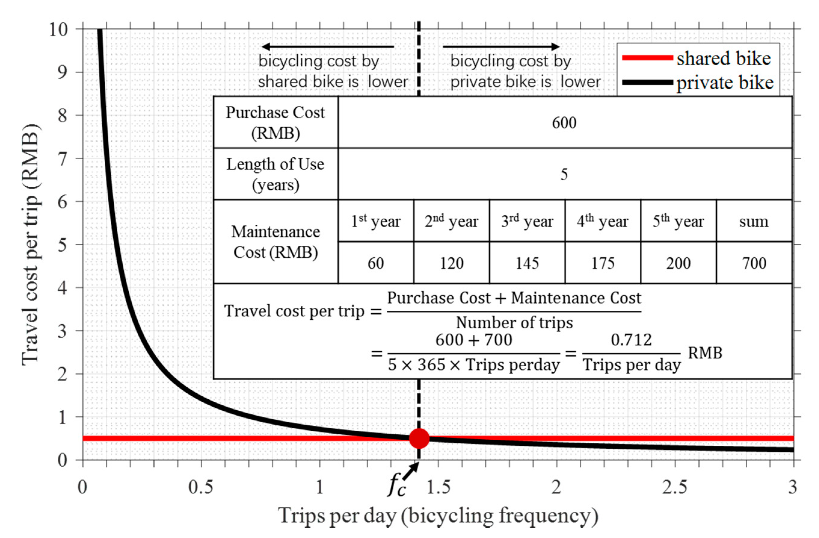
There is no difference in speed between private bikes and shared bikes, so the value of $t_{od}$ is the same for the two modes. However, they differ in $C_{od}$: the bicycling cost by shared bike is the booking fare; while the bicycling cost by private bike for a trip comes from the purchase and maintenance costs of a private bike and equals the value of amortizing the purchase cost to each trip (Figure 1). This difference in $C_{od}$ leads to a choice about which kind of bike (shared or private) should be selected for calculating $C_{od}$. Based on the principle of “interaction potential” [14], the mode with greater accessibility is used herein for the calculation of $BAc{c}_{od}$, i.e., the lower cost of bicycling with the two modes is the value of $C_{od}$.

The travel cost for a single trip was calculated instead of its travel distance, because bikes are usually used for trips of less than 5 km [31,32,33], and the range of travel distances is small. Based on the research by Song et al. [27], the bicycling cost of one trip by private bike was determined by vehicle purchase cost, maintenance cost, service life, and usage frequency. The calculation method of Song et al. [27] was utilised herein; bicycling cost with a private bike, $c_{private}=C_{private}^{day}/f$, where $c_{private}^{day}$, is the cost for owing a private bike for one day, and f is the bicycling frequency (number of trips by bike per day) with the density function $h\left(f\right)$. The bicycling cost of one trip by shared bike is the fare $c_{shared}$. Then $C_{od}$ can be expressed as

$$C_{od}=E\left[\left\{\underset{j\in s}{\min }{c}_j|s\in S\right\}\right]$$

(2)

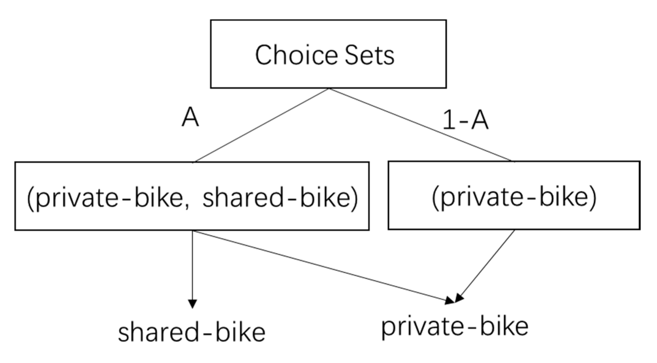
where $s$ denotes a choice set, $S$ is the set of choice sets, and $j$ indicates an alternative (travel mode) of $s$. It is worth noting that there is more than one choice set s because, if there is an available shared bike, the choice set is {private-bike, shared-bike}; otherwise, the choice set is {private-bike}.

In this study it is assumed that the private bike is always available, while the availability of a shared bike depends on the distribution of shared bikes. This is because the private bike’s availability depends on the traveller’s decision and they can purchase bikes and park them at trip origins to provide bike availability, i.e., the travellers determine the availability of private bikes and there are no restrictions for anyone to use an available private bike as long as he/she pays enough. However, travellers play a passive role in the availability of shared bikes, which are provided by external sources, such as operators of bike-sharing systems, and the traveller cannot use an available shared bike if there is no shared bike near the origin no matter how much he/she is willing to pay. Therefore, this study considers this from a long-term perspective. Perhaps a traveller has no purchased bike at his/her first trip. However, if owning a private bike is more suitable for him/her, he/she will buy one from a long-term perspective. The corresponding bicycling frequency is also long-term.

The elements in the two choice sets are determined by shared-bike availability (see Figure 2). $A_o$ (shared-bike availability) represents the probability that there is a shared bike available at the origin. The choice set (private bike, shared bike) represents a binary choice. Based on the study by Song et al. [27], $c_{private}$ will be less than $c_{shared}$ if the bicycling frequency is high enough (see Figure 1). When the choice set is (private bike), only private bikes are available.

For the group of travellers with bicycling frequencies distributed as $h\left(f\right)$, Equation (2) for determining $C_{od}$ can be rewritten as

$$\begin{array}{c}{C}_{od}=A_o·c_{shared}·{{\displaystyle \mathsf{\int }}}_0^{f_c}h\left(f\right)d_f+A_o·{{\displaystyle \mathsf{\int }}}_{f_c}^{+\infty }\frac{C_{private}^{day}}{f}·h\left(f\right)d_f\\ +\left(1-A_o\right)·{{\displaystyle \mathsf{\int }}}_0^{+\infty }\frac{C_{private}^{day}}{f}·h\left(f\right)d_f,\end{array}$$

(3)

where $f_c$ is the critical frequency at which the travel costs by private bike and shared bike are the same: $f_c=C_{private}^{day}/c_{shared}$. Further, $c_{shared}<c_{private}iff<f_c,$ and $c_{shared}>c_{private}iff>f_c$ (Figure 1 is an example).

2.1.2. The Impact of Bike-Sharing at the O-D Level

Bike-sharing affects $BAc{c}_{od}$ by changing bicycling costs. For travellers with a low bicycling frequency, shared bikes can dramatically reduce their bicycling cost, thus improving bicycling accessibility and attractiveness.

To measure the change in bicycling accessibility ($\mathsf{\Delta }BAc{c}_{od}$), the baseline scenario was set as no shared bikes, $A_o=0$. Equation (4) shows that $\mathsf{\Delta }BAc{c}_{od}$ is positive if $\mathsf{\Delta }{C}_{od}$ is negative. Equation (5) gives the rate of the increase in $BAc{c}_{od}$, which is determined by the value of $\left|\mathsf{\Delta }{C}_{od}\right|$; the larger $\left|\mathsf{\Delta }{C}_{od}\right|$ is, the higher the rate of increase. Equation (6) shows that $\mathsf{\Delta }{C}_{od}$ is non-positive, indicating that the presence of bike-sharing will reduce bicycling cost and, therefore, increase bicycling accessibility.

$$\mathsf{\Delta }BAc{c}_{od}=e^{\beta ·\left(\alpha ·t+C_{od}^{baseline}\right)}·\left(e^{-\beta ·\mathsf{\Delta }{C}_{od}}-1\right)$$

(4)

$$\frac{\mathsf{\Delta }BAc{c}_{od}}{BAc{c}_{od}^{baseline}}=e^{-\beta ·\mathsf{\Delta }{C}_{od}}-1$$

(5)

$$\mathsf{\Delta }{C}_{od}=A_o·{{\displaystyle \mathsf{\int }}}_0^{f_c}\left(c_{shared}-\frac{C_{private}^{day}}{f}\right)·h\left(f\right)d_f$$

(6)

$$\left|\frac{\mathsf{\Delta }{C}_{od}}{C_{od}^{baseline}}\right|=\frac{A_o·{{\displaystyle \mathsf{\int }}}_0^{f_c}\left(\frac{C_{private}^{day}}{f}-c_{shared}\right)·h\left(f\right)d_f}{{{\displaystyle \mathsf{\int }}}_0^{+\infty }\frac{C_{private}^{day}}{f}·h\left(f\right)d_f}$$

(7)

The term $\left|\mathsf{\Delta }{C}_{od}/C_{od}^{baseline}\right|$ in Equation (7) measures the magnitude of the travel-cost reduction. Equations (6) and (7) show that $\mathsf{\Delta }{C}_{od}$ and $\left|\mathsf{\Delta }{C}_{od}/C_{od}^{baseline}\right|$ are both affected by the supply of shared bikes ($A_o and c_{shared}$), the supply of private bikes (represented by $C_{private}^{day}$, including the purchase cost, repair cost and service life of the bike), and the bicycling frequency density function ($h\left(f\right)$). Shared-bike availability is the critical factor: when A = 0, there is no reduction in bicycling costs; the higher value of A, the more significant the travel-cost reduction. The upper limit of the travel-cost reduction is determined by $c_{shared}$, $C_{private}^{day}$, and $h\left(f\right)$. People with a high probability of $f<f_c$ have a significant reduction in travel cost, and as the expected value of $f$ approaches 0, the value of $\left|\mathsf{\Delta }{C}_{od}/C_{od}^{baseline}\right|$ approaches 100%. Higher values of $c_{shared}$ and $C_{private}^{day}$ correspond to higher travel costs. Based on the signs of their partial derivatives, $c_{shared}$ and $C_{private}^{day}$ have opposite effects on $\left|\mathsf{\Delta }{C}_{od}/C_{od}^{baseline}\right|$. An increase in $c_{shared}$ decreases $\left|\mathsf{\Delta }{C}_{od}/C_{od}^{baseline}\right|$; an increase in $C_{private}^{day}$ increases $\left|\mathsf{\Delta }{C}_{od}/C_{od}^{baseline}\right|$.

2.2. BAcc at the Locational Level

This section presents the measurement of BAcc at the locational level, representing the cumulative effects of bicycling accessibility. At the locational level, $BAc{c}_o$ is viewed as the ease of travelling by bike from an origin (o) to potential destinations based on travel time and travel cost.

2.2.1. Measurement of BAcc at the Locational Level

The value of $BAc{c}_o$ is the weighted accumulation of $\left\{BAc{c}_{od}|d\in D\right\}$, where D is the set of destinations corresponding to the o. The weight is set to be the probability of starting from o to d, and $BAc{c}_o$ is calculated as

$$BAc{c}_o={\displaystyle \sum }_{d\in D}BAc{c}_{od}·W_{od},$$

(8)

where $W_{od}$ is the weight for choosing d from D, corresponding to the travel demand, and is consistent with the trip distribution. Based on transportation planning theory, $W_{od}$ is determined by the attractiveness of the destination and the impedances from the origin to the destination. Gravity models are a popular method for trip distribution estimation; the one proposed by A.M. Voorhees is

$$N{T}_{od}=G_o\frac{A{T}_d·f(·)}{{{\displaystyle \sum }}_{d\in D}A{T}_d· f(·)},$$

(9)

where $N{T}_{od}$ is the number of trips from o to d, $G_o$ is the volume of trips generated at o, and AT_d is the attractiveness of d. $f(·)$ is the distributed impedance function. Generally, $f(·)$ considers factors such as travel distance, travel time, travel cost, and the number of transfers [34,35].

In this study, $G_o$ was set to be 1 to convert the $N{T}_{od}$ to a weight. $f(·)$ was set as a function of travel distance, and $f\left(L_{od}\right)=e^{-b · L_{od}}$, where b is a scaling parameter of travel distance, and $L_{od}$ is the travel distance between o and d. The weight $W_{od}$ can then be expressed as

$$W_{od}=\frac{A{T}_d· e^{-b · L_{od}}}{{{\displaystyle \sum }}_{d\in D}A{T}_d· e^{-b · L_{od}}}.$$

(10)

The parameter b must be estimated, for which the likelihood maximization method can be used, given an available data set of corresponding trip records. The likelihood function is $L={{\displaystyle \prod }}_i^I{W}_{i, od}$, where I is the set of travellers and $W_{i, od}$ denotes the probability of the person $i$ choosing d as their destination from o.

2.2.2. The Impact of Bike-Sharing at the Locational Level

At the locational level, the impact of bike-sharing on $BAc{c}_o$ combines the impacts on the multiple $BAc{c}_{od}$. values for possible destinations. The rate of increase is given by

$$\frac{\mathsf{\Delta }BAc{c}_o}{BAc{c}_o^{baseline}}=\frac{{{\displaystyle \sum }}_{d\in D}\left[\left(e^{-\beta ·\mathsf{\Delta }{C}_{od}}-1\right)·BAc{c}_{od}^{baseline}·W_{od}\right]}{{{\displaystyle \sum }}_{d\in D}BAc{c}_{od}^{baseline}·W_{od}}.$$

(11)

For the location o, the reduction in travel cost is fixed and does not change for different destinations. Equation (11) can then be expressed as

$$\frac{\mathsf{\Delta }BAc{c}_o}{BAc{c}_o^{baseline}}=e^{-\beta · \mathsf{\Delta }{C}_{od}}-1$$

(12)

The value of $\frac{\mathsf{\Delta }BAc{c}_o}{BAc{c}_o^{baseline}}$ equals the value of $\frac{\mathsf{\Delta }BAc{c}_{od}}{BAc{c}_{od}^{baseline}}$.

3. Case Study of BAcc in Beijing, China

This section presents a case study of BAcc in Beijing that illustrates the significant impact of bike-sharing on BAcc and the necessity of including bike-sharing in BAcc determinations. The bike-sharing systems in Beijing are free-floating, and the shared bike can be parked along the side of the road and in other public areas, not specified to a station or a specific place.

3.1. Data Sources

The data used in the case study were the parking locations of the shared bikes of Mo-bike and OFO, the two major bike-sharing operators in Beijing in 2015, in the area within Beijing’s fifth ring road. Shared-bike-location data is available for the public to examine in real-time. This study observed and collected 68 GB of data for one week in August 2015. This data included the parking locations of more than 850,000 shared bikes in the subject area, which were updated every seven min. The location data collected included the shared bike ID, the owner (operator), the time, and the longitude and latitude of the parking location. This data set was used to calculate shared-bike availability and to estimate the parameter $W_{od}$.

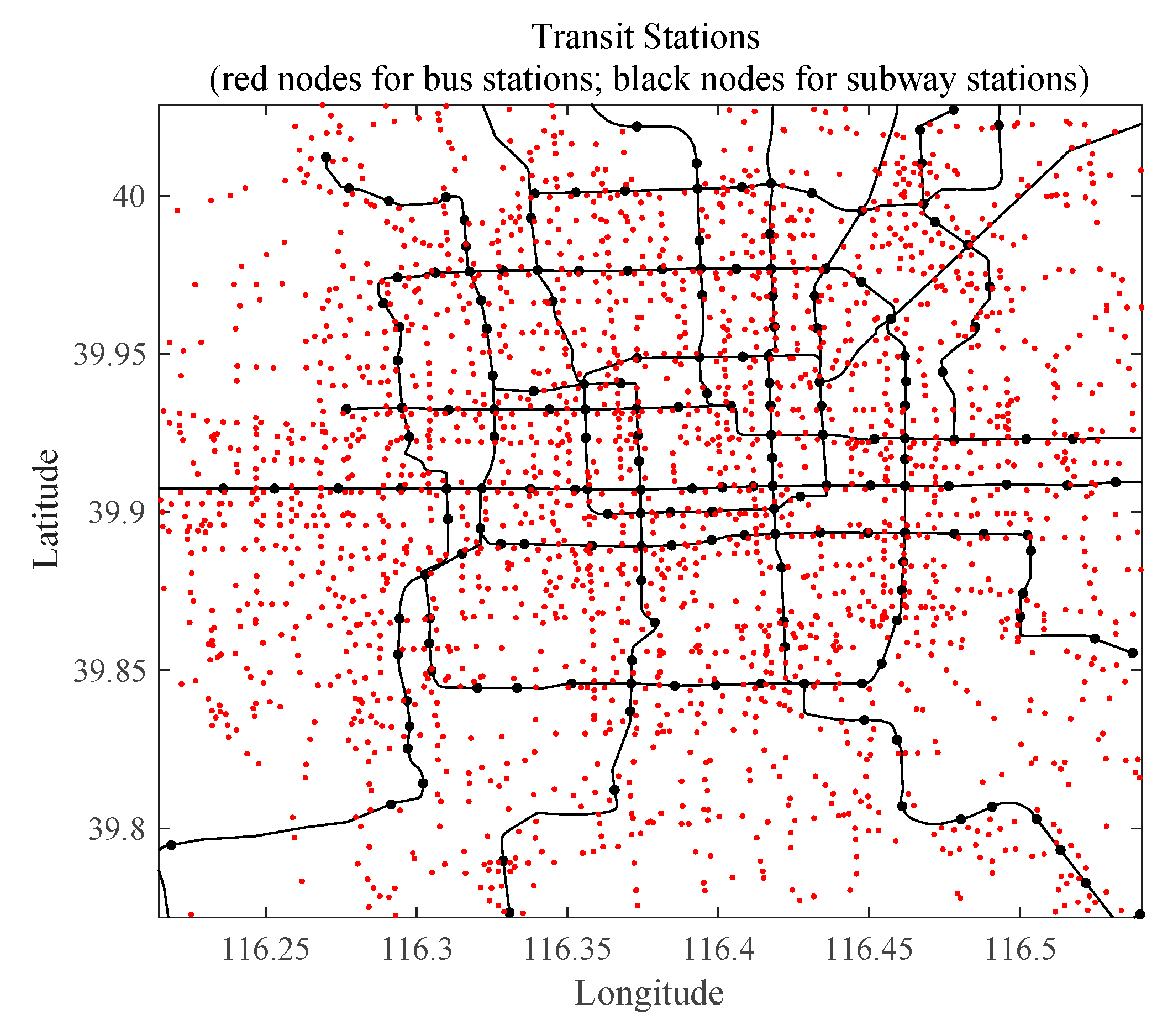
Additionally, the locations of all bus and subway stations in Beijing in August 2015 were collected (Figure 3). These transit stations’ locations were obtained from Amap (see https://lbs.amap.com). This data included the station name, line name, and longitude and latitude of the location. These data were used to analyse the relationship between the BAcc and transit stations.

3.2. Sample Formation

The process of generating the sample for numerical analysis included the following steps.

First, the weekday data were selected and pre-processed. A time series was formed for the position of each vehicle. Considering the GPS measurement error and drift, a displacement of fewer than 100 m was regarded as invalid and corrected based on the GPS positions at adjacent time points.

Second, the zones were set by dividing the study area into a grid consisting of 200 × 200 m squares, each of which was designated as a zone. A zone was the smallest unit of area used in the study, i.e., the location of a bike was taken to be a particular zone, not a specific point, and a trip was considered as going from one zone to another. Shared-bike locations were more concentrated during the daytime and more dispersed at night.

Third, using the location data, the shared-bike availability in each zone was calculated for every minute. The calculation method was as follows.

The shared-bike availability (A) is the proportion of the bicycling demand that can be served by available shared bikes over the period $\left[t, t+\mathsf{\Delta }t\right]$. The value of $\mathsf{\Delta }t$ is small enough that bicycling demand is assumed to be uniformly distributed during $\left[t, t+\mathsf{\Delta }t\right]$. The variable A is determined by $N_t,$. the number of shared bikes within a particular area at time $t$, and two kinds of activities occurring during $\left[t,t+\mathsf{\Delta }t\right]$, namely, arrivals and departures. This association can be described by the equation $A=A_n\left(N_t, CR\right)$, where $A_n$ is a function with decision variables $N_t \mathrm{and} CR$. $N_t$ is the number of shared bikes within the given area at time t. $CR$ denotes the rate of change of the number of shared bikes, which reflects departures and arrivals, and is considered to be constant during $\left[t,t+\mathsf{\Delta }t\right]$. This study assumed that there were shared bikes available when the number of shared bikes was greater than n (a number threshold) in the area. Based on the four forms of $\left(N_t, CR\right)$, the mapping relation $A_n$ is described as

$$A_n\left(N,CR\right)=\{\begin{array}{r}\hspace{1em}\hspace{1em}1,\hspace{1em} N_t\ge n and CR \ge \frac{n-N_t}{\mathsf{\Delta }t}\\ \hspace{1em}\frac{n-N_t}{\mathsf{\Delta }t·CR},\hspace{1em} N_t\ge n and CR<\frac{n-N_t}{\mathsf{\Delta }t}\\ 1-\frac{n-N_t}{\mathsf{\Delta }t·CR},\hspace{1em}{N}_t<nand CR\ge \frac{n-N_t}{\mathsf{\Delta }t}\\ \hspace{1em}\hspace{1em}0,\hspace{1em}{N}_t<nand CR<\frac{n-N_t}{\mathsf{\Delta }t}\end{array}$$

(13)

Finally, the trips by shared bike were extracted, showing there were approximately 2,300,000 trips per day in the study area.

3.3. Parameter Specification

As discussed in Section 2.1, $f_c$ is determined by $C_{private}^{day}$ and $c_{shared}$, which were set to be the same in this study as in Song et al.: $C_{private}^{day}=0.712 RMB$, which includes the purchase cost, maintenance cost, and service life, and $c_{shared}=0.5 RMB$, accounting for the preferential policies in 2015. Given this, the critical bicycling frequency ($f_c$) was calculated as 1.42 trips/day.

Additionally, the distribution of travellers’ bicycling frequency ($h\left(f\right)$) significantly impacts bicycling cost. Because the collected data set did not include the travel frequency corresponding to the travel records, a multi-scenario analysis method was adopted to set the different frequency distributions. The study by Miller and Roorda [36] was based on surveys of travel-frequency and determined that a log-normal density function represents well the travel-frequency distribution. A log-normal function ensures that the random variable is positive and close to a normal distribution. Therefore, the travellers’ bicycling frequencies in this study were assumed to follow a log-normal distribution: $lnf \sim N\left(\mu , {\sigma }^2\right)$, where the expected value of frequency $E\left(f\right)=exp\left(\mu +{\sigma }^2/2\right)$, and its variance $Var\left(f\right)=\left(exp\left({\sigma }^2\right)-1\right) · exp\left(\mu +{\sigma }^2/2\right)$. In the case study, 42 scenarios with different $E\left(f\right)$ were set within $\left(0.033, 7.000\right)$, and $Var\left(f\right)=\mathrm{0.25.}$ The 42 values of $E\left(f\right)$ within $\left(0.033, 7.000\right)$ covered travellers with bicycling frequency from one bicycling trip per 100 days to seven bicycling trips per day, which was a reasonable coverage of travellers in Beijing. Each scenario considered a group of travellers with a specified $E\left(f\right)$ and $Var\left(f\right)$.

The parameter $\alpha$ is the value of travel time to unify travel time and travel cost in Equation (1). Value of travel time is a critical indicator of individual willingness-to-pay as the implicit trade-off between time and money, which can be obtained from revealed preference (RP) data [37,38] and stated preference (SP) data [39,40]. The estimation of $\alpha$ varies widely and is generally 20~200% of the income [39]. This study set the $\alpha$ equal to the income of travellers. According to the data released by the Beijing Municipal Bureau Statistics [41], the average residents’ income in Beijing in 2017 was 29.9 RMB/h. Then $\alpha =29.9\mathrm{RMB}/\mathrm{h}$.

Equation (7) shows that $\mathsf{\Delta }BAc{c}_o/BAc{c}_o^{baseline}$ is determined by $\beta$ and $\mathsf{\Delta }{C}_{od}$. The value of $\beta$ shall be specified according to the value range of $I{M}_{od}$. In this case study, the IM values for short-distance trips were within the range [0, 30]. Testing various values of $\beta$ revealed that when the value of $\beta$ equals 0.15, IM can be well mapped to the interval [0, 1]. Therefore, for the case study, $\beta =0.15$.

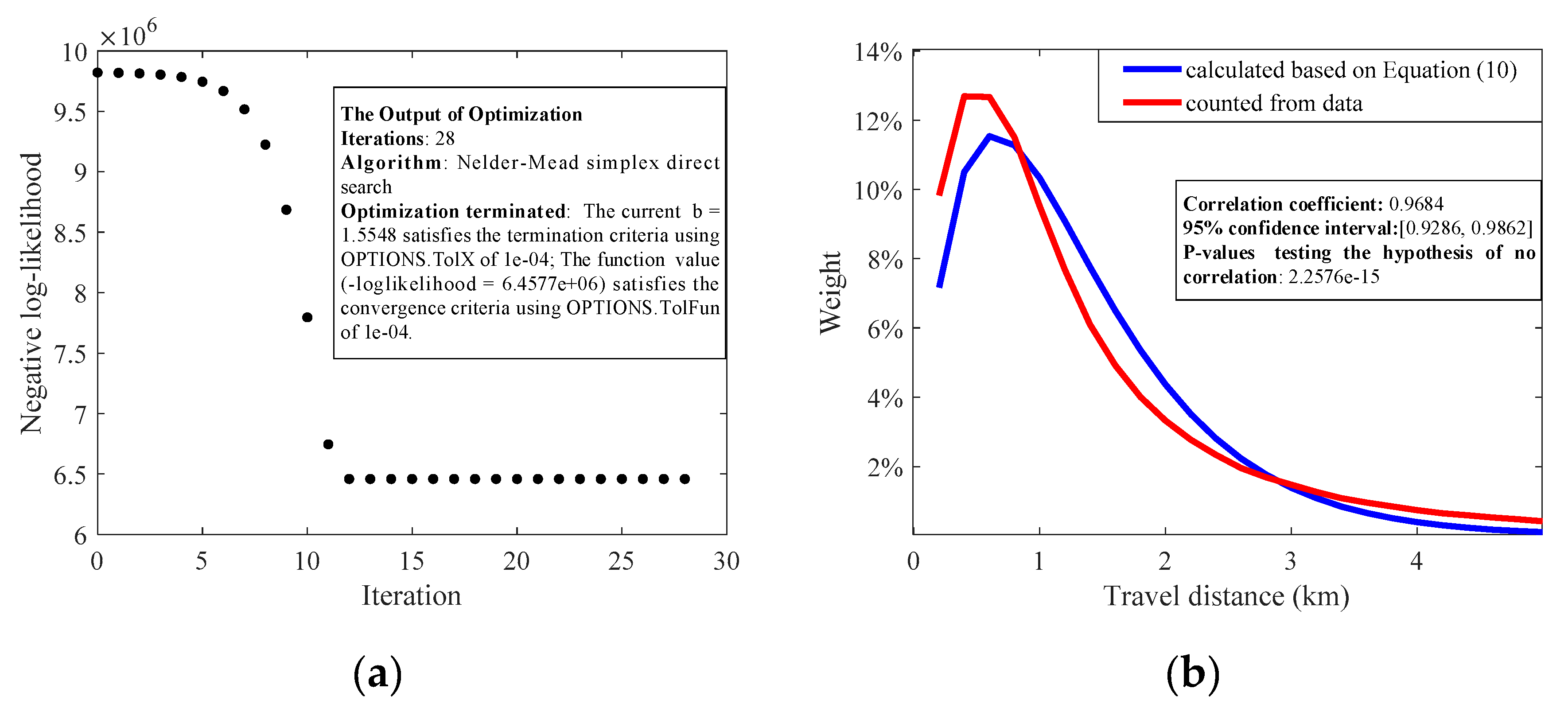
In the estimation of $W_{od}$, this study considered the number of attractions in each $200\times 200\mathrm{m}$ zone to be the same, lacking data for land use. Then the weight was not estimated based on OD pair, but based on distance. The $A{T}_d$ for each distance was viewed as the number of destination zones with this specific distance. The estimation of weight was based on the data of travelling by shared bike. This study used the log-likelihood maximization method to estimate the parameter b in Equation (10). Figure 4a plotted the optimization process. The estimated b value was 1.5548 with the stand error $7.54\times {10}^{-4}$ and a 95% confidence interval [1.5534, 1.5563], which meets the termination condition of the optimization. This case study used Manhattan distance to represent the travel distance. Since the considered area was gridded, the travel distance was discrete with the granularity being the size length of the zone (200 m). The weight of trip distribution based on the estimated parameter b was as Figure 4b.

3.4. Numerical Analysis

This section examines shared-bike availability and bicycling cost, through which bike-sharing affects the BAcc, and their characteristics in time and space. Further, improvement of BAcc in Beijing due to shared-bike availability is determined along with its characteristics in time and space.

3.4.1. Shared-Bike Availability and the Reduction of Bicycling Cost

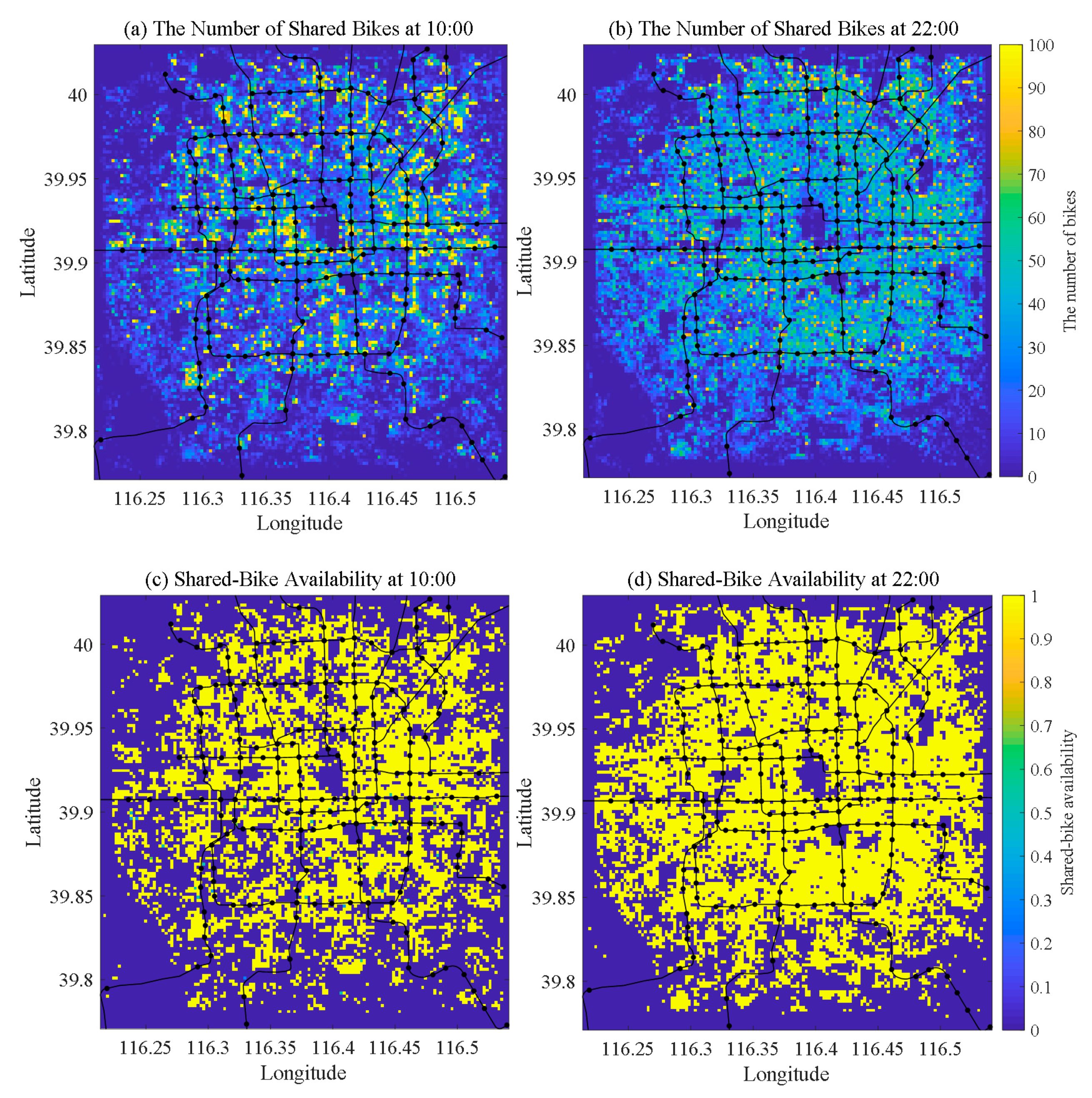
In practice, a bike-sharing system cannot guarantee that there are shared bikes available anytime and anywhere. Therefore, shared-bike availability does not always equal 1 and varies with time and space. Figure 5 shows the distribution of the shared bikes, and the calculated availability at 10 am and 10 pm. The black lines are subway lines, provided to assist with location identification. The location distribution of shared bikes was more concentrated during daytime than at night (Figure 5a,b), and the corresponding shared-bike availability was lower during the daytime than at night (Figure 5c,d)).

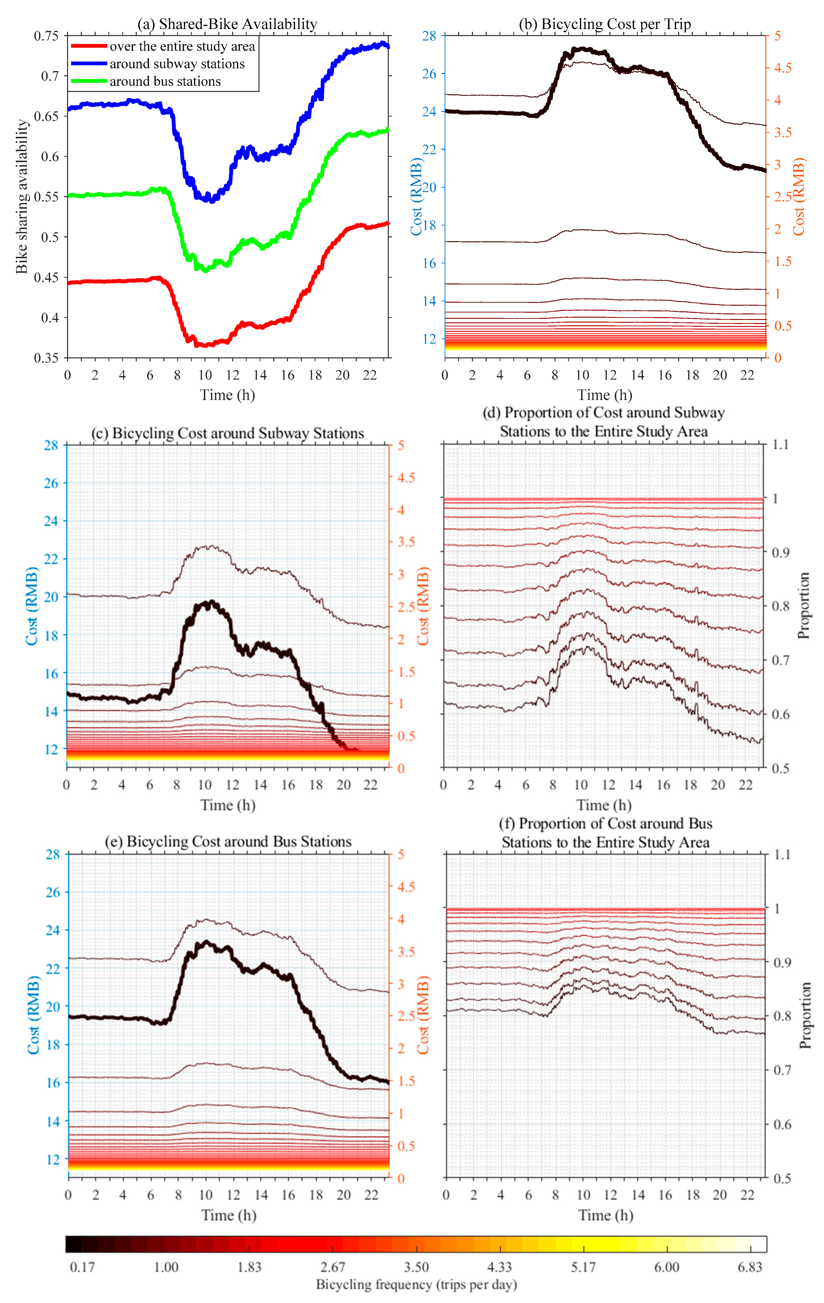
A time series of regional average values of shared-bike availability was calculated to represent its change over time more clearly. Figure 6a depicts the curves of the average values of shared-bike availability over the entire study area, around the subway stations, and around the bus stations. There are two troughs in each curve, occurring at 10 am and 2 pm. The average availability of shared bikes was lowest at 10 am. During the morning rush hour, the distribution of shared bikes changed from decentralised to concentrated, resulting in a low average availability value at the end of the morning rush hour. The trend of change in shared-bike distribution during the evening rush hour was the opposite. This dynamic distribution of shared bikes resulted in the shape of the shared-bike availability curve. In general, the average shared-bike availability calculated for the entire area was the lowest; the availability around subway stations was highest, and the availability around bus stations was between the two. The availability at night was higher than during the day because the shared bikes were more decentralised.

The variation of shared-bike availability, in turn, leads to the variation of bicycling cost. Figure 6b illustrates the overall average values of the bicycling costs in different scenarios. Two Y-axes were used to display the curves in one figure. The left Y-axis is for the thick curve with $E\left(f\right)=0.17$ times per day; the right Y-axis is for the other curves for $E\left(f\right)$ within $\left(0.17,6.83\right)$. For travelers with low bicycling frequencies, the shape of the bicycling-cost curve was opposite to the shape of the shared-bike availability curve, and the bicycling-cost curves flatten for travellers with high bicycling frequencies. For a higher bicycling frequency, the bicycling cost was less significantly affected by shared-bike availability than for a lower frequency.

The zones around the subway stations and bus stations were extracted, and the regional average of bicycling costs over these zones was examined to explore the spatial distribution characteristics of bicycling costs. The curves of the average bicycling costs around the subway and bus stations are depicted in Figure 6c,e, respectively, and the use of the double-axis and curve colours are the same as in Figure 6b. Comparing the curves in Figure 6b,c,e shows that, for people with the same bicycling frequency, the bicycling cost around transit stations was significantly lower than that over the entire study area because shared-bike availability around the transit stations was greater. In order to show the difference between the curves in Figure 6b and the curves in Figure 6c,e, Figure 6d,f show the ratio of bicycling cost around transit stations to bicycling cost over the entire study area. The lower the bicycling frequency, the lower this ratio was, indicating that travellers with a low bicycling frequency were affected more significantly. The farther the ratio was from 1, the more significant the difference between the two bicycling costs. In general, the difference was smaller in the daytime than at night and was the lowest at the end of the morning rush hour.

3.4.2. The Value of BAcc

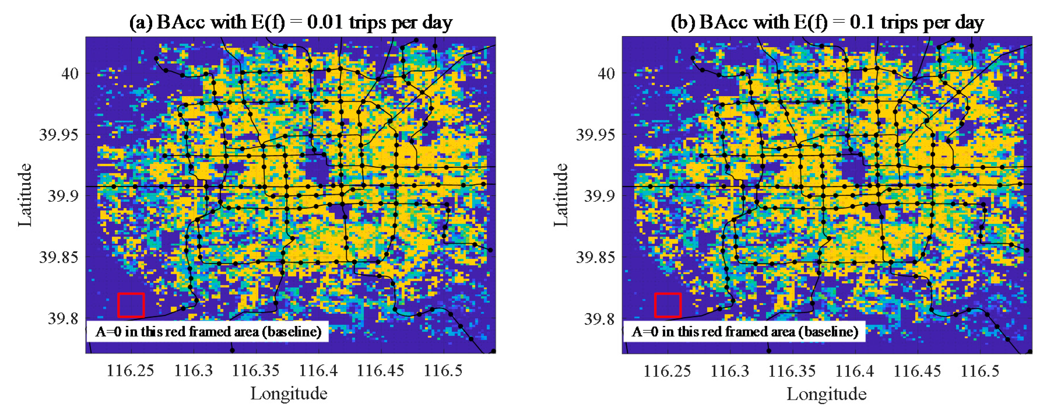
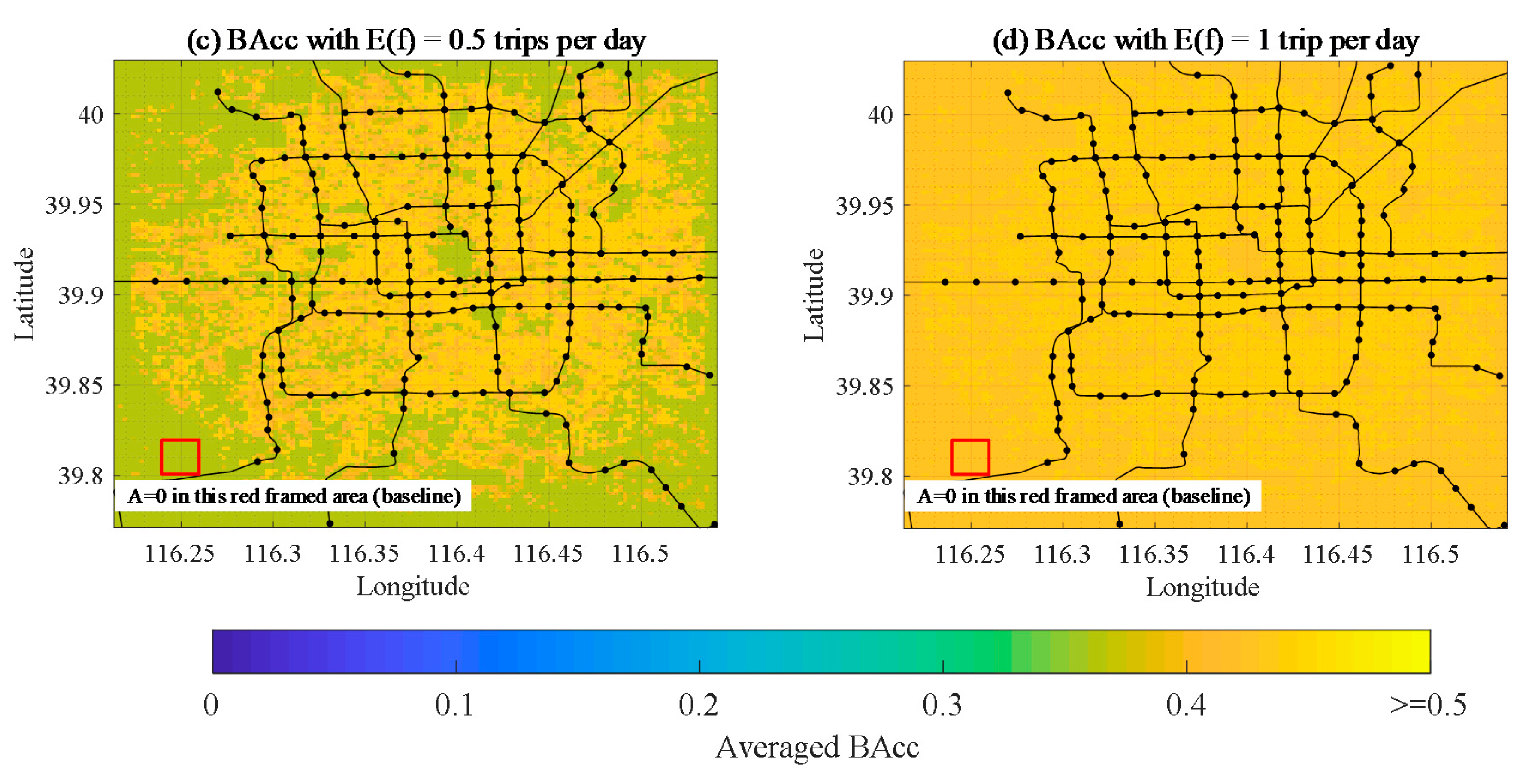
The BAcc within the considered area was calculated considering both shared bikes and private bikes. BAcc is affected by the distribution of $f$, and Figure 7 shows the BAcc under different distributions of $f$. When the expected value of $f$ is relatively low (e.g., 0.01 and 0.1 in Figure 7a,b), the BAcc value with $\mathrm{A}=0$ is close to zero, while the BAcc value with $\mathrm{A}\ne 0$ can be 0.5 or more. When the expected value of $f$ gets higher (e.g., 0.5 in Figure 7c), the BAcc value in the area with $\mathrm{A}=0$ also increases accordingly, the BAcc value in part of the area with $\mathrm{A}\ne 0$ increases, and the BAcc value in the other part of the area with $\mathrm{A}\ne 0$ stays at 0.5 or more. When the expected value of $f$ is high enough (e.g., 1 in Figure 7d), the BAcc value in the area with $\mathrm{A}=0$ is 0.51, and the maximum BAcc value in the other part of the area with $\mathrm{A}\ne 0$ is 0.53.

3.4.3. The Improvement in BAcc due to Bike-Sharing

Equations (4), (7), and (12) show that shared-bike availability leads to the reduction of bicycling cost and therefore results in increased BAcc. Based on the analysis in Section 3.4.1, this section examines the rate of increase of BAcc ($\mathsf{\Delta }BAc{c}_o/BAc{c}_o^{baseline}$). This was calculated at the locational level. Figure 8 depicts the average values of $\mathsf{\Delta }BAc{c}_o/BAc{c}_o^{baseline}$ over the entire study area (Figure 8a), and around the subway stations (Figure 8b) and bus stations (Figure 8c). Figure 8 uses a double axis, as in Figure 6, where the left Y-axis applies to the thick curve, and the right Y-axis applies to the other curves. There are three points revealed by Figure 8.

First, the rate of increase of BAcc is consistent with the availability of shared bikes. The shapes of the curves in Figure 8 are consistent with those in Figure 6a, demonstrating that the average rate of increase of BAcc was consistent with the average availability of shared bikes. This consistency increased as bicycling frequency decreased.

Second, the rate of increase of BAcc around transit stations was higher. By comparing (a), (b), and (c) in Figure 8, it can be seen that, for people with the same bicycling frequency, the rate of increase of BAcc was the greatest near the subways, followed by around the bus stations, and the lowest value was for the entire area.

Third, the impact of bike-sharing on BAcc was greatly affected by bicycling frequency. For a cyclist whose bicycling frequency was low enough, the improvement in BAcc was enormous; at 7 am, for cyclists whose bicycling frequency was 0.17 times per day, the average rate of increase in BAcc was as high as 37,000% near the subway stations, 31,000% near the bus stations, and 25,000% over the entire study area. The rate of increase in BAcc quickly decreased with increasing bicycling frequency; at 7 am, for cyclists with an expected bicycling-frequency of 0.5 times per day, the average rates of increase of BAcc were 28% near the subway stations, 24% near the bus stations, and 19% over the entire study area. In contrast, at 7 am, for a cyclist with a bicycling frequency of 1.17 times per day, the rates of increase of BAcc were 4.2% near the subway stations, 3.5% near the bus stations, and 2.8% over the entire study area. For people who bicycle more than 1.4 times per day, the improvement in bicycling accessibility was nearly zero. Therefore, it is necessary to consider bicycling frequency when measuring the impact of bike-sharing on BAcc.

4. Conclusions

In this paper, BAcc is defined as an indicator of the ease of bicycling to destinations. Shared bikes differ from private bikes in the aspect of the cost of using an available bike for a trip (bicycling cost), and herein the two types of bike were viewed as two modes for bicycling. This study investigated incorporating the impact of bike-sharing into the measurement of BAcc to make it more comprehensive. The proposed method includes a process of mode choice for the calculation of bicycling cost. When shared bikes are available, the mode with lower bicycling cost is selected, and this choice is affected by bicycling cost of the private bike, which is determined by the traveller’s bicycling frequency. The value of BAcc is determined by shared-bike availability and the distribution of bicycling frequency.

A case study of BAcc in Beijing was conducted to illustrate the significant impact of bike-sharing on BAcc and, therefore, the necessity to consider bike-sharing in its calculation. The data from Beijing showed that shared-bike availability was less during daytime than at night and reached its lowest level at the end of the morning rush hour; in terms of location, availability around the subway stations was the greatest. The spatial-temporal characteristics of the rate of increase of BAcc are consistent with those of shared-bike availability, and the lower the bicycling frequency, the greater the consistency. For low-frequency cyclists, the rate of increase of BAcc was enormous; for cyclists with a frequency of 0.17 times per day, the average BAcc at 7 am over the entire study area increased by 25,000%. However, the rate of increase of BAcc decreased quickly with increasing frequency; for those with a frequency of 0.5 times per day, the average BAcc over the entire study area increased by only 19%, and for people whose bicycling frequency was greater than 1.4 times per day, the improvement in bicycling accessibility was nearly zero.

To the best of the authors’ knowledge, this study represents the first attempt to include bike-sharing in the calculation of bicycling accessibility. For areas that have launched or are about to launch bike-sharing systems, including bike-sharing in the measurement of BAcc is necessary for evaluating both bicycling and transit accessibility. The proposed method for determining BAcc more completely measures bicycle mobility, thus improving the understanding and evaluation of bicycling conditions by decision-makers. It is noteworthy that, although the evaluation method is proposed for use in determining bicycling accessibility, it has broader applicability and could thus be extended to the measurement of accessibility by car (considering private cars, taxis, and shared cars) and other modes that involve both private and shared vehicles. Based on the limitations of the data set, land use was not considered in the numerical analysis. The proposed method only considered the private pedal bike and the shared pedal bike but did not include the private electric bike and the shared electric bike. In future studies, the measurement of bicycling accessibility can be made more comprehensive with the inclusion of land use information and considering the electric bike, and parameter $\alpha$ can be set as a dynamic parameter, varying among travellers.

References

- Martin, E.W.; Shaheen, S.A. Evaluating public transit modal shift dynamics in response to bikesharing: A tale of two US cities. J. Transp. Geogr. 2014, 41, 315–324. [Google Scholar] [CrossRef] [Green Version]
- Biking Provides a Critical Lifeline During the Coronavirus Crisis. Available online: https://www.wri.org/blog/2020/04/coronavirus-biking-critical-in-cities (accessed on 17 April 2020).
- UN Eyes Bicycles as Driver of Post-COVID-19 ‘Green Recovery’. Available online: https://www.un.org/en/coronavirus/un-eyes-bicycles-driver-post-covid-19-%E2%80%98green-recovery%E2%80%99 (accessed on 22 May 2020).
- Ben-Akiva, M.; Lerman, S. Disaggregate Travel and mobility choice models and measures of accessibility. In Behavioural Travel Modelling; Hensher, D., Stopher, P., Eds.; Croom Helm: London, UK, 1979; pp. 654–679. [Google Scholar]
- McNeil, N. Bikeability and the Twenty-Minute Neighborhood: How Infrastructure and Destinations Influence Bicycle Accessibility; Portland State University: Portland, Oregon, 2010; Available online: http://www.reconnectingamerica.org/assets/Uploads/2010mcneilbikeabilityjune2010.pdf (accessed on 4 June 2010).
- Lowry, M.B.; Furth, P.; Hadden-Loh, T. Prioritizing new bicycle facilities to improve low-stress network connectivity. Transp. Res. Part A Policy Pract. 2016, 86, 124–140. [Google Scholar] [CrossRef]
- Grigore, E.; Garrick, N.; Fuhrer, R.; Axhausen, I.K.W. Bikeability in Basel. Transp. Res. Rec. 2019, 2673, 607–617. [Google Scholar] [CrossRef]
- Krizek, K.J.; Stonebraker, E.W. Assessing options to enhance bicycle and transit integration. Transp. Res. Rec. 2011, 2217, 162–167. [Google Scholar] [CrossRef]
- Zuo, T.; Wei, H.; Rohne, A. Determining transit service coverage by non-motorized accessibility to transit: Case study of applying GPS data in Cincinnati metropolitan area. J. Transp. Geogr. 2018, 67, 1–11. [Google Scholar] [CrossRef]
- Zuo, T.; Wei, H.; Chen, N.; Zhang, C. First-and-last mile solution via bicycling to improving transit accessibility and advancing transportation equity. Cities 2020, 99, 102614. [Google Scholar] [CrossRef]
- Shaheen, S.; Chan, N. Mobility and the sharing economy: Potential to facilitate the first-and last-mile public transit connections. Built Environ. 2016, 42, 573–588. [Google Scholar] [CrossRef]
- Meituan Bicycle’s Big Data Shows Recovery from COVID-19 Stagnancy. Available online: https://pandaily.com/meituan-bicycles-big-data-shows-recovery-from-covid-19-stagnancy (accessed on 4 March 2020).
- Hansen, W.G. How accessibility shapes land use. J. Am. Inst. Plan. 1959, 25, 73–76. [Google Scholar] [CrossRef]
- Miller, E.J. Accessibility: Measurement and application in transportation planning. Transp. Rev. 2018, 38, 551–555. [Google Scholar] [CrossRef]
- Litman, T. Measuring transportation: Traffic, mobility and accessibility. Inst. Transp. Eng. ITE J. 2003, 73, 28–32. [Google Scholar]
- Litman, T. Evaluating Accessibility for Transportation Planning; Victoria Transport Policy Institute: Victoria, BC, Canada, 2008. Available online: https://vtpi.org/access.pdf (accessed on 5 June 2020).
- Penchansky, R.; Thomas, J.W. The concept of access: Definition and relationship to consumer satisfaction. Med Care 1981, 19, 127–140. [Google Scholar] [CrossRef] [PubMed]
- Saurman, E. Improving access: Modifying Penchansky and Thomas’s theory of access. J. Health Serv. Res. Policy 2016, 21, 36–39. [Google Scholar] [CrossRef] [PubMed]
- Vale, D.S.; Saraiva, M.; Pereira, M. Active accessibility: A review of operational measures of walking and cycling accessibility. J. Transp. Land Use 2016, 9, 209–235. [Google Scholar] [CrossRef]
- Handy, S.L.; Niemeier, D.A. Measuring accessibility: An exploration of issues and alternatives. Environ. Plan. A 1997, 29, 1175–1194. [Google Scholar] [CrossRef]
- Kabra, A.; Belavina, E.; Girotra, K. Bike-share systems: Accessibility and availability. Manag. Sci. 2019. [Google Scholar] [CrossRef]
- Lee, C.; Moudon, A.V. Physical activity and environment research in the health field: Implications for urban and transportation planning practice and research. J. Plan. Lit. 2004, 19, 147–181. [Google Scholar] [CrossRef]
- Moudon, A.V.; Lee, C. Walking and bicycling: An evaluation of environmental audit instruments. Am. J. Health Promot. 2003, 18, 21–37. [Google Scholar] [CrossRef]
- Winters, M.; Brauer, M.; Setton, E.M.; Teschke, K. Mapping bikeability: A spatial tool to support sustainable travel. Environ. Plan. B Plan. Des. 2013, 40, 865–883. [Google Scholar] [CrossRef]
- Cherry, C. Electric Bike Use in China and Their Impacts on the Environment, Safety, Mobility and Accessibility. UC Berkeley: Center for Future Urban Transport: A Volvo Center of Excellence. 2007. Available online: https://escholarship.org/uc/item/8bn7v9jm (accessed on 1 April 2007).
- Ding, C.; Cao, X.; Dong, M.; Zhang, Y.; Yang, J. Non-linear relationships between built environment characteristics and electric-bike ownership in Zhongshan, China. Transp. Res. Part D Transp. Environ. 2019, 75, 286–296. [Google Scholar] [CrossRef]
- Song, M.; Zhang, Y.; Shen, Z.M.; Li, M.; Dong, Z. Mode Shift from Car to Bike Shared: A Travel-Mode Choice Model. In Proceedings of the 19th COTA International Conference of Transportation Professionals, Nanjing, China, 6–8 July 2019; pp. 2398–2410. [Google Scholar]
- Van Wee, B. Accessible accessibility research challenges. J. Transp. Geogr. 2016, 51, 9–16. [Google Scholar] [CrossRef]
- Geurs, K.T.; Östh, J. Advances in the measurement of transport impedance in accessibility modelling. Eur. J. Transp. Infrastruct. Res. 2016, 16. [Google Scholar] [CrossRef]
- Fotheringham, A.S.; O’Kelly, M.E. Spatial Interaction Models: Formulations and Applications; Kluwer Academic Publishers: Dordrecht, The Netherlands, 1989; Volume 1, p. 989. [Google Scholar]
- Chillón, P.; Molina-García, J.; Castillo, I.; Queralt, A. What distance do university students walk and bike daily to class in Spain. J. Transp. Health 2016, 3, 315–320. [Google Scholar] [CrossRef]
- Sun, B.; Ermagun, A.; Dan, B. Built environmental impacts on commuting mode choice and distance: Evidence from Shanghai. Transp. Res. Part D Transp. Environ. 2017, 52, 441–453. [Google Scholar] [CrossRef]
- Zhang, Y.; Mi, Z. Environmental benefits of bike sharing: A big data-based analysis. Appl. Energy 2018, 220, 296–301. [Google Scholar] [CrossRef]
- Ben-Akiba, M.; Gunn, H.F.; Silman, L.A. Disaggregate trip distribution models. Doboku Gakkai Ronbunshu 1984, 347, 1–17. [Google Scholar] [CrossRef]
- Clifton, K.J.; Singleton, P.A.; Muhs, C.D.; Schneider, R.J. Development of destination choice models for pedestrian travel. Transp. Res. Part A Policy Pract. 2016, 94, 255–265. [Google Scholar] [CrossRef]
- Miller, E.J.; Roorda, M.J. Prototype model of household activity-travel scheduling. Transp. Res. Rec. 2003, 1831, 114–121. [Google Scholar] [CrossRef]
- Mackie, P.J.; Jara-Dıaz, S.; Fowkes, A. The value of travel time savings in evaluation. Transp. Res. Part E Logist. Transp. Rev. 2001, 37, 91–106. [Google Scholar] [CrossRef]
- Hess, S.; Bierlaire, M.; Polak, J.W. Estimation of value of travel-time savings using mixed logit models. Transp. Res. Part A Policy Pract. 2005, 39, 221–236. [Google Scholar] [CrossRef] [Green Version]
- Small, K.A. Valuation of travel time. Econ. Transp. 2012, 1, 2–14. [Google Scholar] [CrossRef]
- Liu, Y.; Gu, T.; Zhou, L.; Sun, M. SP Survey Design Based on Travel Time Value of Residents. Urban Transp. China 2018, 16, 76–82. [Google Scholar]
- Beijing Municipal Bureau Statistics. Sharing the Fruits of Economic Development, Residents’ Income Has Grown Steadily. Available online: http://tjj.beijing.gov.cn/zt/dgsdzxp/msgs/201811/t20181105_146334.html (accessed on 11 November 2018).
Figure 1.
Travel cost per trip by shared bike vs. travel cost per trip by private bike (adapted from Song et al. [27]).
Figure 2.
Process for determining the lower-cost mode.
Figure 3.
Transit stations in the study area.
Figure 4.
Estimation results. (a) Estimation of parameter b; (b) Estimation of weight.
Figure 5.
Shared-bike availability in Beijing.
Figure 6.
Shared-bike availability and bicycling cost in Beijing (the legend for bicycling frequency shown at the bottom applies to all figures).
Figure 7.
Averaged bicycling accessibility (BAcc) in Beijing.
Figure 8.
Rate of increase of BAcc in Beijing (the legend for bicycling frequency shown at the bottom applies to all figures).
© 2020 by the authors. Licensee MDPI, Basel, Switzerland. This article is an open access article distributed under the terms and conditions of the Creative Commons Attribution (CC BY) license (http://creativecommons.org/licenses/by/4.0/).
Share and Cite
MDPI and ACS Style
Song, M.; Wang, K.; Zhang, Y.; Li, M.; Qi, H.; Zhang, Y. Impact Evaluation of Bike-Sharing on Bicycling Accessibility. Sustainability 2020, 12, 6124. https://0-doi-org.brum.beds.ac.uk/10.3390/su12156124
AMA Style
Song M, Wang K, Zhang Y, Li M, Qi H, Zhang Y. Impact Evaluation of Bike-Sharing on Bicycling Accessibility. Sustainability. 2020; 12(15):6124. https://0-doi-org.brum.beds.ac.uk/10.3390/su12156124
Chicago/Turabian StyleSong, Mingzhu, Kaiping Wang, Yi Zhang, Meng Li, He Qi, and Yi Zhang. 2020. "Impact Evaluation of Bike-Sharing on Bicycling Accessibility" Sustainability 12, no. 15: 6124. https://0-doi-org.brum.beds.ac.uk/10.3390/su12156124
Note that from the first issue of 2016, this journal uses article numbers instead of page numbers. See further details here.