Inequalities and the Impact of Job Insecurity on Health Indicators in the Spanish Workforce

Abstract

In a context of high job insecurity resulting from social deregulation policies, this research aims to study health and substance abuse inequalities in the workplace from a gender perspective. To this end, a transversal study was carried out based on microdata from the National Health Survey in Spain—2017, selecting the active population and calculating the prevalence of the state of health and consumption, according to socio-occupational factors (work relationship, social occupational class, time and type of working day). Odds ratios adjusted by socio-demographic variables and their 90% confidence intervals were estimated by means of binary logistic regressions stratified by sex. The results obtained showed two differentiated patterns of health and consumption. On the one hand, unemployed people and those from more vulnerable social classes showed a higher prevalence of both chronic depression and anxiety and of hypnosedative and tobacco use. On the other hand, the better positioned social classes reported greater work stress and alcohol consumption. In addition, while unemployment affected men’s health more intensely, women were more affected by the type of working day. The study can be used to design sustainable preventive occupational health policies, which should at least aim at improving the quantity and quality of employment.

1. Introduction

More than a decade has passed since the financial crisis and the stagnation of the global economy in 2008 (the great recession) began and austerity policies (the great aggression) imposed by the Troika (formed by the European Commission, the European Central Bank and the International Monetary Fund) based on a political exchange of “neoliberal intergovernmentalism” that forced the member states of the European Union with economic difficulties, especially the countries of the South (Spain, Greece and Portugal), to deregulate the labor market and labor relations [1,2] with the “conditionality” of obtaining financial aid and bank bailouts [3]. These policies have led to a radical transformation of industrial relations models and the breakdown of the fragile balances achieved during decades of social dialogue by deregulating the three historical collective mechanisms that have acted in the defense and protection of workers: protection of legality, trade union intervention and business coverage [4]. This aggression has meant a great regression that, on the one hand, has led the most disadvantaged social classes to even worse living conditions, and, on the other hand, has slipped the middle classes into economic fragility, extending economic and social vulnerability to large social strata [5].

In this regard, with regard to the extent of social and economic vulnerability in the field of health, a study by Stuckler et al. [6,7] in post-communist countries found that massive privatization programs in the health system increased short-term adult male mortality rates by 12.8% among the most disadvantaged social classes. On a national level, the impact of austerity policies on the health of the Spanish population has been the subject of numerous investigations from the public health field, concluding that the effects on the population are heterogeneous and controversial, endangering the sustainability of the national health system [8,9,10,11,12]. In particular, important differences have been identified between the Autonomous Communities in terms of the management of the economic crisis and austerity policies. While the government of the Basque Country did not implement austerity policies during the crisis, in La Rioja, Madrid and the Balearic Islands, privatization policies were implemented in the health system [8]. In addition, the study conducted by Del Pozo-Rubio et al. [10] showed how the co-payment of dependency introduced in Spain through the Resolution of 13 July 2012 meant, on the one hand, an unequal application of co-payments between the Autonomous Communities, with Andalusia, Valencia and Catalonia having the highest levels of co-payment, and, on the other hand, how the co-payment went from 20% in the national average before the reform to 53.54% after the reform. Thus, these studies would confirm both the inequalities between social classes and between the different regions of Spain. In addition, there is empirical evidence on problems of technical quality (misdiagnosis or inappropriate diagnosis) and interpersonal quality (poorer treatment and communication) in the public health system related to cuts in the health workforce, which affects the whole population, but especially people with fewer resources and immigrants [12]. These cuts and privatizations could explain how since the beginning of the economic crisis in Spain, there has been a significant slowdown in the reduction of the cancer mortality rate [11], which would be related in some way to the studies by Stuckler and others [6,7]. This context of economic crisis jeopardizes the sustainability of the welfare state, as the protection system (healthcare and social benefits) is financed in most European countries through employers’ and workers’ contributions to work performance. As a result, austerity measures reduce state revenues, which are largely dependent on full employment and decent wage policies, leading to severe cuts in public health and other social expenditures [13]. High unemployment rates in turn erode the bargaining power of workers and their class organizations, feeding back into the spiral of deregulation and deterioration of working conditions and occupational health [14].

In this context and for the purposes of this research, there has been an increase in job insecurity both in the European Union (EU) in general and in Spain in particular [15]. Job insecurity can be defined as a perceived threat to the continuity and stability of employment as currently experienced [16] or the loss of well-being resulting from job uncertainty [17]. Different domains or facets of job insecurity can be drawn from these definitions. The first would be uncertainty in a threefold dimension: (a) uncertainty about whether or not employment will eventually be lost; (b) uncertainty about when it will occur, i.e., when the job will be lost; and (c) uncertainty about the consequences of the loss of employment [18]. The second domain would be the threat, since the uncertainty of loss of employment is comparable to the severity of the threat [19]. That is, depending on the possibilities of finding new employment and the degree of dependence on wages for survival, the degree of threat will be greater or lesser, and therefore, is related to some theories of human needs (for example, Maslow’s pyramid) [20]. Finally, there is a third dimension that refers to the powerlessness or absence of strategies available to workers to resist the threat of dismissal [21,22,23]. Thus, the lack of protection (trade unions, working without a contract, unemployment benefit systems, and so on) makes it more or less likely that they will resist the threat of unemployment [22]. In the scientific literature, various ways can be found to study and make job insecurity operational in order to measure it. On the one hand, there are studies that focus on the analysis of perceived or subjective insecurity [24], understood as an interpretation or evaluation by the worker of a series of external signs that have to do with job continuity [25]. On the other hand, there are studies that focus on the analysis of attributed insecurity [26], that is, on the objective signs of insecurity (contractual situation, position of the worker in the company, working conditions, etc.) that do not depend on the worker’s perception [24]. Although there are various ways of studying job insecurity, the fact is that perceived or subjective insecurity and attributed or objective insecurity are related, insofar as, although perceived insecurity depends on personal and contextual factors, which may lead some workers to overestimate the probability of losing their jobs, the fact is that there is empirical evidence that correlates the subjective dimension with the objective one [27]. In fact, it has been shown that temporary contracts are associated with greater self-perceived insecurity [28,29,30] and the transformation of temporary contracts into permanent contracts with a greater perception of security [31]. The focus of this research is on attributed insecurity and therefore requires further analysis. In this regard, the previous literature has identified four types of studies related to objective insecurity: (a) research that focuses on studying insecurity dynamically through unstable employment trajectories [32,33]; (b) insecurity produced by closures, restructuring or downsizing, including those workers not affected by layoffs [34,35]; (c) job insecurity from the point of view of the type of contract or contractual relationship (temporary or permanent) [36,37]; and (d) research that studies job insecurity from a multidimensional point of view not only based on the contractual relationship but also including other elements such as occupational social class or working time, approaching the concept of job insecurity [38,39,40,41]. From the classification given, this study is part of the proposals for measuring insecurity attributed from a multidimensional perspective. It should be noted that this holistic perspective is related to labor precariousness, since this construct is broader and contemplates insecurity but not in an isolated manner [25].

Focusing on the health effects of perceived job insecurity, previous studies have identified how a subjective perception of insecurity leads to an erosion of job satisfaction [42], increased feelings of anxiety [15], or high levels of stress comparable to those who are unemployed [16]. However, the psychological health effects of job insecurity can be modulated by subjective employability [43]. In other words, subjective employability differs from objective employability (observable contextual conditions such as contractual conditions [44]) because it focuses on people’s belief that they can easily find a new job based on their genuine skills, such as work experience or educational level [45], and that previous studies have shown that it is associated with lower levels of psychological risk when unemployment is addressed proactively [45,46,47].

With regard to the health effects of attributed or objective job insecurity, it has been shown that unemployment exposes individuals to greater psychological risk [48,49]. Specifically, unemployment has been associated with a worse self-perceived general health status [50], increased mental illness such as anxiety and depression [51,52], psychosomatic and sleep disorders [43,49], the use of hypnosedatives [50,53], addictive behaviors such as the consumption of alcohol, tobacco or drugs [50,53,54], and even family conflicts and suicides [48]. If we focus on the multidimensional perspective of this study, previous research has observed elements of job insecurity attributed to the increase in psychosomatic disorders and unhealthy habits, such as the use of hypnosedatives and addictive substances that erode people’s health [55,56,57,58,59,60]. Specifically, with regard to contractual status, working conditions and occupational social class, it has been identified that (a) people on temporary contracts use health services less frequently for fear of being absent from work and dismissed [55]; (b) working long hours has been associated with higher levels of alcohol consumption [55]; (c) night work has been associated with regular smoking [56]; (d) high levels of occupational stress have been associated with a higher prevalence of alcohol consumption [57,58] and the use of hypnosedatives [59]; and (e) the more vulnerable manual social classes have been associated with poor mental health [60] and regular tobacco use [55].

From the findings of the previous literature, it is possible to observe multiple and complex bilateral and multilateral relationships between socio-professional factors, on the one hand, and the spiral of constant health deterioration on the other. For example, work-related stress has been associated with depression or anxiety [60,61]. These mental disorders are in turn linked to the use of hypnosedatives [59] and addictive behavior [57,58]. Even among the most disadvantaged manual workers, alcohol consumption has been found to be associated with an increased likelihood of losing their job [62], which deepens the feedback between social vulnerability and health impairment.

Given the complexity and current occupational vulnerability in Spain and the scarce specific and partial studies that study the associations between mental health, the use of hypnosedatives and the consumption of addictive substances in the workplace, it is necessary to carry out more extensive analyses to explore possible patterns of relationships between all the aforementioned variables of health and consumption of the active population in the labor market, in order to establish sustainable health and employment policies that reverse the health emergency situation caused, to a certain extent, by the economic crisis management policies themselves. Therefore, the main objective of this research is to explore, holistically and jointly, the possible patterns between the main occupational factors of attributed or objective job insecurity (type of contract or employment relationship, occupational social class, working time and type of working day) and the various health factors (general and mental state, consumption of hypnosedatives, tobacco and alcohol) in the Spanish active population. In addition, several studies indicate that the different gender roles in the area of reproductive tasks [63,64] and the precarious working conditions that affect working women most intensely [65,66] make them more likely to refer to psychosomatic disorders and to consume more hypnosedatives [67,68,69]. In light of these findings, it is considered relevant to address the objective of this research to explore health and consumption patterns by stratifying the working population sample by sex.

2. Materials and Methods

2.1. Sample and Study Population

In order to achieve the proposed objectives, the use of the microdata from the questionnaire for adults from the National Health Survey (ENSE, 2017) [70], carried out by the Ministry of Health, Consumption and Social Welfare of Spain, was considered the most suitable source for carrying out the study, since for each Autonomous Community, an independent sample was designed, which allowed for having a large and representative sample of the entire country [71]. The sample carried out was a polytopic one. In the first stage the census sections were selected and in the second stage the main family dwellings were selected. In each dwelling, an adult person aged 16 years old or over was selected to carry out the adult questionnaire. The fieldwork was extended between the months of October 2016 and October 2017, for the purpose of collecting data that might be affected by seasonality. The total size of the ENSE survey for adults in 2017 was 23,089 persons, with a high response rate of 95%. Information was collected through personal interviews. The same was complemented, in exceptional cases, by means of a telephone interview. For the present study, only the active population was selected. The active population was considered to be those persons who were of working age (16 years old or over in Spanish legislation) and who carried out a professional activity, as well as those persons of working age who were unemployed and who were actively seeking employment [72]. Thus, the sample for this research was 12,260 persons between the ages of 16 and 64 years old. Specifically, the study included a sample of 6299 men (5163 (82%) employed and 1136 (18%) unemployed) and 5931 women (4610 (77.3%) employed and 1351 (22.7%) unemployed) (

Table 1. Sociodemographic characteristics of the active population in Spain, health status, consumption of hypnosedatives, tobacco and alcohol, according to sex.

Variables	Men (n = 6299; 51.4%)	Women (n = 5961; 48.6%)	p-Value b
	n (%) a	n (%) a
Self-perceived health status			<0.001
Bad	1168 (18.5)	1486 (24.9)
Good	5131 (81.5)	4475 (75.1)
Visits to the family doctor			<0.001
No	1902 (30.2)	1069 (17.9)
Yes	4397 (69.8)	4892 (82.1)
Depression			<0.001
No	6012 (95.5)	5391 (90.4)
Yes	285 (4.5)	566 (9.5)
DK/DA	2 (0.0)	4 (0.1)
Chronic anxiety			<0.001
No	5960 (94.6)	5302 (89.0)
Yes	334 (5.3)	651 (10.9)
DK/DA	5 (0.1)	8 (0.1)
Stress			<0.001
No	2670 (51.7)	2209 (48.1)
Yes	2484 (48.1)	2388 (51.8)
DK/DA	9 (0.2)	3 (0.1)
Tranquilizers, relaxants, sleeping pills			<0.001
No	2840 (45.0)	3137 (52.6)
Yes	369 (5.9)	601 (10.1)
DK/DA	3090 (49.1)	2223 (37.3)
Antidepressants, stimulants			<0.001
No	3072 (48.7)	3431 (57.6)
Yes	137 (2.2)	307 (5.1)
DK/DA	3090 (49.1)	2223 (37.3)
Smoke			<0.001
No	4148 (65.9)	4205 (70.6)
Yes	2144 (34.1)	1753 (29.4)
DK/DA	7 (0.1)	3 (0.0)
Alcohol			<0.001
No	2102 (33.4)	3384 (56.8)
Yes	4192 (66.6)	2573 (43.2)
DK/DA	5 (0.1)	4 (0.1)
Type of contract or employment situation			<0.001
Entrepreneur	370 (5.9)	182 (3.1)
Official	505 (8.0)	607 (10.2)
Indefinite salaried	2754 (43.7)	2517 (42.2)
Temporary employee	769 (12.2)	788 (13.2)
Autonomous	742 (11.8)	460 (7.7)
Without contract	23 (0.4)	56 (0.9)
Unemployed	1136 (18%)	1351 (22.7)
Occupational Category			<0.001
Managers with more than 10 workers	732 (11.6)	759 (12.8)
Managers with fewer than 10 workers	525 (8.3)	584 (9.8)
Intermediate technicians	1190 (18.9)	1270 (21.4)
Qualified supervisors	957 (15.2)	582 (9.8)
Qualified manual technicians	2045 (32.5)	1808 (30.3)
Unqualified manual technicians	809 (12.8)	924 (15.5)
DK/DA	41 (0.7)	34 (0.6)
Working time			<0.001
Full time	4894 (94.8)	3616 (78.5)
Part time	268 (5.2)	987 (21.4)
DK/DA	1 (0.0)	7 (0.1)
Type of working day			<0.001
Split shift	2105 (40.8)	1379 (29.9)
Continue in the morning	1383 (26.8)	1638 (35.9)
Continue in the afternoon	117 (2.3)	201 (4.4)
Continue through the night	68 (1.3)	37 (0.8)
Shifts	39 (0.8)	183 (4)
Irregular or variable day according to the days	757 (14.8)	616 (13.4)
Other types	637 (12.5)	506 (10.9)
DK/DA	57 (1.1)	50 (1.0)
Age			0.006
16–24	230 (3.7)	200 (3.4)
25–34	946 (15.0)	1022 (17.1)
35–44	1924 (30.5)	1844 (30.9)
45–54	1851 (29.4)	1851 (29.0)
≥55	1348 (21.4)	1168 (19.6)
Nationality			0.014
Spanish	5516 (87.6)	5131 (86.1)
Foreigner	783 (12.4)	830 (13.9)
Marital status			<0.001
Single	1937 (30.7)	1667 (28.0)
Married	3840 (61)	3310 (55.7)
Widower	54 (0.9)	181 (3.0)
Divorced	463 (7.4)	789 (13.3)
DK/DA	5 (0.1)	14 (0.2)
Education level			<0.001
Primary	860 (13.7)	604 (10.1)
Secondary	4077 (64.7)	3501 (58.7)
Tertiary	1362 (21.6)	1856 (31.1)
Type of family life			<0.001
Married	3597 (57.1)	2813 (47.2)
Domestic partner	189 (3.0)	137 (2.3)
Do not live together	2513 (39.9)	3010 (50.5)
Family care work			<0.001
No	5706 (90.6)	5216 (87.5)
Yes	592 (9.4)	745 (12.5)
Monthly household income			0.781
Less than 1050 euros per month	1983 (31.5)	5216 (87.5)
From 1050 to less than 2200 euros	2739 (43.5)	745 (12.5)
From 2200 to less than 4500 euros	1540 (24.4)	1465 (24.6)
More than 4500 euros per month	37 (0.6)	26 (0.5)

^an = number; % =percentage of total sample; ^b p value = sex differences calculated using Chi-square test, with 95% confidence level. DK/DA= Does not know/does not answer.

).

2.2. Dependent, Independent and Covariant Adjustment Variables

Nine dichotomised dependent variables were used. The general health status was evaluated on the basis of two questions: (a) “In the last twelve months, would you say your health status has been very good, good, fair, bad, very bad?” This question was dichotomized into 0 = Bad health (fair/bad/very bad) and 1 = Good health (very good/good); and (b) “When was the last time you consulted your general practitioner or family doctor for yourself?” The variable was dichotomized into 0 = No (12 months ago or more/Never) and 1 = Yes (Within the last 4 weeks/Between 4 weeks and 12 months). It is worth mentioning that the self-perceived health variable was dichotomized following common practices in public health studies [73,74,75]. In addition, we studied the relationship between the self-perceived health variable constructed with twenty-five indicators of pathologies diagnosed by health professionals, finding in all cases a statistically significant relationship that shows how people with good self-perceived health present a lower frequency of being diagnosed with pathologies (

Table A1. Relationship between self-perceived health and health problems.

Pathologies	Self-Perceived Ill Health Nº (%) a	Good Self-Perceived Health Nº (%) a	p–Value b
High blood pressure	6047 (32)	313 (7.5)	0.000
Myocardial infarction	529 (2.8)	17 (0.4)	0.000
Angina pectoris	504 (2.7)	11 (0.3)	0.000
Other heart diseases	1535 (8.1)	51 (1.2)	0.000
Varicose veins in the legs	3298 (17.5)	219 (5.2)	0.000
Arthrosis	5304 (28.2)	155 (3.7)	0.000
Back pain (cervical)	4007 (21.2)	130 (3.1)	0.000
Back pain (lumbar)	5199 (27.5)	190 (4.5)	0.000
Chronic allergy	3447 (18.3)	469 (11.2)	0.000
Asthma	1280 (6.8)	139 (3.3)	0.000
Bronchitis	1152 (6.1)	34 (0.8)	0.000
Diabetes	2214 (11.7)	61 (1.5)	0.000
Stomach ulcer	1040 (5.5)	42 (1)	0.000
Urinary incontinence	1422 (7.5)	43 (1)	0.000
High cholesterol	5207 (27.6)	323 (5.8)	0.000
Cataracts	2881 (15.3)	126 (3)	0.000
Skin problems	1371 (7.3)	126 (3)	0.000
Chronic constipation	1123 (5.9)	33 (0.8)	0.000
Liver dysfunction	336 (1.8)	12 (0.3)	0.000
Ictus	498 (2.6)	10 (0.2)	0.000
Frequent headaches	2450 (13)	166 (6.3)	0.000
Hemorrhoids	1830 (9.7)	136 (3.2)	0.000
Malignant tumors	1130 (6)	53 (1.3)	0.000
Osteoporosis	1177 (6.2)	40 (1)	0.000
Thyroid problems	(1526 (8.1)	122 (2.9)	0.000
Kidney problems	1145 (6.1)	35 (0.8)	0.000

^an = Number; % = Percentage over the total sample; ^b p value = Sex differences calculated using a chi-squared test, with 95% confidence level.

, Appendix A) and, therefore, demonstrate the validity of the constructed variable.

With regard to the state of mental health, three variables were used. Two of them refer to whether the person interviewed suffered from depression in the last 12 months (0 = No; 1 = Yes) or chronic anxiety (0 = No; 1 = Yes). The third variable, corresponding to work stress, was measured through the following question: “Globally and taking into account the conditions in which you carry out your work, indicate how you consider the level of stress of your work according to a scale from 1 (not at all stressful) to 7 (very stressful)”. The question was dichotomized by the median which was 4, with 0 = No (from 1 to 4) and 1 = Yes (from 5 to 7). The consumption of hypnosedatives was measured through two questions referring to whether in the last 12 months the person interviewed had consumed tranquilizers, relaxants and/or sleeping pills (0 = No; 1 = Yes), or whether he/she took antidepressants and/or stimulants (0 = No; 1 = Yes). Finally, addictive behaviors were measured through two questions: (a) “Could you tell me if you smoke?”—the question was dichotomized into 0 = No (I don’t currently smoke, but have smoked before/I don’t smoke or have never smoked regularly) and 1 = Yes (Yes, I smoke daily/I do smoke, but not daily); and (b): “During the past 12 months, how often have you had alcoholic beverages of any kind?”—it was dichotomized by the median; this resulted in 0 = No (Never/No in last 12 months/3 days per month to less than 1 day in a month) and 1 = Yes (Daily or almost daily/6 to 1 days per week).

The independent variables correspond to the main socio-labor characteristics present in the ENSE survey itself. These are: the type of contract or employment situation, the socio-labor category, the working time and the type of working day. It is worth noting that it was not necessary to transform any of the four independent variables, since the ENSE already provided them in an adequate manner to carry out the study. The socio-demographic adjustment variables were age, nationality, marital status, level of education, the income of the family household, type of family life and family care work, following the guidelines of previous studies with similar characteristics [54,56,76]. These variables were selected because they interact predictably with gender roles and can affect men and women differently and act as confounding variables [59,60,61,62]. In fact, to avoid selection problems in the female labor force, these studies incorporate family status and care work as adjustment variables, since the reproductive and productive spheres are interconnected [60]. However, in order to verify the presence or absence of selection bias in the female labor force derived from their lower level of participation in the labor market, the Heckman two-stage model was used. The results obtained (

Table A2. Relationship between self-perceived health and health problems.

Dependent Variables
Selection Regressors	Self-Perceived Health Status	Visits to the Family Doctor	Depression	Chronic Anxiety	Work Stress	TRANQUILIZERS	Antidepressants, Stimulants	Smoking	Alcohol
	Selection Variable: Labor Market Participation Reference Category = Participates
	Coefficients (Standard Errors)
Const	0.580308 *** (0.144644)	0.58030 *** (0.144644)	0.58663 *** 0.144724	0.57940 *** (0.144529)	0.55839 *** (0.149458)	−0.0696068 (0.162769)	−0.0605752 (0.163026)	0.59434 *** (0.143625)	0.5837 *** 0.144749
Age	−0.127013 *** (0.0181994)	−0.1270 *** (0.018199)	−0.1279 *** 0.0182110	−0.1232 *** (0.018443)	−0.1216 *** (0.020210)	−0.04986 ** (0.020718)	−0.0517226 ** (0.0207184)	−0.1272 *** (0.018069)	−0.1275 *** 0.0182146
Nationality	0.0539992 (0.0521977)	0.0539992 (0.052197)	0.0505017 (0.052265)	0.0388518 (0.052780)	0.0587547 (0.052681)	0.0539741 (0.057980)	0.0474748 (0.0585688)	0.032670 (0.052608)	0.0568324 0.0208021
Marital status	0.0560410 *** (0.0207951)	0.05604 *** (0.020795)	0.05636 *** 0.0207978	0.05985 *** (0.020785)	0.05703 *** (0.020811)	0.07197 *** (0.022819)	0.0745274 *** (0.0231137)	0.06513 *** (0.020811)	−0.5189 *** 0.0320898
Education level	0.168384 (0.0513444)	−0.5175 *** (0.032069)	−0.5178 *** 0.0320754	−0.5217 *** (0.032004)	−0.5183 *** (0.032044)	0.47523 *** (0.035425)	−0.472219 *** (0.0356332)	−0.5169 *** (0.032019)	−0.5189 *** 0.0320898
Type of family life	−0.095654 *** (0.0269741)	−0.0956 *** (0.026974)	−0.0960 ** 0.0269798	−0.0946 *** (0.026908)	−0.0970 0.0270509	−0.0805 *** (0.029962)	−0.0868289 *** (0.0303375)	−0.0996 *** (0.026802)	−0.0952 *** 0.0269854
Family care work	0.168384 *** (0.0513444)	0.16838 *** (0.051344)	0.16905 *** 0.0513490	0.17170 *** (0.051159)	0.16852 *** (0.051284)	0.18299 *** (0.055725)	0.186160 *** (0.0557636)	0.16628 *** (0.051045)	0.1694 *** 0.0513535
Rho	0.061416	−0.024296	0.0190499	−0.014888	0.077386	−0.026900	−0.022732	−0.024091	−0.017310

*** Significant at 99% confidence; ** Significant at 95% confidence.

) show that there is no selection bias in any of the nine dependent variables derived from the fact that the correlation coefficients of the error terms of the two equations (Rho) are close to zero and are not significant. Therefore, the likelihood test carried out to verify the null hypothesis of independence between the equations is not rejected. In addition, it can be seen how the coefficients of each variable show how women who are married or live with a partner and in households where there are care jobs have less participation in the labor market. These findings would reinforce the robustness of the results of the present study. Finally, it should be mentioned that the answers “don’t know” and “don’t respond” were eliminated from the statistical analyses.

2.3. Statistical Analysis

First, a descriptive analysis of the absolute and relative (%) frequencies of all the variables used was performed, and the differences between men and women were recorded using the chi-square test (p < 0.05) (Table 1). Secondly, before stratifying the sample by sex, in order to compare differences between health and consumption indicators between men and women, adjusted odds ratios (aOR) were calculated for all socio-labor and demographic variables and their 90% confidence intervals, using logistic regression models, establishing men as the reference category (Figure 1 and

Table 2. Regressions of health and consumption indicators with the interactions between gender with the type of work relationship and occupational social class.

	Health Status Last 12 Months		You Have Suffered from Mental Disorders in the Last 12 Months			Consumption of Sedative Hypnotics in the Last 12 Months		Use of Addictive Substances in the Last 12 Months
	Self-Perceived Health Status aOR (IC90%) a	Visits to the Family Doctor aOR (IC90%) a	Depression aOR (IC90%) a	Chronic Anxiety aOR (IC90%) a	Work Stress aOR (IC90%) a	Tranquilizers aOR (IC90%) a	Antidepressants, Stimulants aOR (IC90%) a	Smoking aOR (IC90%) a	Alcohol aOR (IC90%) a
Entrepreneurs	1 b	1 b	1 b	1 b	1 b	1 b	1 b	1 b	1 b
Officials	1.57 (1.27–1.90) g	0.58 (0.4–0.69) g	1.44 (1.06–1.9) f	1.68 (1.28–2.2) g	1.04 (0.90–1.21)	1.52 (1.17–1.9) g	1.67 (1.14–2.44) f	0.70 (0.59–0.83) g	0.41 (0.3–0.47) g
Indefinite wage earners	1.72 (1.55–1.90) g	0.53 (0.4–0.58) g	1.78 (1.52–2.0) g	1.85 (1.59–2.1) g	1.30 (1.19–1.4) g	1.36 (1.17–1.58) g	1.46 (1.16–1.84) g	0.84 (0.77–0.92) g	0.40 (0.3–0.44) g
Temporary employees	1.54 (1.30–1.83) g	0.54 (0.4–0.63) g	2.33 (1.84–2.9) g	1.94 (1.65–2.4) g	0.80 (0.7–0.91) f	1.06 (0.81–1.39)	2.06 (1.48–2.89) g	0.86 (0.75–0.98) e	0.39 (0.3–0.45) g
Freelancers	1.65 (1.40–1.96) g	0.39 (0.3–0.45) g	1.70 (1.27–2.33) g	1.57 (1.17–2.1) g	0.96 (0.81–1.12)	1.42 (1.06–1.89) f	1.58 (1.05–2.3) f	0.67 (0.55–0.81) g	0.39 (0.3–0.46) g
Without contract	1.85 (0.73–4.66)	0.49 (0.24–1.06)	4.03 (2.22–7.3) g	3.96 (2.2–7.0) g	0.58 (0.3–0.95) e	1.71 (0.87–3.41)	4.01 (1.92–8.3) g	0.35 (0.20–0.64) g	0.26 (0.1–0.44) g
Unemployed	1.03 (0.91–1.17)	0.56 (0.49–0.64) g	3.19 (2.71–3.2) g	3.15 (2.69–3.6) g	- d	1.96 (1.65–2.31) g	2.95 (2.36–3.69) g	0.89 (0.79–0.99) e	0.27 (0.2–0.30) g
Managers with more than 10 employees	1 b	1 b	1 b	1 b	1 b	1 b	1 b	1 b	1 b
Managers with fewer than 10 employees	0.97 (0.84–1.12)	1.34 (1.16–1.5) g	1.48 (1.2–1.82) g	1.42 (1.15–1.7) g	0.90 (0.76–1.05)	1.38 (1.14–1.67) f	1.72 (1.33–2.22) g	0.70 (0.61–0.81) g	0.50 (0.4–0.56) g
Intermediate technicians	0.81 (0.74–0.88) g	1.69 (1.51–1.8) g	1.74 (1.5–1.97) g	1.97 (1.74–2.2) g	1.14 (1.02–1.2) e	1.68 (1.50–1.88) g	1.72 (1.47–2.02) g	0.75 (0.69–0.82) g	0.44 (0.4–0.48) g
Qualified supervisors	0.68 (0.62–0.75) g	2.32 (2.0–2.69) g	2.03 (1.7–2.32) g	2.23 (1.94–2.5) g	0.86 (0.74–1.02)	2.01 (1.78–2.27) g	2.02 (1.71–2.39) g	0.70 (0.63–0.79) g	0.29 (0.2–0.32) g
Qualified manual technicians	0.64 (0.60–0.69) g	1.99 (1.81–2.1) g	2.45 (2.23–2.6) g	2.27 (2.05–2.5) g	1.14 (1.03–1.2) e	1.95 (1.78–2.13) g	2.29 (2.03–2.59) g	0.75 (0.69–0.80) g	0.28 (0.2–0.30) g
Unqualified manual technicians	0.59 (0.54–0.65) g	2.18 (1.91–2.5) g	2.43 (2.1–2.73) g	2.45 (2.16–2.7) g	0.91 (0.79–1.06)	1.95 (1.74–2.18) g	2.22 (1.90–2.59) g	0.72 (0.65–0.80) g	0.24 (0.2–0.26) g

^a OR: odds ratio adjusted for the four socio-labor variables included in the table (type of contract or employment situation, occupational category, working time and type of working day) and the demographic variables (age, nationality, marital status, level of education, type of family life, family care work, monthly household income); IC 90%: confidence interval; ^b Reference category. In interactions the reference category is men; ^c Insufficient sample size for analysis; ^d Indicators measured only in employed persons; ^e Significance level value of p < 0.1; ^f Significance level value of p < 0.05; ^g Significance level value of p < 0.01.

). Third, once the comparison between both sexes was made, the sample was stratified between the male and female labor force to find associations between socio-labor factors and health and consumption indicators. To this end, as in the previous case, logistical regressions adjusted for all socio-labor and demographic variables were carried out for both the male (

Table 3. Adjusted logistic regression between socio-labor determinants and health and consumption indicators in the male labor force.

	Health Status Last 12 Months		You Have Suffered from Mental Disorders in the Last 12 Months			Consumption of Sedative-Hypnotics in the Last 12 Months		Use of Addictive Substances in the last 12 Months
	Self-Perceived Health Status aOR (IC90%) a	Visits to the Family Doctor aOR (IC90%) a	Depression aOR (IC90%) a	Chronic Anxiety aOR (IC90%) a	Work Stress aOR (IC90%) a	Tranquilizers aOR (IC90%) a	Antidepressants, Stimulants aOR (IC90%) a	Smoke aOR (IC90%) a	Alcohol aOR (IC90%) a
Entrepreneurs	1 b	1 b	1 b	1 b	1 b	1 b	1 b	1 b	1 b
Officials	1.04 (0.77–1.41)	1.04 (0.81–1.34)	1.67 (0.87–3.21)	1.84 (0.97–3.47)	0.60 (0.47–0.7) g	1.60 (0.96–2.66)	3.33 (1.11–9.91)	0.71 (0.55–0.92) f	0.85 (0.66–1.11)
Indefinite wage earners	1.07 (0.84–1.36)	1.01 (0.84–1.26)	1.01 (0.57–1.77)	1.57 (0.90–2.73)	0.78 (0.6–0.94) f	1.13 (0.73–1.74)	1.85 (0.68–5.03)	0.94 (0.77–1.16)	0.86 (0.69–1.05)
Temporary employees	0.91 (0.69–1.21)	1.13 (0.89–1.44)	1.52 (0.81–2.87)	1.63 (0.88–3.03)	0.55 (0.4–0.68) g	0.89 (0.53–1.52)	3.43 (1.19–9.93) f	1.27 (1.01–1.60) f	0.81 (0.64–1.03)
Freelancers	1.04 (0.79–1.36)	0.75 (0.59–0.9) e	1.18 (0.63–2.22)	1.83 (1.01–3.3) e	0.47 (0.2–1.03)	0.92 (0.55–1.53)	2.67 (0.93–7.67)	0.91 (0.77–1.14)	0.92 (0.73–1.17)
Without contract	1.07 (0.41–2.79)	1.07 (0.49–2.33)	3.44 (0.87–13.5)	- c	0.64 (0.5–0.79) f	- c	5.53 (0.75–40.74)	1.59 (0.77–3.31)	0.56 (0.27–1.16)
Unemployed	0.57 (0.38–0.89) g	1.15 (0.83–1.60)	5.53 (2.4–12.2) g	5.92 (2.8–12,4) g	- d	3.09 (1.60–5.95) g	6.75 (1.91–23.83) g	1.75 (1.28–2.41) g	0.51 (0.3–0.71) g
Managers with more than 10 employees	1 b	1 b	1 b	1 b	1 b	1 b	1 b	1 b	1 b
Managers with fewer than 10 employees	0.89 (0.73–1.10)	1.27 (1.06–1.5) e	1.54 (0.98–2.31)	1.44 (0.98–2.11)	0.89 (0.73–1.09)	1.63 (1.21–2.20) f	1.43 (0.83–2.48)	1.36 (1.12–1.64) g	0.93 (0.78–1.10)
Intermediate technicians	0.80 (0.67–1.00)	1.24 (1.06–1.4) e	2.10 (1.5–2.95) g	1.60 (1.16–2.2) f	0.87 (0.74–1.04)	1.34 (1.0–1.79)	1.75 (1.11–2.75) e	1.41 (1.20–1.66) g	0.87 (0.75–1.05)
Qualified supervisors	0.76 (0.64–0.91) f	1.39 (1.18–1.6) e	1.78 (1.25–2.5) f	1.59 (1.13–2.2) f	0.84 (0.69–1.02)	1.48 (1.13–1.94) f	1.89 (1.19–3.01) f	1.81 (1.53–2.14) g	1.01 (0.86–1.17)
Qualified manual technicians	0.69 (0.58–0.82) g	1.24 (0.99–1.65)	2.22 (1.58–3.1) g	1.76 (1.27–2.4) g	0.63 (0.5–0.76) g	1.36 (1.00–1.77)	1.77 (1.13–2.77) f	2.07 (1.76–2.42) g	0.88 (0.76–1.01)
Unqualified manual technicians	0.57 (0.48–0.69) g	1.20 (0.96-1.44)	2.39 (1.67–3.4) g	2.40 (1.71–3.4) g	0.51 (0.40–0.6) g	1.92 (1.44–2.56) g	2.30 (1.42–3.71) g	2.62 (2.19–3.13) g	0.68 (0.58–0.8) g
Full-time	1 b	1 b	1 b	1 b	1 b	1 b	1 b	1 b	1 b
Part-time	0.87 (0.67–1.17)	1.09 (0.87–1.37)	1.64 (0.98–2.74)	1.48 (0.94–2.35)	0.60 (0.49–0.7) g	1.54 (1.01–2.34) e	1.64 (0.83–3.24)	1.23 (0.99–1.53)	0.85 (0.68–1.05)
Split shift	1 b	1 b	1 b	1 b	1 b	1 b	1 b	1 b	1 b
Continues in the morning	0.95 (0.81–1.11)	1.11 (0.98–1.26)	1.38 (1.00–1.91)	1.18 (0.88–1.58)	0.70 (0.6–0.79) g	1.18 (0.90–1.56)	0.92 (0.58–1.48)	1.15 (1.02–1.31)	0.87 (0.77–1.00)
Continues in the afternoon	0.77 (0.51–1.15)	1.23 (0.87–1.74)	1.59 (0.72–3.52)	2.04 (1.08–3.8) e	0.79 (0.58–1.10)	1.71 (0.92–3.18)	0.93 (0.27–3.17)	0.97 (0.69–1.37)	0.75 (0.54–1.05)
Continues in the evening	0.73 (0.45–1.19)	1.09 (0.70–1.70)	1.02 (0.31–3.40)	0.40 (0.07–2.10)	0.72 (0.47–1.09)	1.05 (0.35–2.88)	2.98 (1.04–8.53) e	1.11 (0.72–1.71)	0.80 (0.52–1.22)
Shifts	0.82 (0.52–0.99) e	1.25 (1.07–1,4) f	1.37 (0.93–2.02)	1.67 (1.21–2.3) g	1.01 (0.87–1.16)	1.36 (0.99–1.87)	1.27 (0.76–2.13)	1.01 (0.86–1.17)	0.81 (0.7–0.94) f
Irregular	1.16 (0.94–1.43)	0.90 (0.77–1.05)	0.54 (0.3–0.96) e	1.06 (0.72–1.57)	1.05 (0.90–1.22)	0.88 (0.60–1.30)	0.37 (0.16–0.90) e	1.09 (0.92–1.28)	0.89 (0.76–1.04)

^a OR: odds ratio adjusted for the four socio-labor variables included in the table (type of contract or employment situation, occupational category, working time and type of working day) and the demographic variables (age, nationality, marital status, level of education, type of family life, family care work, monthly household income); IC90%: confidence interval; ^b Reference category; ^c Insufficient sample size for analysis; ^d Indicators measured only in employed persons; ^e Significance level value of p < 0.1; ^f Significance level value of p < 0.05; ^g Significance level value of p < 0.01.

) and female labor forces (

Table 4. Adjusted logistic regression between socio-labour determinants and health and consumption indicators in the female labor force.

	Health Status Last 12 Months		You Have Suffered from Mental Disorders in the Last 12 Months			Consumption of Sedative Hypnotics in the Last 12 Months		Use of Addictive Substances in the Last 12 Months
	Self-Perceived Health Status aOR (IC90%) a	Visits to the Family Doctor aOR (IC90%) a	Depression aOR (IC90%) a	Chronic Anxiety aOR (IC90%) a	Work Stress aOR (IC90%) a	Tranquilizers aOR (IC90%) a	Antidepressants, Stimulants aOR (IC90%) a	Smoke aOR (IC90%) a	Alcohol aOR(IC90%) a
Businesswomen	1 b	1 b	1 b	1 b	1 b	1 b	1 b	1 b	1 b
Officials	1.04 (0.74–1.46)	1.08 (0.75–1.54)	0.84 (0.49–1.43)	0.91 (0.56–1.47)	0.88 (0.66–1.17)	1.52 (0.89–2.59)	1.00 (0.50–2.02)	0.69 (0.50-1.05)	0.86 (0.65–1.15)
Indefinite salaried	1.08 (0.79–1.45)	1.09 (0.79–1.51)	0.95 (0.60–1.53)	0.97 (0.63–1.49)	1.18 (0.91–1.53)	1.27 (0.78–2.08)	0.91 (0.48–1.73)	0.91 (0.69–1.21)	0.85 (0.66–1.11)
Temporary salaried	1.04 (0.74–1.44)	1.06 (0.75–1.51)	1.20 (0.72–1.99)	1.00 (0.62–1.59)	0.76 (0.57–1.01)	1.00 (0.58–1.73)	1.33 (0.67–2.65)	1.00 (0.74–1.35)	0.80 (0.60–1.06)
Autonomous	1.05 (0.75–1.48)	0.92 (0.64–1.33)	0.96 (0.56–1.63)	0.84 (0.51–1.38)	0.81 (0.60–1.08)	1.32 (0.76–2.29)	0.97 (0.47–1.99)	0.72 (0.52–1.00)	0.85 (0.63–1.14)
Without contract	0.97 (0.54–1.74)	1.20 (0.59–2.45)	1.92 (1.12–4.1) f	1.96 (0.96–4.00)	0.62 (0.36–0.8) f	1.42 (0.61–3.29)	2.58 (0.99–6.76)	2.60 (1.01–6.7) e	0.56 (0.3–0.98) f
Unemployed	0.56 (0.39–0.79) f	1.34 (0.91–1.96)	2.70 (1.59–4.5) f	2.00 (1.23–3.26) e	- d	2.29 (1.30–4.00) f	1.87 (0.89–3.82)	1.92 (1.03–3.61) e	0.52 (0.38–0.7) g
Directives with more than 10 employees	1 b	1 b	1 b	1 b	1 b	1 b	1 b	1 b	1 b
Directives with fewer than 10 employees	1.03 (0.86–1.24)	0.88 (0.73–1.07)	1.07 (0.82–1.40)	1.00 (0.76–1.30)	0.69 (0.5–0.84) g	1.09 (0.85–1.39)	1.20 (0.86–1.70)	1.34 (1.11–1.61) g	0.96 (0.83–1.12)
Intermediate technicians	0.86 (0.74–1.01)	1.08 (0.92–1.27)	1.27 (1.02–1.5) e	1.40 (1.13–1.7) f	0.85 (0.7–0.99) e	1.31 (1.08–1.60) f	1.25 (0.95–1.64)	1.68 (1.43–1.96) g	0.93 (0.82–1.05)
Qualified supervisors	0.74 (0.63–0.87) g	1.44 (1.18–1.7) g	1.43 (1.14–1.8) f	1.53 (1.22–1.9) g	0.67 (0.5–0.83) g	1.48 (1.20–1.82) g	1.43 (1.07–1.90) f	1.76 (1.47–2.10) g	0.67 (0.5–0.78) g
Qualified manual technicians	0.69 (0.60–0.79) g	1.22 (1.04–1.4) e	1.78 (1.45–2.1) g	1.59 (1.29–1.9) g	0.86 (0.7–0.98) f	1.48 (1.22–1.79) g	1.68 (1.30–2.19) g	1.92 (1.64–2.25) g	0.61 (0.5–0.69) g
Unqualified manual technicians	0.62 (0.53–0.72) g	1.34 (1.10–1.6) f	1.82 (1.46–2.2) g	1.76 (1.49–2.2) g	0.72 (0.5–0.89) g	1.52 (1.24–1.87) g	1.69 (1.28–2.23) g	1.96 (1.64–2.33) g	0.50 (0.4–0.57) g
Full-time	1 b	1 b	1 b	1 b	1 b	1 b	1 b	1 b	1 b
Part-time	0.87 (0.76–1.00)	1.03 (0.88–1.20)	1.50 (1.22–1.8) g	1.21 (1.00–1.47)	0.59 (0.4–0.61) g	1.16 (0.93–1.43)	0.96 (0.71–1.30)	0.99 (0.87–1.36)	0.91 (0.81–1.03)
Split shift	1 b	1 b	1 b	1 b	1 b	1 b	1 b	1 b	1 b
Continues in the morning	0.83 (0.7–0.96) f	0.96 (0.82–1.12)	1.32 (1.03–1,6) f	1.18 (0.94–1.46)	0.88 (0.78–1.00)	1.41 (1.11–1.7) f	1.14 (0.82–1.58)	1.05 (0.92–1.21)	0.93 (0.82–1.06)
Continues in the afternoon	0.64 (0.48–0.84) g	0.91 (0.66–1.25)	2.38 (1.63–3.4) g	1.95 (1.35–2.8) e	0.67 (0.5–0.86) g	1.32 (0.86–2.03)	1.12 (0.63–2.00)	0.93 (0.70–1.24)	0.79 (0.61–1.02)
Continues in the evening	1.14 (0.57–2.26)	1.03 (0.49–2.18)	1.59 (0.63–3.97)	0.93 (0.33–2.56)	1.54 (0.87–2.74)	0.82 (0.29–2.34)	1.08 (0.31–3.75)	1.32 (0.72–2.41)	0.65 (0.35–1.18)
Shifts	1.07 (0.86–1.31)	0.91 (0.74–1.13)	1.13 (0.82–1.56)	0.93 (0.69–1.26)	1.34 (1.13–1.5) g	1.54 (1.13–2.0) f	1.19 (0.80–1.81)	1.31 (1.09–1.5) f	0.92 (0.78–1.09)
Irregular	0.87 (0.70–1.07)	1.14 (0.91–1.45)	1.56 (1.14–2.1) g	1.35 (1.01–1.8) e	1.02 (0.86–1.22)	1.59 (1.16–2.1) g	1.27 (0.82–1.95)	1.15 (0.96–1.37)	1.15 (0.96–1.37)

^a OR: odds ratio adjusted for the four socio-labor variables included in the table (type of contract or employment situation, occupational category, working time and type of working day) and the demographic variables (age, nationality, marital status, level of education, type of family life, family care work, monthly household income); IC90%: confidence interval; ^b Reference category; ^c Insufficient sample size for analysis; ^d Indicators measured only in employed persons; ^e Significance level value of p < 0.1; ^f Significance level value of p < 0.05; ^g Significance level value of p < 0.01.

). The regression models were based on the most favorable socio-labor categories (Employment status = Entrepreneur; Socio-labor category = Manager with more than 10 workers; Working time = Full time; Type of workday = Start), following the criteria of favorability used in previous studies with similar characteristics [54]. The goodness of fit of the models was evaluated using the Hosmer–Lemeshow test. The calculations were performed with the SPSS program (version 24) which allows the analysis of complex samples.

3. Results

The descriptive analysis showed, on the one hand, that working women presented a worse state of self-perceived health in the last 12 months (24.9%), visited their family doctor more frequently (82.1%), suffered from a higher prevalence of depression (9.5%), chronic anxiety (10.9%), occupational stress (51.8%), and consumed tranquilizers (10.1%) and antidepressants (5.1%) more frequently. On the other hand, the consumption of tobacco and alcohol was higher in men (34.1% and 66.6%, respectively) (Table 1).

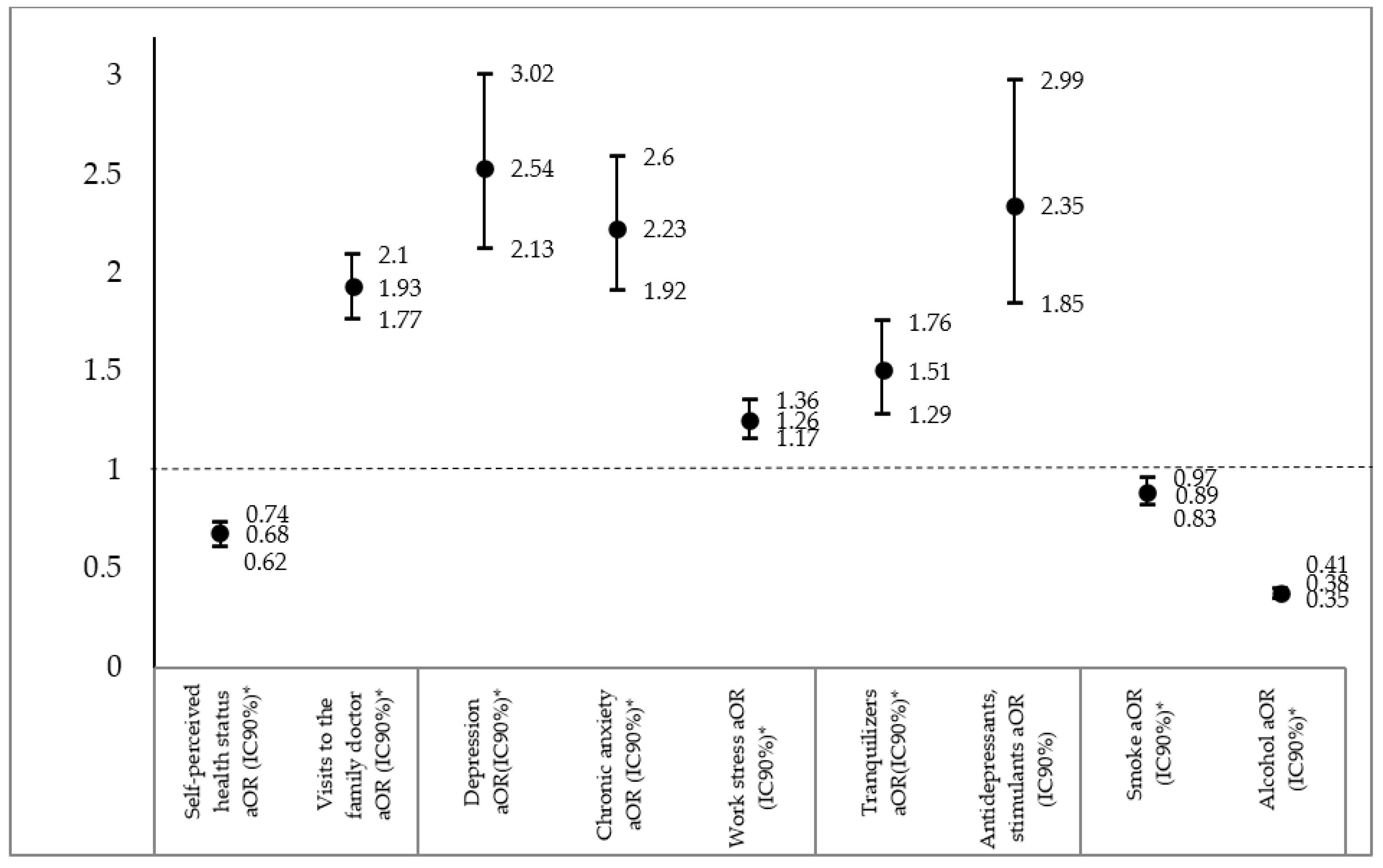
The regression models (Figure 1), would confirm the associations found in the descriptive analyses, to the extent that women were 1.47 times more likely to report poor health perceived by themselves than men (aOR = 0.68; IC90%:0.62–0.74) and 1.93 times more likely to visit the family doctor (aOR = 1.93; IC90%:1.77–2.1). In addition, women had a worse mental health status as they were 2.54 times more likely to suffer from depression (aOR = 2.54; IC90%:2.13–3.02), 2.23 and 1.26 times more likely to remit chronic anxiety and stress, respectively, compared to men. A similar situation occurred in the consumption of hypnosedatives, since women were more likely to consume tranquilizers (aOR = 1.51; IC90%:1.29–1.76) and antidepressants (aOR = 2.35; IC90%:1.85–2.99). However, men were 2.63 times more likely to consume alcohol (aOR = 0.38; IC90%: 0.35–0.41).

In order to deepen the analysis of the differences between the male and female labor force, regressions of the nine health and consumption indicators were carried out with the interactions between gender and the type of labor relationship and the occupational social class. The results obtained (Table 2) show that the gender differences found in Figure 1 increase both in work situations and in more vulnerable social classes. Specifically, women working without a contract were found to be 4.03 times more likely to suffer from depression (aOR = 4.03; IC90% = 2.22–7.3), 3.96 times more likely to report chronic anxiety (aOR = 3.96; IC90% = 2.2–7), or 4.01 times more likely to take antidepressants (aOR = 4.01; IC90% = 1.92–8.3) than men working without a contract. Similar situations were identified in unemployed women who were more likely to suffer from depression (aOR = 3.19; IC90% = 2.71–3.2), chronic anxiety (aOR = 3.15; IC90% = 2.69–3.6) and antidepressant use (aOR = 2.95; IC90% = 2.36–3.69) compared to unemployed men. With regard to the social occupational class, the most relevant gender differences were also found in psychosomatic pathologies and the consumption of hypnosedatives among both qualified and unqualified manual technicians, although these associations were less intense.

3.1. Relationships between Socio-Labour Characteristics and Consumption Indicators in the Male Labour Force

Regression analyses on the male labor force (Table 3) found how unemployment correlated with poorer health and consumption standards, as unemployed workers were 1.75 times more likely to report poorer self-perceived health (aOR = 0.57; IC90%: 0.38–0.89), 5.53 and 5.92 times more likely to suffer from depression and chronic anxiety, respectively (aOR = 5.53; IC90%:2.49–12.26; aOR = 5.92; IC90%: 2.83–12.42, respectively), compared to employers. In addition, unemployed workers were also more likely to use tranquilizers (aOR = 3.09; IC90%: 1.60–5.95), antidepressants (aOR = 6.75; IC90%: 1.91–23.83), and tobacco (aOR = 1.75; IC90%: 1.28–2.41). However, the employers presented greater probability of suffering labor stress with respect to the rest of labor situations, arriving to present 1.56 times larger probabilities of referring to stress than the workers without a contract (aOR = 0.64; IC90%: 0.51–0.79). In addition, employers were more likely to consume alcohol than unemployed workers (aOR = 0.51; IC90%: 0.37–0.71).

In reference to occupational social class, both skilled and unskilled manual technicians were associated with worse health standards (general and mint) and consumption of hypnosedatives compared to managers with more than 10 employees. Nevertheless, the highest differences were found in unskilled manual workers who were 1.75 times more likely to have worse self-perceived health status (aOR = 0.57; CI90%: 0.48–0.69), as well as being more likely to suffer from depression (aOR = 2.39; IC90%: 1.67–3.44), chronic anxiety (aOR = 2.40; IC90%: 1.71–3.42) and to take tranquilizers (aOR = 1.92; IC90%: 1.44–2.56), antidepressants (aOR = 2.30; IC90%: 1.42–3.71) or tobacco (aOR = 2.62; IC90%: 2.19–3.13). However, managers with more than 10 employees were 1.96 times more likely to report job stress (aOR = 0.51; IC90%: 0.40–0.63) and 1.47 more likely to consume alcohol (aOR = 0.68; IC90%: 0.58–0.80) compared to unskilled manual technicians.

Finally, the most noteworthy results regarding working time were that, on the one hand, part-time workers reported a smaller likelihood of suffering work stress (aOR = 0.60; IC90%: 0.49–0.7) and, on the other hand, that those who worked shifts appeared more likely to report a worse state of self-perceived health (aOR = 0.82; IC90%: 0.52–0.99), visiting their family doctor more (aOR = 1.25; IC90%: 1.07–1.40) and reporting chronic anxiety (aOR = 01.67; IC90%: 1.21–2.3) compared to those who worked split shifts.

3.2. Relationships between Socio-Labour Characteristics and Consumption Indicators in the Female Labour Force

In reference to the female labor force, the results obtained (Table 4) showed similar findings to those identified in men regarding the labor situation, insofar as unemployed women presented a lower probability of referring to a good state of self-perceived health (aOR = 0.56; IC90%: 0.39–0.79) and a higher probability of suffering from depression (aOR = 2.70; IC90%: 1.59–4.58), chronic anxiety (aOR = 2.00; IC90%: 1.23–3.26) or taking tranquilizers (aOR = 2.29; IC90%: 1.30–4.00) and tobacco (aOR = 1.92; IC90%: 1.03–3.61) with respect to female entrepreneurs. However, the highest probabilities were found in women working without a contract, who were 1.92 times more likely to suffer from depression (aOR = 1.92; IC90%: 1.12–4.1) and 2.60 times more likely to smoke tobacco (aOR = 2.60; IC90%: 1.01–6.70) than female entrepreneurs. Furthermore, coinciding again with the results for the male workforce, associations were observed between female managers and work stress or alcohol consumption, insofar as women working without a contract were less likely to suffer work stress (aOR = 0.62; IC90%: 0.36–0.8) or consume alcohol (aOR = 0.56; IC90%: 0.3–0.98) than female entrepreneurs.

In reference to occupational social class, again, coinciding with men, both qualified and unqualified manual techniques were associated with worse health and consumption of hypnosedatives compared to managers with more than 10 employees. The largest differences were found in unskilled manual workers who were 1.61 more likely to have worse self-perceived health (aOR = 0.62; CI90%: 0.53–0.72), as well as a higher probability of suffering from depression (aOR = 1.82; IC90%: 1.46–2.27) or chronic anxiety (aOR = 1.76; IC90%: 1.41–2.20) and of taking tranquilizers (aOR = 1.52; IC90%: 1.24–1.87), antidepressants (aOR = 1.69; IC90%: 1.28–2.23) or tobacco (aOR = 1.96; IC90%: 1.64–2.33). However, managers with more than 10 employees were 1.39 times more likely to report job stress (aOR = 0.72; IC90%: 0.58–0.89) and 2.00 times more likely to consume alcohol (aOR = 0.50; IC90%: 0.43–0.57) compared to unskilled manual technicians.

Finally, with reference to the working day, unlike the male working population, women working the afternoon shift or irregular days were those who presented the most significant associations with general and mental health indicators. Women working continuous afternoon shifts were 1.56 times more likely to report self-perceived ill health (aOR = 0.64; IC90%: 0.48–0.84), 2.38 times more likely to suffer from depression (aOR = 2.38; IC90%:1.63–3.4) and 1.95 times more likely to suffer from chronic anxiety (aOR = 1.95; IC90%: 1.35–2.8) than women working split shifts. On the other hand, workers with irregular working hours also presented a higher likelihood of reporting depression (aOR = 1.56; IC90%: 1.14–2.1), chronic anxiety (aOR = 1.35; IC90%: 1.01–1.8) and consumption of tranquilizers (aOR = 1.59; IC90%: 1.16–2.1). In terms of working time, part-time workers were more likely to suffer from depression (aOR = 1.50; IC90%: 1.22–1.8) and less likely to report job-related stress (aOR = 0.59; IC90%: 0.40–0.61).

4. Discussion

The results obtained (Table 1 and Figure 1) confirm some results of previous studies, as the prevalence of poor self-perceived health, mental disorders and hypnosedative use is higher in women [77,78], while alcohol consumption is higher in men [77,78,79]. Furthermore, as shown in Table 2, the differences between men and women increase in the most unstable employment situations (working without a contract or unemployed) and in the most vulnerable occupational social classes (skilled and unskilled manual workers) to the extent that the odds ratios identified in these categories are higher both in psychosomatic pathologies and in the consumption of hypnosedatives.

Likewise, it is confirmed for both sexes that unemployment is related to worse self-perceived health, the fact of suffering from depression and the consumption of hypnosedatives [51,54,77]. However, as noted in the introduction, subjective employability could influence as a possible moderator the relationship between job insecurity and negative mental health outcomes. It would be interesting in future studies to have measurement variables of subjective employability to observe their interaction with attributed job insecurity and health and consumption outcomes.

Continuing with the analysis, it is worth mentioning that the impact of unemployment is greater among the male labor force for several reasons. First, because unemployed workers are more than twice as likely to suffer from depression as employed women. Second, while the unemployed have had a high prevalence of chronic anxiety and antidepressant use compared to actively working men, no differences in antidepressant use have been found between currently working and unemployed women, and the relationships identified for chronic anxiety are much smaller than those of men. This situation could be explained by the division of family roles and responsibilities between men and women, as previous studies have shown [60,80]. However, these hypotheses merit specific analysis in future studies, rather than the multidimensional analysis sought in this research, since, while there are important differences between the probabilities of the female and male workforces, when the sample is stratified by sex, they are no longer comparable.

Previous research has found that temporary workers and those with job instability make less frequent visits to the family doctor [55] and have a higher prevalence of mental disorders [53]. However, in our study we found that self-employed workers are the least likely to make medical visits and the most likely to suffer from depression and chronic anxiety. Despite the divergences between the results and the complexity of the relationships, there may be a pattern derived from the stronger perception of distress among precarious workers when they perceive high job insecurity [53], which may lead them not to absent themselves from work for fear of being fired and, consequently, not attending the doctor and opting to self-medicate. In fact, the Sixth European Survey on Working Conditions 2015 [81], identified that 44% of workers with permanent contracts declared that they had worked while sick during the last year, while among self-employed workers the rate was 50%, which could confirm that the productive need makes the self-employed worker not absent from work, even if he is sick. On the other hand, a study conducted in public hospitals identified that professionals with temporary employment contracts were more likely to self-medicate [82], which would explain why people who feel a high degree of job insecurity, whether as self-employed or temporary workers, tend not to be absent from work when they have health problems, and opt for self-medication. However, these hypotheses should be evaluated in future research. We could also consider that the precarious working conditions to which temporary workers are subjected may mean that they do not have sufficient financial resources to take out private health insurance and therefore go to the doctor less often. However, Spain has a universal health system, so this hypothesis for the Spanish case would be ruled out.

Since the aim of this research is to explore and describe, as a whole, the associations between factors of job insecurity and the different health and consumption indicators, we can observe different relationship patterns, depending on the work situation and the occupational social class. On the one hand, it has been identified that unemployed people, who belong to the most vulnerable social classes, suffer more frequently depression and chronic anxiety. These mental disorders, in turn, are associated, as shown by previous studies, with the increased consumption of hypnosedatives [58] and tobacco [83]. This would explain, to a certain extent, the patterns and associations of social vulnerability with mental disorders, consumption of hypnosedatives and tobacco obtained in our study.

The occupational classes with the highest status in Table 3 and Table 4, on the other hand, have reported greater stress than manual occupational classes, and both male and female managers with more than 10 employed people have also reported greater job stress, which would refute the findings identified in previous studies [84]. The greater occupational stress of these groups could be derived from the intensification of work in the most qualified “knowledge” jobs as they are more intensely exposed than manual workers to psychosocial risk factors such as emergencies to perform tasks, time pressure, speed or short term in the execution of work, role dysfunction, self-management, etc. [85,86,87,88,89,90]. The fact that the occupational classes with the highest status are also associated with the highest alcohol consumption would in turn confirm other previous findings [54]. There are two hypotheses that could explain the higher alcohol consumption in the better-positioned occupational social classes. The first is that differences in consumption across classes are explained by cultural patterns and by reduced access to such substances by blue-collar workers [54]. The second hypothesis is that higher consumption of alcohol by these groups is associated with a greater need to combat stress [57]. Both hypotheses could explain the relationships found in this study between occupational social classes with higher status, work stress and alcohol consumption.

We can also see the influence of the relationship between professional situation and social class on working time. On the one hand, if we consider (albeit with certain nuances) that part-time work is part of precarious employment [74], the results obtained show that this partiality is associated with a higher prevalence of depression in women. On the other hand, the results show that full-time work is associated with greater job stress in both sexes. Previous studies record similar results, insofar as this research has associated a higher number of working hours with higher occupational stress [55].

Finally, with regard to the type of working day, the results obtained show significant differences between the sexes. Although few associations have been identified in men, with shift work being the most damaging to general and mental health, multiple associations have been identified in women. In particular, it should be noted that the continuous afternoon shift is the one with the highest prevalence of depression and chronic anxiety, while the irregular shift is also associated with the highest probability of suffering from depression, chronic anxiety and the use of tranquilizers. These results differ from those of previous studies associating mental disorders with shift work [56,91], and further research is needed to improve the understanding of this relationship. However, it was observed that while the work situation or occupational social class affected men more, the type of working day affected women more. This could again be explained by the division of gender roles, which implies a greater workload for women in the family setting [60,80].

Limitations

The study presents some common limitations of the use of this type of survey. Firstly, the most important limitation is that there may be a risk of reverse causality, and therefore the findings identified should be considered as associations rather than causal relationships. This is a common limitation in this type of study [56,57,58,59,60,61]. Secondly, except for Figure 1 and Table 2, in which differences between men and women can be compared, the results obtained from the separate regressions for the male and female labor force (Table 3 and Table 4), as explained in the discussion, do not have comparable parameters, since the variance-covariance matrix is calculated separately. This situation would also occur in work of a similar nature [56,57,58,59,60,61]. However, it should be remembered that the objective of the research is to look for patterns that will allow more concrete comparative analyses to be carried out in future studies. Thirdly, there could be information and response biases of complacency on the part of participants, or of responding to what is considered socially acceptable. In this sense, more favored social classes and men, associated with stronger and more powerful roles, may be unwilling to acknowledge certain health problems because of social stigma. This attitude may result in an underrecording of mental pathologies or substance use. In fact, this situation could explain the low number of affirmative responses about mental disorders (depression or chronic anxiety) or the high number of unanswered cases about the use of hypnosedatives. On the other hand, there could be selection bias, for example, in the most vulnerable occupational classes due to the possibility of dropouts, or the increase in the number of unanswered questions. All this may favor the underregistration of pathologies and consumption. In addition, the underrepresentation of some categories (e.g., non-contract work, shift work, night work) prevents some more comprehensive stratified analyses. In the future it might be interesting to stratify the analysis by sex and age simultaneously or by a more disaggregated occupational social class, but the sample size would only allow a subset of analysis in those cases, leading to a reduction of possible analyses. The impossibility of having socio-occupational variables (e.g., number of working hours, production rates, social support) can also act as a confounder. It would therefore be useful to include them in future editions of the ENSE survey. Finally, it is worth mentioning that the associations found cannot be evaluated as “causal”, since this is a transversal study.

5. Conclusions

In conclusion, we believe that the study is relevant, since the exploration of health and consumption patterns can serve as a reference for the planning of sustainable preventive occupational health policies, both in labor and health institutions and in companies. These programs should focus, at least, on the unemployed, those who belong to the most vulnerable occupational social classes and considering the gender differences described. Specifically, two patterns of health erosion have been identified as a result of high rates of job insecurity. On the one hand, the most vulnerable people (unemployed and manual workers) suffer with a higher prevalence of depression, chronic anxiety, hypnosedative use and tobacco consumption, and therefore active employment policies should be promoted to reduce the high unemployment rates that still exist in Spain. On the other hand, more qualified people and, above all, managers have reported greater work stress and alcohol consumption. The problem of these groups does not lie so much in sustaining employment, but rather in the deregulation of working conditions which has led to an increase in the intensification of employment, which is a determining factor in the increase of work-related stress and alcohol consumption. To all this, we should add another series of policies to reconcile work and family life (for example, reducing working hours and establishing schedules compatible with reproductive tasks), since, as we have seen, it affects working women in particular in a negative way. It seems reasonable, therefore, to call for the revival of social dialogue for the implementation of sustainable measures to improve the quantity and quality of employment, since neoliberal policies for the management of the economic crisis have caused a serious public health problem. However, it should be remembered that this study is of an exploratory nature, and therefore, rather than directly suggesting courses of action, it highlights the need to increase research into labor relations and occupational health, and then, on that basis, to implement specific labor and health policies.

References

- Rigby, M.; García-Calavia, M.Á. Institutional resources as a source of trade union power in Southern Europe. Eur. J. Ind. Relat. 2018, 24, 129–143. [Google Scholar] [CrossRef]
- Barranco, O.; Molina, Ó. Sindicalismo y crisis económica: Amenazas, retos y oportunidades. Kultur Rev. Interdisc. Sobre Cult. Ciutat 2014, 1, 171–194. [Google Scholar] [CrossRef] [Green Version]
- Benner, M. Before and Beyond the Global Economic Crisis; Edward Elgar: Cheltenham, UK, 2013. [Google Scholar]
- Gago, A. Crisis, cambio en la UE y estrategias sindicales: El impacto de la condicionalidad en el repertorio estratégico de los sindicatos españoles durante la crisis de la eurozona. Rev. Esp. Cienc. Polít. 2016, 42, 45–68. [Google Scholar] [CrossRef] [Green Version]
- Beneyto, P.J.; Alós, R.; Jódar, P.; Vidal, S. La afiliación sindical en la crisis Estructura, evolución y trayectorias. Sociol. Trab. 2016, 87, 25–44. [Google Scholar]
- Lehndorff, S. Acting in different worlds. Challenges to transnational trade union cooperation in the eurozone crisis. Transf. Eur. Rev. Labour Res. 2015, 21, 157–170. [Google Scholar] [CrossRef]
- Stuckler, D.; Basu, S.; Suhrcke, M.; Coutts, A.; McKee, M. The public health effect of economic crises and alternative policy responses in Europe: An empirical analysis. Lancet 2009, 374, 315–323. [Google Scholar] [CrossRef]
- Stuckler, D.; King, L.; McKee, M. Mass Privatisation and the Post-Communist Mortality Crisis: A Cross-National Analysis. Lancet 2009, 373, 399–407. [Google Scholar] [CrossRef]
- Bacigalupe, A.; Martín, U.; Font, R.; González-Rábago, Y.; Bergantiños, N. Austeridad y privatización sanitaria en época de crisis: ¿existen diferencias entre las comunidades autónomas? Gac. Sanit. 2016, 30, 47–51. [Google Scholar] [CrossRef] [Green Version]
- Cabrera-León, A.; Codina, A.D.; Mateo, I.; Arroyo-Borrell, E.; Bartoll, X.; Bravo, M.J.; Domínguez-Berjón, M.F.; Renart, G.; Álvarez-Dardet, C.; Marí-Dell’Olmo, M.; et al. Indicadores contextuales para evaluar los determinantes sociales de la salud y la crisis económica española. Gac. Sanit. 2017, 31, 194–203. [Google Scholar] [CrossRef] [Green Version]
- Del Pozo-Rubio, R.; Pardo-García, I.; Escribano-Sotos, F. El copago de dependencia en España a partir de la reforma estructural de 2012. Gac. Sanit. 2017, 31, 23–29. [Google Scholar] [CrossRef] [Green Version]
- Ferrando, J.; Palència, L.; Gotsens, M.; Puig-Barrachina, V.; Marí-Dell’Olmo, M.; Rodríguez-Sanz, M.; Bartoll, X.; Borrell, C. Trends in cancer mortality in Spain: The influence of the financial crisis. Gac. Sanit. 2019, 33, 229–234. [Google Scholar] [CrossRef] [PubMed]
- Porthé, V.; Vargas, I.; Ronda, E.; Malmusi, D.; Bosch, L.; Vázquez, M.L. Has the quality of health care for the immigrant population changed during the economic crisis in Catalonia (Spain)? Opinions of health professionals and immigrant users. Gac. Sanit. 2018, 32, 425–432. [Google Scholar] [CrossRef] [PubMed]
- Benavides, F.G.; Delclós, J.; Serra, C. Estado de bienestar y salud pública: El papel de la salud laboral. Gac. Sanit. 2018, 32, 377–380. [Google Scholar] [CrossRef]
- Sverke, M.; Hellgren, J.; Näswall, K. No Security: A Meta-Analysis and Review of Job Insecurity and Its Consequences. J. Occup. Health Psychol. 2002, 7, 242–264. [Google Scholar] [CrossRef] [PubMed]
- Valenzuela, H.C. Precariedad, precarización y trabajo precario. Polis 2015, 40, 313–329. [Google Scholar]
- Shoss, M.K. Job insecurity: An integrative review and agenda for future research. J. Manag. 2017, 43, 1911–1939. [Google Scholar] [CrossRef]
- Green, F. Demanding Work: The Paradox of Job Quality in the Affluent Economy; Princeton University Press: Oxford, UK, 2006. [Google Scholar]
- Büssing, A. Can Control at Work and Social Support Moderate Psychological Consequences of Job Insecurity? Results from a Quasi-experimental Study in the Steel Industry. Eur. J. Work. Organ. Psychol. 1999, 8, 219–242. [Google Scholar] [CrossRef]
- Green, F. Unpacking the misery multiplier: How employability modifies the impacts of unemployment and job insecurity on life satisfaction and mental health. J. Health Econ. 2011, 30, 265–276. [Google Scholar] [CrossRef] [Green Version]
- Green, F.; Mostafa, T. Trends in Job Quality in Europe; Publications Office of the European Union: Luxembourg, 2012. [Google Scholar]
- Greenhalgh, L.; Rosenblatt, Z. Job Insecurity: Toward Conceptual Clarity. Acad. Manag. Rev. 1984, 9, 438. [Google Scholar] [CrossRef] [Green Version]
- Stock, R. Socio-Economic Security, Justice and the Psychology of Social Relationships; International Labour Office: Geneva, Switzerland, 2001. [Google Scholar]
- Klandermans, B.; Hesselink, J.K.; van Vuuren, T. Employment status and job insecurity: On the subjective appraisal of an objective status. Econ. Ind. Democr. 2010, 31, 557–577. [Google Scholar] [CrossRef]
- De Witte, H.; Näswall, K. “Objective” vs “Subjective” Job Insecurity: Consequences of Temporary Work for Job Satisfaction and Organizational Commitment in Four European Countries. Econ. Ind. Democr. 2003, 24, 149–188. [Google Scholar] [CrossRef]
- Benach, J.; Vives, A.; Amable, M.; Vanroelen, C.; Tarafa, G.; Muntaner, C. Precarious Employment: Understanding an Emerging Social Determinant of Health. Annu. Rev. Public Health 2014, 35, 229–253. [Google Scholar] [CrossRef] [PubMed] [Green Version]
- Ferrie, J.E.; Westerlund, H.; Virtanen, M.; Vahtera, J.; Kivimäki, M. Flexible labor markets and employee health. SJWEH 2008, 6, 98–110. [Google Scholar]
- Dickerson, A.; Green, F. Fears and realisations of employment insecurity. Labour Econ. 2012, 19, 198–210. [Google Scholar] [CrossRef] [Green Version]
- Chung, H. Dualization and subjective employment insecurity: Explaining the subjective employment insecurity divide between permanent and temporary workers across 23 European countries. Econ. Ind. Democr. 2016, 40, 700–729. [Google Scholar] [CrossRef] [Green Version]
- De Cuyper, N.; De Witte, H. Temporary Employment and Perceived Employability: Mediation by Impression Management. J. Career Dev. 2010, 37, 635–652. [Google Scholar] [CrossRef]
- Heponiemi, T.; Elovainio, M.; Pentti, J.; Virtanen, M.; Westerlund, H.; Virtanen, P.; Oksanen, T.; Kivimäki, M.; Vahtera, J. Association of Contractual and Subjective Job Insecurity with Sickness Presenteeism Among Public Sector Employees. J. Occup. Environ. Med. 2010, 52, 830–835. [Google Scholar] [CrossRef]
- Virtanen, M.; Kivimäki, M.; Elovainio, M.; Vahtera, J.; Ferrie, J. From insecure to secure employment: Changes in work, health, health related behaviours, and sickness absence. Occup. Environ. Med. 2003, 60, 948–953. [Google Scholar] [CrossRef]
- López-Gómez, M.A.; Durán, X.; Zaballa, E.; Sanchez-Niubo, A.; Delclos, G.L.; Benavides, F.G. Cohort profile: The Spanish WORKing life Social Security (WORKss) cohort study. BMJ Open 2016, 6, e8555. [Google Scholar] [CrossRef] [Green Version]
- Serra, L.; López-Gómez, M.A.; Sanchez-Niubo, A.; Delclos, G.L.; Benavides, F.G. Application of latent growth modeling to identify different working life trajectories: The case of the Spanish WORKss cohort. Scand. J. Work. Environ. Health 2016, 43, 42–49. [Google Scholar] [CrossRef]
- Kivimäki, M.; Vahtera, J.; Pentti, J.; Ferrie, J. Factors underlying the effect of organisational downsizing on health of employees: Longitudinal cohort study. BMJ 2000, 320, 971–975. [Google Scholar] [CrossRef] [PubMed] [Green Version]
- Vahtera, J.; Kivimäki, M.; Pentti, J.; Linna, A.; Virtanen, M.; Virtanen, P.; Ferrie, J. Organisational downsizing, sickness absence, and mortality: 10-town prospective cohort study. BMJ Clin. Res. Ed. 2004, 328, 555. [Google Scholar] [CrossRef] [Green Version]
- Marler, J.H.; Woodard-Barringer, M.; Milkovich, G.T. Boundaryless and traditional contingent employees: Worlds apart. J. Organ. Behav. 2002, 23, 425–453. [Google Scholar] [CrossRef]
- Cano, E. La extensión de la precariedad laboral como norma social. Soc. Y Utopía Rev. De Cienc. Soc. 2007, 29, 117–138. [Google Scholar]
- Katz, L.F.; Krueger, A.B. The Rise and Nature of Alternative Work Arrangements in the United States, 1995–2015. ILR Rev. 2018, 72, 382–416. [Google Scholar] [CrossRef] [Green Version]
- Aronsson, G.; Gustafsson, K.; Dallner, M. Work environment and health in different types of temporary jobs. Eur. J. Work. Organ. Psychol. 2002, 11, 151–175. [Google Scholar] [CrossRef]
- Fiori, F.; Rinesi, F.; Spizzichino, D.; Di Giorgio, G. Employment insecurity and mental health during the economic recession: An analysis of the young adult labour force in Italy. Soc. Sci. Med. 2016, 153, 90–98. [Google Scholar] [CrossRef] [Green Version]
- Hammarström, A. Health consequences of youth unemployment—Review from a gender perspective. Soc. Sci. Med. 1994, 38, 699–709. [Google Scholar] [CrossRef]
- Granado, A.E. Crisis económica, políticas, desempleo y salud (mental). Rev. Asoc. Española Neuropsiquiatría 2014, 34, 385–404. [Google Scholar] [CrossRef] [Green Version]
- Serrano-Rosa, M.A.; Baena, S.; Molins-Correa, F. Diferencias entre empleabilidad, inseguridad laboral y salud en trabajadores y desempleados. Acción Psicológica 2018, 15, 87–102. [Google Scholar] [CrossRef] [Green Version]
- Berntson, E.; Marklund, S. The Relationship Between Perceived Employability and Subsequent Health. Work Stress 2007, 21, 279–292. [Google Scholar] [CrossRef]
- Vanhercke, D.; De Cuyper, N.; Peeters, E.; De Witte, H. Defining Perceived Employability: A Psychological Approach. Pers. Rev. 2014, 43, 592–605. [Google Scholar] [CrossRef]
- de Grip, A.; van Loo, J.; Sanders, J. The Industry Employability Index: Taking Account of Supply and Demand Characteristics. Int. Labour Rev. 2004, 143, 211–233. [Google Scholar] [CrossRef] [Green Version]
- Allebeck, P. Health Effects of the Crisis: Challenges for Science and Policy. Eur. J. Public Health 2013, 23, 721. [Google Scholar] [CrossRef] [PubMed] [Green Version]
- Bernal, J.L.; Gasparrini, A.; Artundo, C.M.; McKee, M. The Effect of the Late 2000s Financial Crisis on Suicides in Spain: An Interrupted Time-Series Analysis. Eur. J. Public Health 2013, 23, 732–736. [Google Scholar] [CrossRef] [Green Version]
- Salvador-Carulla, L.; Roca, M. Mental Health Impact of the Economic Crisis in Spain. Int. J. Psychiatry 2013, 10, 8–10. [Google Scholar]
- Urbanos-Garrido, R.; López-Valcárcel, B.G. The influence of the economic crisis on the association between unemployment and health: An empirical analysis for Spain. Eur. J. Health Econ. 2014, 16, 175–184. [Google Scholar] [CrossRef]
- Bartoll, X.; Palència, L.; Malmusi, D.; Suhrcke, M.; Borrell, C. The evolution of mental health in Spain during the economic crisis. Eur. J. Public Health 2013, 24, 415–418. [Google Scholar] [CrossRef] [Green Version]
- Sirviö, A.; Ek, E.; Jokelainen, J.; Koiranen, M.; Järvikoski, T.; Taanila, A. Precariousness and discontinuous work history in association with health. Scand. J. Public Health 2012, 40, 360–367. [Google Scholar] [CrossRef]
- Benavides, F.G.; Ruiz-Forès, N.; Delclós, G.; Domingo-Salvany, A. Consumo de alcohol y otras drogas en el medio laboral en España. Gac. Sanit. 2013, 27, 248–253. [Google Scholar] [CrossRef] [Green Version]
- Arias-Uriona, A.M.; Ordóñez, J.C. Factores de precariedad laboral y su relación con la salud de trabajadores en Bolivia. Rev. Panam. Salud Pública 2018, 42, e98. [Google Scholar] [CrossRef] [PubMed]
- García-Díaz, V.; Fernández-Feito, A.; Arias, L.; Lana, A. Consumo de tabaco y alcohol según la jornada laboral en España. Gac. Sanit. 2015, 29, 364–369. [Google Scholar] [CrossRef] [PubMed] [Green Version]
- Colell, E.; Sanchez-Niubo, A.; Benavides, F.G.; Delclos, G.L.; Domingo-Salvany, A. Work-related stress factors associated with problem drinking: A study of the Spanish working population. Am. J. Ind. Med. 2014, 57, 837–846. [Google Scholar] [CrossRef] [PubMed] [Green Version]
- Colell, E.; Sanchez-Niubo, A.; Ferrer, M.; Domingo-Salvany, A. Gender differences in the use of alcohol and prescription drugs in relation to job insecurity. Testing a model of mediating factors. Int. J. Drug Policy 2016, 37, 21–30. [Google Scholar] [CrossRef] [PubMed] [Green Version]
- Colell, E.; Sánchez-Niubò, A.; Domingo-Salvany, A.; Delclos, G.; Benavides, F.G. Prevalencia de consumo de hipnosedantes en población ocupada y factores de estrés laboral asociados. Gac. Sanit. 2014, 28, 369–375. [Google Scholar] [CrossRef] [Green Version]
- Arias de la Torre, J.; Molina, A.J.; Fernández-Villa, T.; Artazcoz, L.; Martín, V. Mental health, family roles and employment status inside and outside the household in Spain. Gac. Sanit. 2019, 33, 235–241. [Google Scholar] [CrossRef]
- Virtanen, M.; Honkonen, T.; Kivimäki, M.; Ahola, K.; Vahtera, J.; Aromaa, A.; Lönnqvist, J. Work stress, mental health and antidepressant medication findings from the Health 2000 Study. J. Affect. Disord. 2007, 98, 189–197. [Google Scholar] [CrossRef]
- Wang, J. Work stress as a risk factor for major depressive episode(s). Psychol. Med. 2004, 35, 865–871. [Google Scholar] [CrossRef]
- Romelsjö, A.; Stenbacka, M.; Lundberg, M.; Upmark, M. A population study of the association between hospitalization for alcoholism among employees in different socio-economic classes and the risk of mobility out of, or within, the workforce. Eur. J. Public Health 2004, 14, 53–57. [Google Scholar] [CrossRef] [Green Version]
- Artazcoz, L.; Cortès, I.; Borrell, C.; Escribà-Agüir, V.; Cascant, L. Social inequalities in the association between partner/marital status and health among workers in Spain. Soc. Sci. Med. 2011, 72, 600–607. [Google Scholar] [CrossRef]
- Arcas, M.M.; Novoa, A.M.; Artazcoz, L. Gender inequalities in the association between demands of family and domestic life and health in Spanish workers. Eur. J. Public Health 2012, 23, 883–888. [Google Scholar] [CrossRef] [PubMed] [Green Version]
- Krieger, N. Genders, sexes, and health: what are the connections—And why does it matter? Int. J. Epidemiol. 2003, 32, 652–657. [Google Scholar] [CrossRef] [PubMed]
- Messing, K.; Mager Stellman, J. Sex, gender and women’s occupational health: The importance of considering mechanism. Environ. Res. 2006, 101, 149–162. [Google Scholar] [CrossRef]
- Hankivsky, O.; Christoffersen, A. Intersectionality and the determinants of health: A Canadian perspective. Crit. Public Health 2008, 18, 271–283. [Google Scholar] [CrossRef]
- Hankivsky, O. Women’s health, men’s health, and gender and health: Implications of intersectionality. Soc. Sci. Med. 2012, 74, 1712–1720. [Google Scholar] [CrossRef]
- Ministerio De Sanidad Consumo Y Bienestar Social. Encuesta Nacional de Salud 2017. ENSE 2017 Metodología. 2017. Available online: https://www.ine.es/metodologia/t15/t153041917.pdf11 (accessed on 24 March 2020).
- Henares-Montiel, J.; Ruiz-Pérez, I.; Sordo, L. Salud mental en España y diferencias por sexo y por comunidades autónomas. Gac. Sanit. 2020, 34, 114–119. [Google Scholar] [CrossRef]
- Beneyto, P.J.; Payá, R. Mercado de trabajo y estructura ocupacional. In Estructura Social Contemporánea; Perelló, S., Ed.; Tirant lo Blanch: Valencia, Spain, 2019; pp. 169–204. [Google Scholar]
- Croezen, S.; Burdorf, A.; Van Lenthe, F.J. Self-perceived health in older Europeans: Does the choice of survey matter? Eur. J. Public Health 2016, 26, 686–692. [Google Scholar] [CrossRef] [Green Version]
- Gumà, J.; Arpino, B.; Solé-Auró, A. Determinantes sociales de la salud de distintos niveles por género: Educación y hogar en España. Gac. Sanit. 2019, 33, 127–133. [Google Scholar] [CrossRef]
- De Bruin, A.; Picavet, H.S.J.; Nossikov, A. Health Interview Surveys. Towards Interna-Tional Harmonization of Methods and Instruments; WHO Regional Office for Europe: Copenhagen, Denmark, 1996. [Google Scholar]
- Simó-Noguera, C.; Hernández-Monleón, A.; Muñoz-Rodríguez, D.; González-Sanjuán, M.E. El efecto del estado civil y de la convivencia en pareja en la salud. Rev. Española Investig. Sociológicas 2015, 151, 141–166. [Google Scholar] [CrossRef]
- Teixidó-Compañó, E.; Espelt, A.; Sordo, L.; Bravo, M.J.; Sarasa-Renedo, A.; Indave, B.I.; Bosque-Prous, M.; Brugal, M.T. Differences between men and women in substance use: The role of educational level and employment status. Gac. Sanit. 2018, 32, 41–47. [Google Scholar] [CrossRef]
- Wittchen, H.U.; Jacobi, F.; Rehm, J.; Gustavsson, A.; Svensson, M.; Jönsson, B.; Olesen, J.; Allgulander, C.; Alonso, J.; Faravelli, C.; et al. The size and burden of mental disorders and other disorders of the brain in Europe 2010. Eur. Neuropsychopharmacol. 2011, 21, 655–679. [Google Scholar] [CrossRef] [PubMed] [Green Version]
- Bosque-Prous, M.; Espelt, A.; Borrell, C.; Bartroli, M.; Guitart, A.M.; Villalbi, J.R.; Brugal, T. Gender differences in hazardous drinking among middle-aged in Europe: The role of social context and women’s empowerment. Eur. J. Public Health 2015, 25, 698–705. [Google Scholar] [CrossRef] [PubMed] [Green Version]
- Mäkelä, P.; Gmel, G.; Grittner, U.; Kuendig, H.; Kuntsche, S.; Bloomfield, K.; Room, R. Drinking patterns and their gender differences in Europe. Alcohol Alcohol. Suppl. 2006, 41, i8–i18. [Google Scholar] [CrossRef] [PubMed]
- Eurofound. European Working Conditions Survey 2015. Available online: https://www.eurofound.europa.eu/data/european-working-conditions-survey (accessed on 1 April 2020).
- Barros, A.R.R.; Griep, R.H.; Rotenberg, L. Self-medication among nursing workers from public hospitals. Rev. Latinoam. Enferm. 2010, 17, 1015–1022. [Google Scholar] [CrossRef]
- Sobradiel, N.; García-Vicent, V. Consumo de tabaco y patología psiquiátrica. Trastor. Adict. 2007, 9, 31–38. [Google Scholar] [CrossRef]
- Benavides, F.G.; Benach, J.; Román, C. Tipos de empleo y salud: Análisis de la segunda Encuesta Europea de Condiciones de Trabajo. Gac. Sanit. 1999, 13, 425–430. [Google Scholar] [CrossRef] [Green Version]
- Castillo, J.J.Y.; Agulló, I. Trabajo y Vida en la Sociedad de la Información. Un Distrito Tecnológico en el Norte de Madrid; La Catarata: Madrid, Spain, 2012. [Google Scholar]
- Sánchez, A.L. La participación de los trabajadores en la calidad total: Nuevos dispositivos disciplinarios de organización del trabajo. Rev. Española Investig. Sociológicas 2004, 106, 63. [Google Scholar] [CrossRef]
- Pérez-Zapata, O.; Alvarez-Hernández, G.; Castaño-Collado, C.; Lahera-Sánchez, A. Sostenibilidad y calidad del trabajo en riesgo: La intensificación del trabajo del conocimiento. Rev. Minist. Empl. Y Segur. Soc. 2015, 116, 175–214. [Google Scholar]
- Pinilla, J. La intensificación del esfuerzo de trabajo en España. Cuad. Relac. Labor. 2004, 22, 117–135. [Google Scholar]
- García, F.J.P.; López-Peláez, A. La intensificación del trabajo en España (2007–2011): Trabajo en equipo y flexibilidad. Rev. Española Investig. Sociológicas 2017, 160, 79–94. [Google Scholar] [CrossRef]
- Schieman, S.; Whitestone, Y.K.; van Gundy, K. The Nature of Work and the Stress of Higher Status. J. Health Soc. Behav. 2006, 47, 242–257. [Google Scholar] [CrossRef] [PubMed]
- Bøggild, H.; Knutsson, A. Shift work, risk factors and cardiovascular disease. Scand. J. Work. Environ. Health 1999, 25, 85–99. [Google Scholar] [CrossRef] [PubMed]
Figure 1.
Logistic regressions between health and consumption indicators by sex. OR: adjusted odds ratio for the four socio-labor variables included in the table (type of contract or employment situation, occupational category, household income, working time and type of working day) and the demographic variables (age, nationality, marital status, level of education, type of family life, family care work, monthly household income) with men as the reference category; IC90%: confidence interval; * significance level of the p-value < 0.10.