90 Days of COVID-19 Social Distancing and Its Impacts on Air Quality and Health in Sao Paulo, Brazil


Instituto de Ciências Ambientais, Químicas e Farmacêuticas, Universidade Federal de São Paulo (UNIFESP), Diadema 09913-030, Brazil
*
Author to whom correspondence should be addressed.
Sustainability 2020, 12(18), 7440; https://0-doi-org.brum.beds.ac.uk/10.3390/su12187440
Submission received: 8 August 2020
/
Revised: 4 September 2020
/
Accepted: 8 September 2020
/
Published: 10 September 2020
(This article belongs to the Special Issue Assessment of Socio-Economic Sustainability and Resilience after COVID-19)
Abstract
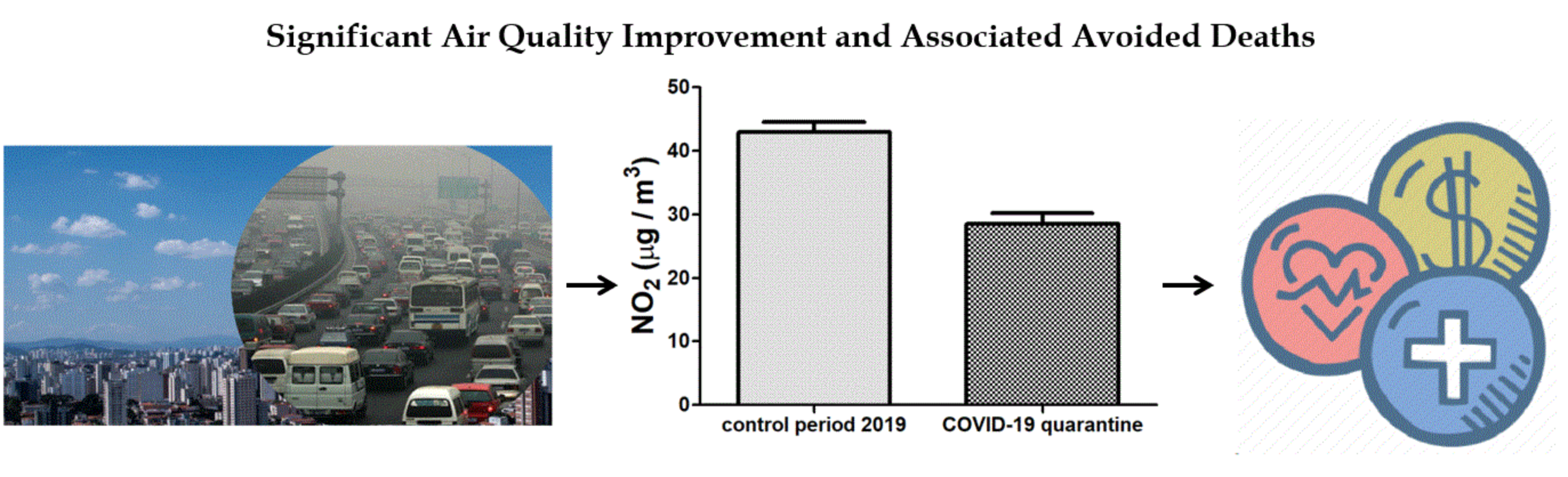
:The COVID-19 pandemic has imposed a unique situation for humanity, reaching up to 5623 deaths in Sao Paulo city during the analyzed period of this study. Due to the measures for social distancing, an improvement of air quality was observed worldwide. In view of this scenario, we investigated the air quality improvement related to PM10, PM2.5, and NO2 concentrations during 90 days of quarantine compared to an equivalent period in 2019. We found a significant drop in air pollution of 45% of PM10, 46% of PM2.5, and 58% of NO2, and using a relative-risk function, we estimated that this significant air quality improvement avoided, respectively, 78, 337, and 387 premature deaths, respectively, and prevented approximately US $720 million on health costs. Moreover, we estimated that 5623 deaths by COVID-19 represent an economic health loss of US $10.5 billion. Both health and economic gains associated with air pollution reductions give a positive perspective of the efforts towards keeping air pollution reduced even after the pandemic, highlighting the importance of improving the strategies of air pollution mitigation actions, as well as the crucial role of adopting efficient measures to protect human health both during and after the COVID-19 global health crisis.

1. Introduction
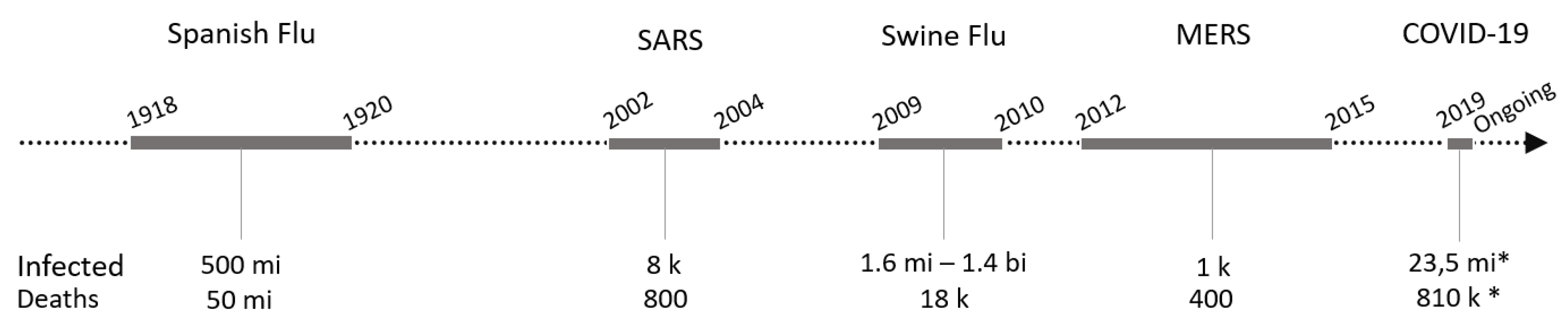
The coronavirus disease (COVID-19) pandemic caused by rapidly spreading a severe acute respiratory syndrome coronavirus 2 (SARS-CoV-2) has imposed a unique situation for humanity since the Spanish flu pandemic, transmitted by the H1N1 influenza A virus, which devastated at least 50 million people in 1918. Thus far, COVID-19 is considered the deadliest pandemic in modern history, exceeding the outbreaks caused by H1N1 virus, such as the most recent outbreak in 2009, formerly known as swine flu [1,2,3,4,5,6,7,8].
Likewise, in the past two decades, coronaviruses have also shown a continuing potential threat to public health since the emergence of severe acute respiratory syndrome coronavirus (SARS-CoV) and Middle East respiratory syndrome coronavirus (MERS-CoV). SARS-CoV and MERS-CoV can cause severe respiratory distress syndrome in humans, and despite SARS-CoV-2 being highly pathogenic and deadlier to humans, SARS epidemics (2003–2004) and MERS outbreaks (2012) were responsible for the deaths of thousands of people worldwide, as shown in Figure 1 [1,2,3,4,5,6,7,8].
Since its emergence in Wuhan, the capital of Hubei Province at the end of 2019, SARS-CoV-2 has quickly spread worldwide, characterizing a pandemic. On 30 January 2020, the Emergency Committee of the World Health Organization (WHO) declared a global health emergency based on the increasing rates of case reporting on different continents [10].
The first case in Latin America was confirmed in February 2020 in Sao Paulo city, Brazil. The confirmed patient had travelled to Lombardy in northern Italy, and the same origin was confirmed for the virus by genome sequencing [11]. Since then, an exponential increase in confirmed cases was observed in the following weeks. No specific drugs or vaccines are available, and health systems are overburdened in every city, especially in Sao Paulo city, which reported 91,198 confirmed cases of COVID-19 and 5623 deaths up to 14 June (last day of the analyzed period in this study), being considered the epicenter of the pandemic in Brazil and in South America. A follow-up on 25 August recorded 250,171 confirmed cases and 11,141 deaths.
In addition to the worrying symptoms of pneumonia, acute respiratory distress syndrome, (ARDS) and multiple organ dysfunction, which can lead to death, mainly in people considered to be at risk groups, such as the elderly and people with chronic noncommunicable diseases and respiratory diseases [12,13,14,15], some studies have suggested a higher susceptibility of COVID-19 infection of populations exposed to high concentrations of air pollution [16,17,18]. A recent study demonstrated that long-term average exposure to fine particulate matter (PM2.5) is associated with an increased risk of COVID-19 death in the United States. They found that an increase of 1 μg/m3 in PM2.5 is related to a growth of 8% of COVID-19 death rate (95% confidence interval [CI]: 2%, 15%) [19]. Despite these evidences, much remains to be investigated to disentangle the relationship between high levels of air pollution and increasing susceptibility to SARS-CoV-2 infection. However, there is no doubt that in densely populated and polluted localities, such as Sao Paulo, strategies to prevent COVID-19 pandemic progression should be more severe [20].
Sao Paulo, one of the largest urban centers of the world, with a population of approximately 12,252,023 inhabitants in 2019 [21], stands out not only for its economic and industrial performance but also due to its high levels of atmospheric pollutants and greenhouse gas emissions, mainly from motor vehicles, responsible for air quality degradation and negative impacts on public health [21,22,23]. Considering the fleet of 9.1 million vehicles and 87.83 million km travelled daily by all vehicles in Sao Paulo, automobiles account for 69.5% and are responsible for 72.6% of greenhouse gas emissions per day [24,25]. According to measurements carried out by Sao Paulo’s Environmental Agency (CETESB), vehicles are responsible for 97% of carbon monoxide (CO), 74% of hydrocarbons, 62% of nitrogen oxides (NOx), and 40% of particulate matter (PM10 and PM2.5). Concerning the combustion of biofuels, ethanol does not contribute to the emission of particulate matter and releases pollutants not daily monitored by CETESB, such as formaldehyde and acetaldehyde [22]. Although Sao Paulo is one of the largest producers and consumers of biofuels in the world, emissions from fossil fuels are still prevalent, especially in the transport sector [22,26].
Considering only particulate matter with a diameter less than 2.5 microns (PM2.5), 5012 premature deaths occur per year in Sao Paulo city [27]. In addition, a recent case study reported the strong influence of diesel-fueled heavy-duty vehicles on air quality. Merely during the Brazilian truck-driver strike in 2018, the reduction in the PM10 concentration resulted in the prevention of between six and eight deaths, which implies between 321 and 442 avoided deaths in a year scenario only in Sao Paulo [28].
Several factors, mainly of anthropogenic origin, are related to increased risk of disease outbreaks of vector-borne and zoonotic diseases, such as mega-trends in human population growth, ecosystem reduction and fragmentation, and land use modification and climate change [29,30,31,32]. Therefore, the relationship between a pandemic, such as the current COVID-19, global environmental change, and human health is overly complex and deep.
In this context, this ongoing pandemic has also been a great opportunity to discuss the effects of anthropogenic activities on air quality and its implications on public health, as well as highlight the need for a socioeconomic transformation regarding promoting environmentally friendly transport policies and a low-carbon economy towards a sustainable and resilient society [33].
Therefore, we aimed to investigate the air quality improvement during 90 days of social distancing, as well as to compare the associated avoided deaths to COVID-19 burden deaths, considering the relative risk and the economic outcomes in Sao Paulo megacity. The corresponding analysis was based on the comparison of NO2, PM10, and PM2.5 concentrations during quarantine and equivalent periods in 2019.
2. Materials and Methods
On 11 March, the World Health Organization declared the new coronavirus a pandemic. In Brazil, on 16 March 2020, some activities started to cease, as universities, schools, and some companies imposed home offices, and the first death was reported in Sao Paulo city on 17 March. Thus, the Sao Paulo government officially decreed quarantine on 22 March.
According to these initial events, we chose to investigate the air quality in the city of Sao Paulo, starting on 16 March and dividing the analysis period into 13 weeks, ending on 14 June. As a reference for the comparison, the days in the equivalent period in 2019 (16 March–14 June 2019) were selected. This set of days was designated as the “control period”.
Daily records of precipitation, wind speed, and means of air temperature were obtained from the Sao Paulo Environmental State Agency Air Quality Information System (QUALAR) [34] and from the Brazilian Agrometeorological Monitoring System [35]. These meteorological parameters were used as a criterion to exclude the days of the control period that differed from the range of the meteorological conditions of the quarantine period.
In Sao Paulo, the concentrations of atmospheric pollutants are higher in conditions of low ventilation, reduced relative humidity, and absence of precipitation, which occurs mainly in autumn and winter [36,37,38].
According to CETESB measurements, during the period between 16 March and 14 June 2020, the autumn season, the quarantine period presented an average daily temperature of approximately 25 °C and a wind speed of 2 m/s. This period also presented 65 days with precipitation equal to zero or less than 0.5 mm, equivalent to an average of 1.5 mm in total (Table 1). As a reference for the comparison, the control period, between 16 March and 14 June 2019, showed daily means of air temperature of approximately 26 °C, average wind speed of 1.9 m/s, and 52 days with precipitation equal to zero or less than 0.5 mm, equivalent to an average of 1.5 mm in total (Table 1). In addition, both analyzed periods showed similarity in terms of atmospheric pressure (on average, approximately 927 hPa), global solar radiation (on average, approximately 677 W/m2) and relative humidity (mean close to 47%) [34].
Therefore, based on these observations, the control period demonstrated meteorological conditions similar to those observed during the quarantine period, justifying the selection of 2019 as a control period, as previously reported in published studies related to the analysis of air pollution during the ongoing COVID-19 pandemic [39,40].
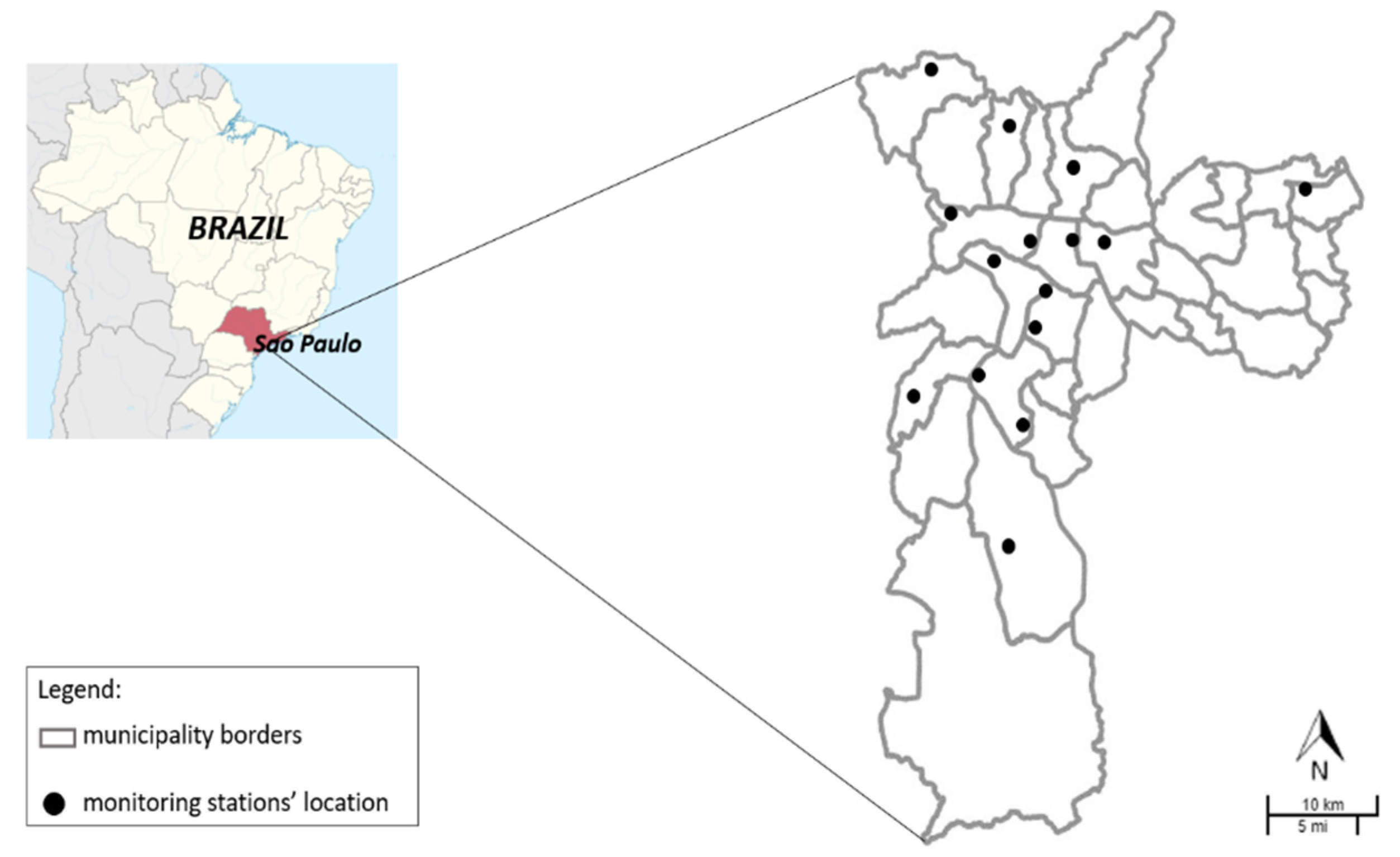
The pollutants selected for analysis were nitrogen dioxide (NO2), particulate matter with less than 10 μm (PM10) and particulate matter with less than 2.5 μm (PM2.5). Hourly atmospheric concentration data were obtained from records of QUALAR [34] for both periods. CETESB has 17 automatic monitoring stations in the municipality of Sao Paulo. Not all stations measure all pollutants. Therefore, PM10, PM2.5 and NO2 concentrations in both periods were collected, according to the availability of data from 15 monitoring stations (Figure 2), and compiled on their respective week, as previously established, to calculate the pollutants’ weekly average.
CETESB certifies that all monitoring systems of pollutants and meteorology strictly complied with the quality assurance/quality control (QA/QC) procedure established, as approved by the State Council of the Environment (CONSEMA) of Sao Paulo state [34].
The statistical analyses were performed using GraphPad Prism® 5.0 software for analysis and graphing. The data were analyzed for normality by the D’Agostino-Pearson test. As the pollutants’ concentrations behave as nonparametric variables, we used the Mann–Whitney test or Kruskal –Wallis test followed by Dunn’s post hoc test to compare the weekly average of quarantine and control periods.
The images of NO2 were detected through the Tropospheric Monitoring Instruments (TROPOMI) on-board European Space Agency (ESA) Sentinel-5 satellite, based on the Differential Optical Absorption Spectroscopy (DOAS) retrieval method in the 405–465 nm spectral range [41].
To represent the reduction in NO2 during the quarantine period, two images were captured: 25 May 2020 (4:00 pm UTC) and 21 May 2019 (3:33 pm UTC), with minimal cloud cover. The predominant wind direction data were collected from CETESB and were estimated within the limits of the municipality for both analyzed years. The measurements were performed in the south (23° 40’ 56.921” S 46° 40’ 33.884” W) and north (23° 32’ 57.48” S 46° 36’ 5.659” W) regions of Sao Paulo.
The extraction and processing of the images were performed by Sentinel Hub EO Browser, Google Earth Pro, and ImageJ. This latter software was used to convert the images from RGB to 8-bit grayscale and to quantify the mean gray value as an approach to estimate the variation of NO2 concentration on the tropospheric vertical column [42,43].
The social distancing index was made available by the telecommunications service providers through a Big Data platform that is managed by the Brazilian Association of Telecommunications Resources (ABR Telecom). According to the telecommunication service providers, the social distancing index is based on the location obtained by cell phone antennas, which “mark” a reference for the place where the cell phone “slept” between 10 pm and 2 am. During the day, a cell phone that has departed from this reference (which is variable but can reach approximately 200 m in the city of Sao Paulo) is considered out of isolation. All this processing is performed by the operator. The index is updated daily, and the operators aggregate and anonymize the data before the generation of the indexes with respect to privacy of the telephone mobile users. Thus, presenting grouped georeferenced data enables the elaboration of public policies that improve measures of social isolation to confront coronaviruses [44].
Based on air pollution reduction results for the quarantine period, the relative risk and avoided deaths attributed to each pollutant were estimated, adopting regression coefficients from epidemiological studies, a well-established method used to estimate the outcomes of air pollution on health [45,46,47,48,49,50,51,52]. The regression coefficients (β) assumed in this study were 0.0008 for PM10, 0.00405 for PM2.5, and 0.00135 for NO2-related deaths, as previously stated [52,53,54,55]. The coefficients were used to estimate the probability of mortality associated with the exposure of the pollutants, named relative risk (RR), obtained by Equation (1)
where RR is the relative risk of all-cause mortality due to air pollution; β exposure–response coefficients are related to each pollutant; and ΔX is the decrease in the pollutant concentrations (µg/m3), the difference in pollutant concentrations between the quarantine period and the equivalent period in 2018.
RR = exp [ᵝ (∆x)],
The RR values were used to calculate the attributable fraction (AF), the fraction of deaths attributable to the risk factor of PM10, PM2.5, or NO2 variation, defined in Equation (2), to estimate the avoided daily mortality during the quarantine period, based on the mean mortality in the control period.
AF = (RR − 1)/RR,
The daily mean of the all-cause mortality in the control period was calculated and multiplied by the attributable factors to estimate the all-cause mortality avoided per day during the quarantine period.
The latest update of all cause daily mortality between March 2019 and June 2019 was collected from the Brazilian Health System Database [56]. For the effects of short-term exposure to PM2.5, only all-cause mortality in people older than 30 years old was considered. The health effects caused by this pollutant justified the selection of this age group. Exposure to PM2.5 is related to hypertension, lung cancer, type 2 diabetes, and other health conditions, which are mostly observed in this age group [57,58]. For PM10 and NO2, all ages were considered. The daily data of COVID-19 deaths were obtained from the State System for Data Analysis Foundation database from 16 March 2020 to 14 June 2020 [59].
The economic valuation of health outcomes was performed by the value of statistical life (VSL) estimation, a well-known approach [60,61,62,63,64]. Considering the avoided deaths related to air pollutant emissions reduction, an economic gain is expected. However, due to the deaths caused by COVID-19, a considerable economic loss is expected.
To estimate the economic impact of the quarantine and to calculate the trade-off between mortality and economic costs, data on confirmed deaths caused by COVID-19, collected from governmental records [59], were multiplied by the VSL established value. The same calculus was used to estimate avoided deaths related to air pollutant emissions.
3. Results
3.1. Air Quality Improvement during 90 Days of COVID-19 Social Distancing
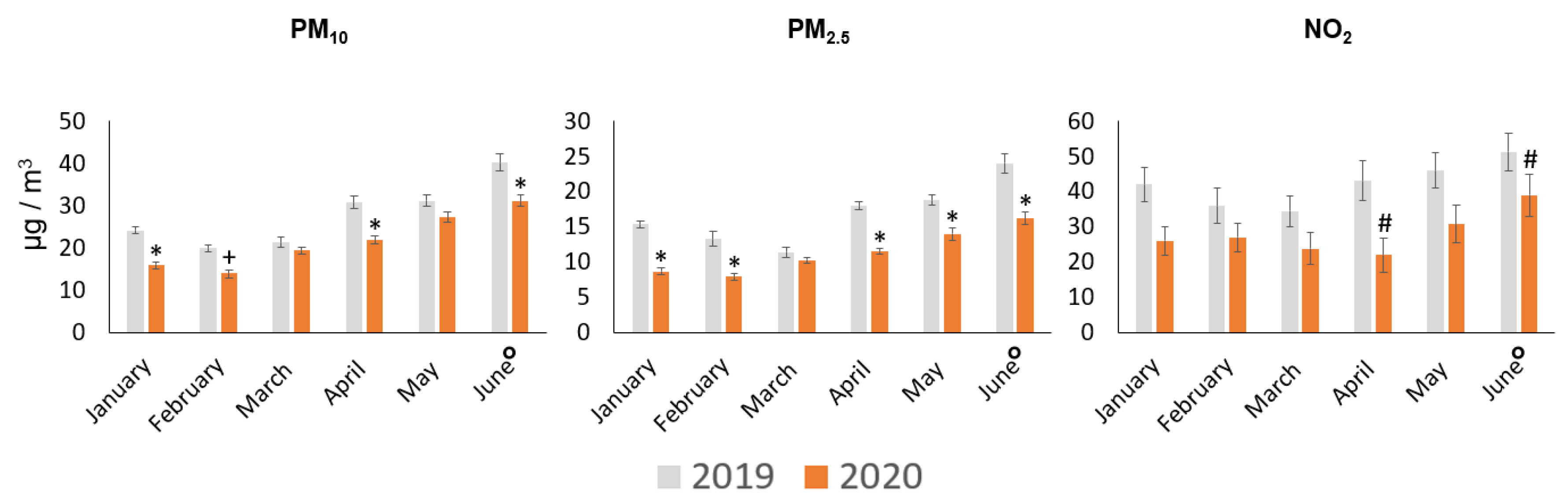
As a first-step approach, we verified the monthly records of PM10, PM2.5, and NO2 concentrations. Except for March and May, PM10 showed a significant reduction in 2020. PM2.5 also showed a significant reduction in 2020, except in March. Finally, NO2 showed a significant decrease in April and June (Figure 3).
Higher volumes of precipitation could explain the results observed for January, February, and March. In addition, the comparison between incompatible days, in terms of meteorological conditions, can affect the interpretation of the analysis. For instance, NO2 did not show a significant reduction in March and April (Figure 3). However, several studies have shown its reduction during the pandemic in different regions of the world [66,67,68].
From this initial analysis, we can conclude that the division of the analysis period on a weekly scale, considering meteorological conditions as an exclusion criterion, could provide more accurate information about the variation of pollutants.
We verified the daily records of precipitation, wind speed, and mean temperature. Comparing both periods (2019 and 2020), we observed that wind speed and mean temperature presented similar ranges. For precipitation, we detected a slight difference in a few days of the control period. Considering that precipitation is an important factor that influences the dilution and dispersion of pollutants [69,70,71,72], a 12-day control period with precipitation above 10 mm was not considered in this study. After excluding these outlier days, we observed that the means and ranges of meteorological variables were similar over the weeks of the quarantine and control periods (Table 2).
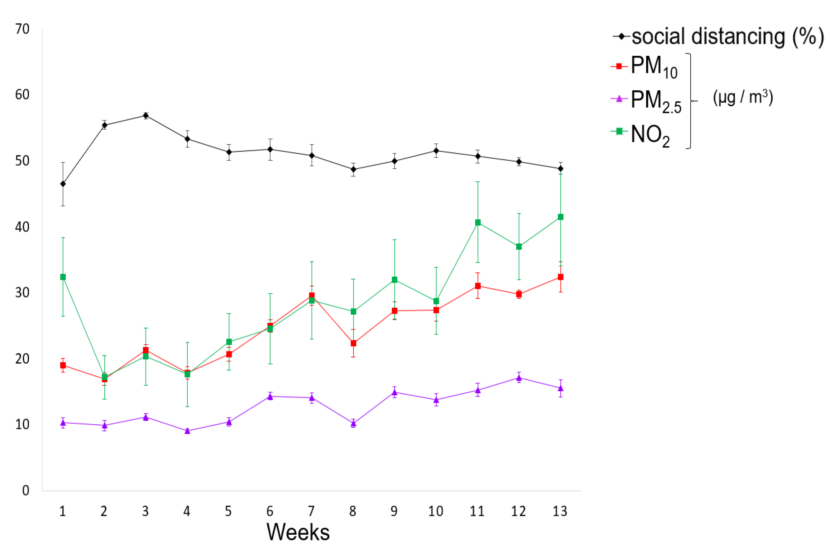
During 13 weeks of social distancing, we observed that the pollutants showed a gradual increase in concentrations over the weeks, similar to the monthly analysis. For PM10, the average concentrations ranged between 16.9 (week 2) and 32.38 µg/m3 (week 13). PM2.5 presented average concentrations varying between 9.05 (week 4) and 17.15 µg/m3 (week 12). For NO2, the average concentrations ranged between 17.21 (week 1) and 40.71 µg/m3 (week 11) (Figure 4).
The average social distancing also fluctuated, presenting the lowest index at week 1 (46.5%) and the highest between weeks 2 and 4 (55.4; 56.9 and 53.3%, respectively). In the remaining weeks, the average social distancing ranged between 51.7 and 48.7%.
The best air quality indexes for all pollutants were observed at weeks 2 and 4, with social distances above 53.3%, and the worst concentrations were detected at weeks 12 and 13, with social distances less than 50%.
From week 4 on, we also found a slackening in the social distancing accompanied by an increase in the average pollutant concentrations, quite evident for PM10 and NO2. The remaining weeks recorded at least two days, reaching six consecutive days in week 13, with less than 50% social distancing. Some factors have contributed to the reduction in social distancing, such as popular manifestations against this measure that occurred in several days, differences in federal and local governments recommendations concerning COVID-19 prevention actions, and most importantly the poor and working class who do not have alternatives in this matter, can also explain the reduction in its index and consequently the fluctuation of pollutants’ concentrations (Figure 4).
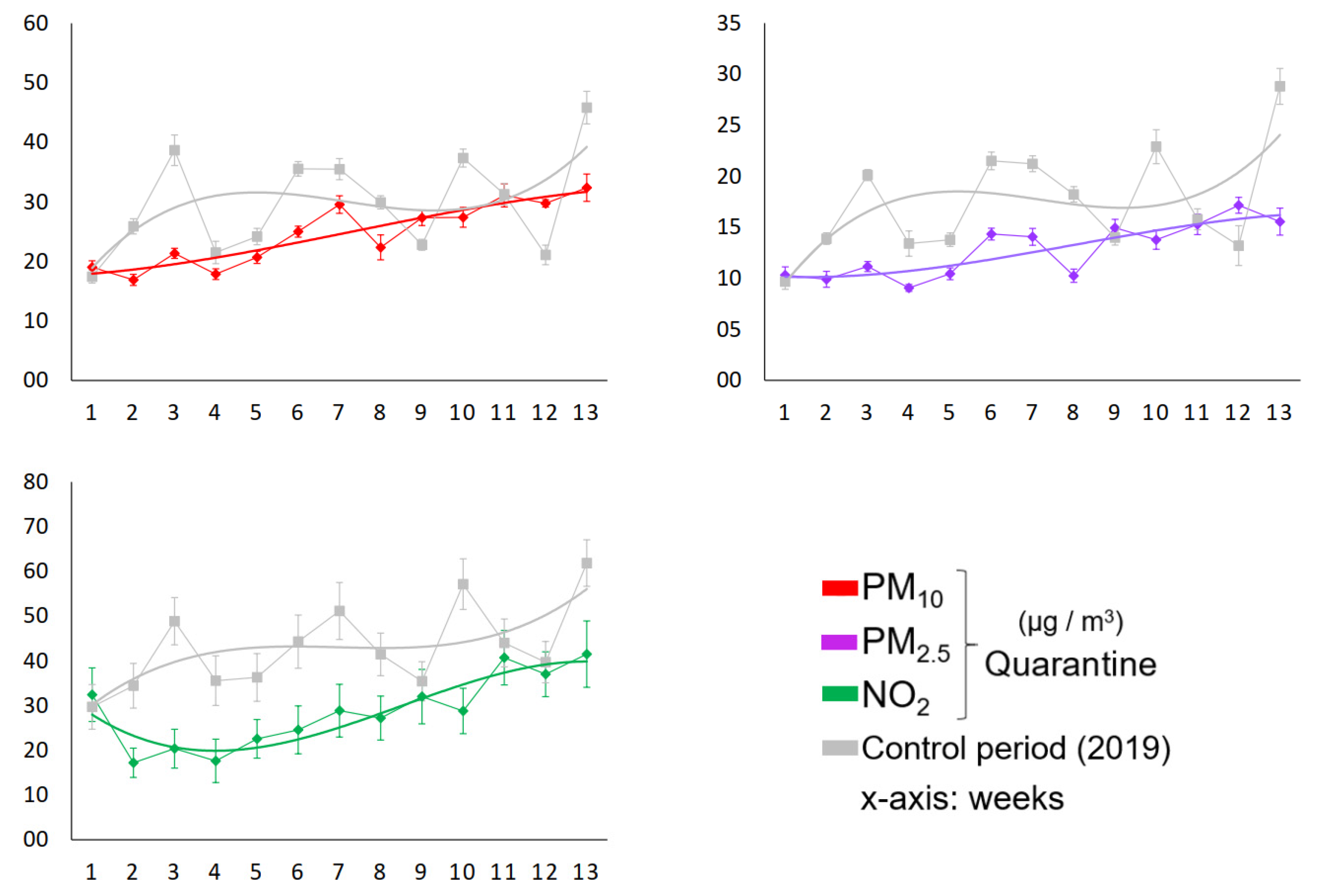
As shown in Figure 5, the comparison between the PM10 concentrations during quarantine and control periods revealed six weeks with a reduction of at least 25%, the highest reaching –45% in week 3 (p < 0.001). For PM2.5, we found eight weeks with a reduction of at least 29%, reaching –46% in week 13 (p < 0.001). The air quality improvement in terms of NO2 showed nine weeks with a reduction of at least 33%, reaching –58% in week 3 (p < 0.01).
Following PM2.5, NO2 was the best indicator of air quality in the analyzed weeks. This finding could be confirmed from the satellite images detected on 21 May 2019, and 25 May 2020, which showed an abrupt decline of 62.8% in tropospheric NO2 concentrations, represented by the variation of the red pattern (Figure 6).
3.2. Associated Health Economics Outcomes
Based on the results presented in Figure 5, we estimated the potential health and economic benefits related to pollutant reductions achieved during the analyzed weeks of quarantine. As shown in Table 3, the relative risks (RRs) were estimated to be between 0.993 and 1.013 for PM10, 0.996 and 1.055 for PM2.5, and 0.996 and 1.039 for NO2. Thus, the attributable factors (AF) ranged 0.2–0.8% for PM10, 0.9–3.2% for PM2.5, and 4–6.9% for NO2. As expected, because NO2 presented the greatest levels of reduction compared to the control period, its weekly RR and AF values were also higher in relation to other analyzed pollutants.
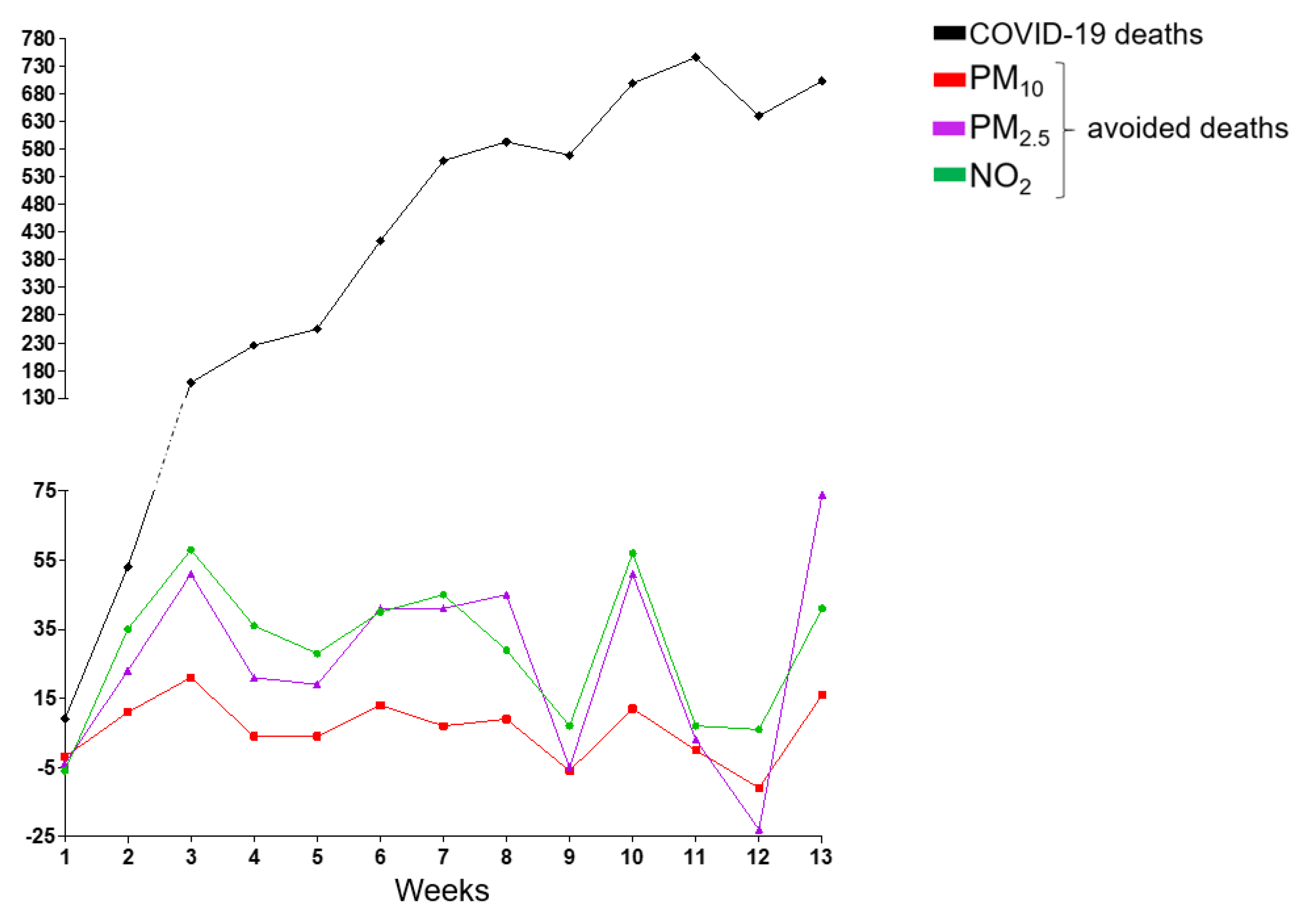
Therefore, concomitant with the increase in the number of deaths from COVID-19 infection, which reached 5623 on the last day of this analysis, the decrease in PM10, PM2.5, and NO2 concentration levels prevented 78,337 and 387 premature deaths, respectively, in Sao Paulo city (Figure 7).
Given the monetary value for the observed health outcomes from the analyzed improvement of pollutant concentrations by the VSL approach, a well-known and widely used method [65,73], we applied the economic valuation of deaths caused by COVID-19 and of the avoided deaths due to the reduction in short-term exposure to PM10, PM2.5, and NO2 (Table 4).
During the analyzed weeks of the quarantine period in Sao Paulo city, the deaths caused by COVID-19 accounted for an economic health loss of approximately US $10.5 billion. On the other hand, we can consider a potential economic health benefit in terms of the prevented premature deaths related to the observed improvement in air quality. Thus, we estimated that the expressive number of avoided deaths due to PM10, PM2.5, and NO2 reductions can represent an economy of approximately US $720 million, considering the results of NO2, the best air quality indicator observed.
4. Discussion
In a tightly connected and integrated world, the impacts of emerging infectious diseases can be devastating, causing large-scale mortality and morbidity, as we are observing over the days of this global outbreak. However, the adverse effects go beyond, and the size and persistence of the economic impacts of the ongoing COVID-19 pandemic are still uncertain, and our findings raise intriguing questions.
On the one hand, we estimated the economic health loss associated with deaths related to COVID-19 in Sao Paulo city, which was exceedingly raised, even before reaching the important goal of flattening the curve of coronavirus infections, which makes us wonder about the efficiency of the applied public policies and the commitment of the strategies of controlling the pandemic and population’s commitment to comply with social distancing. On the other hand, we observed that the epidemic control actions were closely related to the improvement of air quality; due to the major source of air pollution in the region, the emissions from vehicle exhaust were significantly reduced.
The quarantine and cities in shutdown have also caused a supplementary effect, the improvement of air quality, which was observed in different regions of the world, such as India, China, Italy, France, and United States [66,67,74]. In Rio de Janeiro, Brazil, a study showed that the confinement of the population between March and April caused a reduction in road traffic and economic activities and led to a significant decrease in CO (between 37.0 and 43.6%) and NO2 (between 24.1 and 32.9%) levels and a non-significant reduction in PM10 concentrations [75].
Regarding NO2 and particulate matter, our findings showed that, in Sao Paulo, the impacts on its concentrations were more significant. During 16 March and 14 June 2020, NO2 decreased to 33%, reaching 58%, the decrease in PM10 ranged between 25 and 45%, and the levels of PM2.5 decreased between 29 and 46% in comparison to the control period in 2019.
Air quality improvement could also be observed by satellite images worldwide. A dramatic reduction in air pollution over China during February 2020 accounted for over 30% less in NO2 levels compared to early January when power plants were operating at normal levels. In addition, the study also estimated a reduction of CO2 emissions by 25% [66]. Xu et al. (2020) showed that from January to March 2020, the decrease in NO2 concentration was of great significance and much higher than other pollutants, such as PM10 and PM2.5 [68]. Moreover, Anjum (2020) also showed, from satellite images, a remarkable reduction of air pollution in Italy, France, and the USA [67].
Our results corroborate these findings since we also showed a significant reduction in NO2 concentration in Sao Paulo city, which was greater than the other analyzed pollutants, confirmed by the abrupt decline of 62.8% in tropospheric NO2 concentrations also observed by satellite images.
Human activities do not change only the atmosphere with the emission of pollutants or only the climate system with the emission of greenhouse gases; the consequences are systemic since they can directly affect human health, socioeconomic, and political stability. Emissions of air pollutants related to the exacerbation of the prevalence of cardiorespiratory diseases, type 2 diabetes, and mental disorders; land use modification associated with deforestation that modifies host/vector interactions, elevates disease risk, and drives wildlife zoonotic disease emergence; and mega-trends in climate accompanied by extreme weather conditions make the population increasingly vulnerable. These conditions can cause several socioeconomic impacts, such as morbidities, mortality, migration, poverty exacerbation, and violent conflict, affecting people of all ages and all nationalities [29,76,77].
In this context, the current global crisis we are experiencing goes beyond showing that environmental degradation is closely related to human resilience. In times of crisis, borders do not matter, showing the importance of cooperation and engagement of governments and all the people to work together for a common purpose and solution.
Foregone income related to laid-off workers or unable to work, disruption of supply chains, restrictions on international travel enforced by governments, and unprecedented consequences on stock markets are examples of already observed economic and social impacts. Individualities and structural differences of each country make forecasts difficult; however, there are some published estimates. According to Fernandes (2020), for Brazil, the GDP growth in 2020, assuming shutdown lasts three months, can reach −4.0% [from −5.9% to −2.1%]. Moreover, according to the OECD, global GDP growth is projected to slow from 2.9% in 2019 to 2.4% in 2020 [78,79,80]. The COVID-19 pandemic has hit underserved populations and communities of color particularly hard, exacerbating longstanding health disparities in Brazil. This fact can be observed in Sao Paulo municipality, which districts of poorer areas have been suffering most of the cases of COVID-19.
Politicians and some businessmen are against social distancing measures due to the impact on the economy, claiming that the virus is less harmful than presented; they do not value life. Life is more valuable than the economy—there is no need to have good economic indicators if the population dies. Nevertheless, there will be economic effects of the distance measures and the impacts on the mental health of the populations affected by them. In addition to anxiety due to fear of the disease, there are effects of prolonged quarantine for several weeks faced by a huge number of people around the world.
An impact assessment evaluation can consider the exposure to a multi-pollutant mixture. Adding pollutant-specific effects may be justified when levels of the specific pollutants are clearly not correlated. However, this approach would result in an overestimated analysis due to uncertainties about the contributions of each pollutant to the health effect [81,82].
In this research, we estimated the health effects concerning a reduction in PM10, PM2.5 and NO2 concentrations. Thus, to avoid a biased analysis, we considered, in the health economic evaluation, the outcomes of NO2, the best air quality indicator observed. Accordingly, our results showed that air quality improvement contributed to a substantial fraction of the avoided deaths associated with significant monetized health co-benefits, signaling that governments have the capability to improve air quality through policy measures.
We found that the decrease in PM10, PM2.5, and NO2 concentration levels could prevent 78,337 and 387 premature deaths, respectively, corresponding to an economy of approximately US $720 million and providing evidence for policy making by the quantification and monetization of air pollution-related health effects. This is a tool for environmental planning purposes since the monetized value of the avoided premature mortality typically dominates the calculated benefits of air pollution regulations.
The consideration of exclusively NO2 abatement in the quarantine period is a conservative simplification. This constraint may have biased our estimation downwards. If we add the effect of PM2.5 and PM10, we double the impact of prevented deaths due to air pollution, meaning a saving of US $1.5 billion. Considering the maintenance of these mobility patterns in the new “business as usual” (BAU) COVID-19 era, in a 10-year period, this savings would achieve approximately US $60 billion. Both health and economic gains associated with air pollution reductions give a positive perspective of the efforts towards keeping air pollution reduced even after the pandemic.
Unprecedented challenge demands an unprecedented response. Thus, shifting the BAU approach of life will be the most important and mandatory step to prevent future adverse events. For that, resilience is indispensable for facing new problems and challenges in our increasingly globalized world. The COVID-19 pandemic, forcing a drastic change in the BAU way of life, offers a unique scenario to take the opportunity during the crisis to move toward a more sustainable society and economy, in terms of speeding up the transition of make cities more inclusive, developing urban resilience, improving preventive health measures, and implementing green strategies for economics, especially for transport and energy sectors, since they are major contributors to the degradation of global air quality [20,33,83,84].
In this sense, our analysis presents an estimate of what could be achieved if effective measures would be taken towards air pollution emissions control in an urban center of a developing country, such as Sao Paulo. The implementation of permanent or partial home-office jobs, dynamization of e-commerce, as well as improvement of energy efficiency, support of a low-carbon economy, and investments in cleaner transportation solutions are some recommendations for sustainable procedures that can diminish air pollution emissions in megacities, providing a transition to urban resilience and sustainability.
5. Conclusions
We found that, during 90 days of COVID-19 social distancing in Sao Paulo city, Brazil, 5623 deaths occurred due to this new disease estimated in an economic health loss of US $10.5 billion. In contrast, we observed a significant air quality improvement. During the analyzed weeks, the decreases in PM2.5, PM10, and NO2 levels reached 45%, 46%, and 58% reductions, respectively, in comparison to the control period in 2019. The positive impact on air quality in terms of PM2.5, PM10, and NO2 concentrations avoided 78,337 and 387 premature deaths, respectively, and prevented approximately US $720 million on health costs, considering the results of NO2, the best air quality indicator observed.
Our study faced some limitations. First, in addition to the reduced number of deaths due to air pollution, we should consider that there are other benefits attributable to the reduction in air pollution itself and could also have positive benefits in reducing preventable noncommunicable diseases [85,86]. Thus, a more comprehensive analysis should contemplate other health outcomes, such as the reductions in hospitalizations due to cardiorespiratory diseases. Second, meteorological data were collected and used as a criterion for selected days of the control period to ensure that the analysis was not carried out on incompatible days in terms of the meteorological similarity of both periods analyzed, minimizing the influence of these factors on pollutant dispersion. In this sense, an air quality dispersion modeling approach could be usefully explored in further future researches.
These findings have significant implications for understanding how important it is to improve the strategies for sustainable practices in urban centers, especially with regard to air pollution mitigation actions. Furthermore, we highlight the crucial role of appropriately allocating investments and adopting efficient measures to protect human health both during and after the COVID-19 global health crisis.
Author Contributions
Conceptualization, S.G.E.K.M. and D.D.; formal analysis, D.D., M.V.d.C., and S.G.E.K.M.; writing—original draft preparation, D.D., M.V.d.C., and S.G.E.K.M.; writing—review and editing, D.D., M.V.d.C., and S.G.E.K.M.; supervision, S.G.E.K.M. All authors have read and agreed to the published version of the manuscript.
Funding
Supported by Grant Number 1808529 from the Coordenação de Aperfeiçoamento de Pessoal de Nível Superior (CAPES). Supported by Grant Number 2018/26193-3 from the Fundação de Amparo à Pesquisa do Estado de São Paulo (FAPESP).
Acknowledgments
The authors are grateful to the Academic Editor Idiano D’Adamo and Etta Shen for all support provided.
Conflicts of Interest
The authors declare no conflict of interest.
References
- Brida, M.; Chessa, M.; Gu, H.; Gatzoulis, M.A. The globe on the spotlight: Coronavirus disease 2019 (Covid-19). Int. J. Cardiol. 2020, 310, 170–172. [Google Scholar] [CrossRef] [PubMed]
- Tu, H.; Tu, S.; Gao, S.; Shao, A.; Sheng, J. Current epidemiological and clinical features of COVID-19; a global perspective from China. J. Infect. 2020, 81, 1–9. [Google Scholar] [CrossRef] [PubMed]
- Martini, M.; Gazzaniga, V.; Bragazzi, N.L.; Barberis, I. The Spanish Influenza Pandemic: A lesson from history 100 years after 1918. J. Prev. Med. Hyg. 2019, 60, E64–E67. [Google Scholar] [CrossRef]
- Dhama, K.; Verma, A.K.; Rajagunala, S.; Deb, R.; Karthik, K.; Kapoor, S.M.; Tiwari, R.; Panwar, P.K.; Chakrabort, S. Swine flu is back again: A review. Pakistan J. Biol. Sci. 2012, 15, 1001–1009. [Google Scholar] [CrossRef] [Green Version]
- World Health Organization. Influenza Updates; World Health Organization: Geneva, Switzerland, 2020; Available online: https://www.who.int/influenza/surveillance_monitoring/updates/en/ (accessed on 18 June 2020).
- Centers for Disease Control and Prevention. Influenza (Flu). 2009 H1N1 Pandemic; Centers for Disease Control and Prevention: Atlanta, GA, USA, 2009. Available online: https://www.cdc.gov/flu/pandemic-resources/2009-h1n1-pandemic.html (accessed on 18 June 2020).
- Bradley, K.C.; Jones, C.A.; Tompkins, S.M.; Tripp, R.A.; Russell, R.J.; Gramer, M.R.; Heimburg-Molinaro, J.; Smith, D.F.; Cummings, R.D.; Steinhauer, D.A. Comparison of the receptor binding properties of contemporary swine isolates and early human pandemic H1N1 isolates (Novel 2009 H1N1). Virology 2011, 413, 169–182. [Google Scholar] [CrossRef] [PubMed] [Green Version]
- Chowell, G.; Ammon, C.E.; Hengartner, N.W.; Hyman, J.M. Estimation of the reproductive number of the Spanish flu epidemic in Geneva, Switzerland. Vaccine 2006, 24, 6747–6750. [Google Scholar] [CrossRef]
- World Health Organization. Coronavirus Disease (COVID-19) Dashboard; World Health Organization: Geneva, Switzerland, 2020; Available online: https://covid19.who.int/ (accessed on 18 June 2020).
- Velavan, T.P.; Meyer, C.G. The COVID-19 epidemic. Trop. Med. Int. Health 2020, 25, 278–280. [Google Scholar] [CrossRef] [Green Version]
- Candido, D.D.S.; Watts, A.; Abade, L.; Kraemer, M.U.G.; Pybus, O.G.; Croda, J.; de Oliveira, W.; Khan, K.; Sabino, E.C.; Faria, N.R. Routes for COVID-19 importation in Brazil. J. Travel Med. 2020, 27. [Google Scholar] [CrossRef] [PubMed] [Green Version]
- Singhal, T. A review of coronavirus disease-2019 (COVID-19). Indian J. Pediatr. 2020, 87, 281–286. [Google Scholar] [CrossRef] [Green Version]
- Ahmed, K.; Hayat, S.; Dasgupta, P. Global challenges to urology practice during the COVID-19 pandemic. BJU Int. 2020. [Google Scholar] [CrossRef]
- Rothan, H.A.; Byrareddy, S.N. The epidemiology and pathogenesis of coronavirus disease (COVID-19) outbreak. J. Autoimmun. 2020, 109, 102433. [Google Scholar] [CrossRef] [PubMed]
- Lake, M.A. What we know so far: COVID-19 current clinical knowledge and research. Clin. Med. (Northfield. Il) 2020, 20, 124–127. [Google Scholar] [CrossRef] [PubMed] [Green Version]
- Conticini, E.; Frediani, B.; Caro, D. Can atmospheric pollution be considered a co-factor in extremely high level of SARS-CoV-2 lethality in northern Italy? Environ. Pollut. 2020, 261, 114465. [Google Scholar] [CrossRef] [PubMed]
- Frontera, A.; Martin, C.; Vlachos, K.; Sgubin, G. Regional air pollution persistence links to COVID-19 infection zoning. J. Infect. 2020, 81, 318–356. [Google Scholar] [CrossRef]
- Tavella, R.A.; da Silva Júnior, F.M. COVID-19 and air pollution: What do we know so far? Vittalle–Rev. Ciências da Saúde 2020, 1, 22–31. [Google Scholar] [CrossRef]
- Wu, X.; Nethery, R.C.; Sabath, B.M.; Braun, D.; Dominici, F. Exposure to air pollution and COVID-19 mortality in the United States: A nationwide cross-sectional study. medRxiv 2020. [Google Scholar] [CrossRef] [Green Version]
- Urrutia-Pereira, M.; Mello-da-Silva, C.A.; Solé, D. COVID-19 and air pollution: A dangerous association? Allergol. Immunopathol. (Madrid) 2020. [Google Scholar] [CrossRef]
- Brazilian Institute of Statistics and Geography. Estimativa da População-Diretoria de Pesquisas, Coordenação de População e Indicadores Sociais; Brazilian Institute of Statistics and Geography: Rio de Janeiro, Brasil, 2018. Available online: https://www.ibge.gov.br/cidades-e-estados.html (accessed on 18 June 2020).
- Companhia Ambiental do Estado de São Paulo. Qualidade do ar no Estado de São Paulo; Companhia Ambiental do Estado de São Paulo: São Paulo, Brasil, 2019. Available online: https://cetesb.sp.gov.br/ar/publicacoes-relatorios/ (accessed on 18 June 2020).
- Andrade, M.F.; Kumar, P.; de Freitas, E.D.; Ynoue, R.Y.; Martins, J.; Martins, L.D.; Nogueira, T.; Perez-Martinez, P.; de Miranda, R.M.; Albuquerque, T.; et al. Air quality in the megacity of São Paulo: Evolution over the last 30 years and future perspectives. Atmos. Environ. 2017, 159, 66–82. [Google Scholar] [CrossRef] [Green Version]
- Sao Paulo Transit State Department. São Paulo Vehicle Fleet; Sao Paulo Transit State Department: Sao Paulo, Brasil, 2011. Available online: https://www.detran.sp.gov.br/ (accessed on 18 June 2020).
- IEMA. Inventário De Emissões Atmosféricas Do Transporte Rodoviário De Passageiros No Município De São Paulo; IEMA: Sao Paulo, Brasil, 2020. Available online: http://emissoes.energiaeambiente.org.br/graficos (accessed on 18 June 2020).
- Scovronick, N.; França, D.; Alonso, M.; Almeida, C.; Longo, K.; Freitas, S.; Rudorff, B.; Wilkinson, P. Air quality and health impacts of future ethanol production and use in São Paulo State, Brazil. Int. J. Environ. Res. Public Health 2016, 13, 695. [Google Scholar] [CrossRef] [Green Version]
- Abe, K.; Miraglia, S. Health Impact assessment of air pollution in São Paulo, Brazil. Int. J. Environ. Res. Public Health 2016, 13, 694. [Google Scholar] [CrossRef] [Green Version]
- Leirião, L.F.L.; Debone, D.; Pauliquevis, T.; Rosário, N.M.É.; Miraglia, S.G.E.K. Environmental and public health effects of vehicle emissions in a large metropolis: Case study of a truck driver strike in Sao Paulo, Brazil. Atmos. Pollut. Res. 2020. [Google Scholar] [CrossRef]
- Rizzoli, A.; Tagliapietra, V.; Cagnacci, F.; Marini, G.; Arnoldi, D.; Rosso, F.; Rosà, R. Parasites and wildlife in a changing world: The vector-host-pathogen interaction as a learning case. Int. J. Parasitol. Parasites Wildl. 2019, 9, 394–401. [Google Scholar] [CrossRef] [PubMed]
- Allen, T.; Murray, K.A.; Zambrana-Torrelio, C.; Morse, S.S.; Rondinini, C.; Di Marco, M.; Breit, N.; Olival, K.J.; Daszak, P. Global hotspots and correlates of emerging zoonotic diseases. Nat. Commun. 2017, 8, 1124. [Google Scholar] [CrossRef]
- Guo, F.; Bonebrake, T.C.; Gibson, L. Land-use change alters host and vector communities and may elevate disease risk. Ecohealth 2019, 16, 647–658. [Google Scholar] [CrossRef] [PubMed]
- Loh, E.H.; Zambrana-Torrelio, C.; Olival, K.J.; Bogich, T.L.; Johnson, C.K.; Mazet, J.A.K.; Karesh, W.; Daszak, P. Targeting transmission pathways for emerging zoonotic disease surveillance and control. Vector Borne Zoonotic Dis. 2015, 15, 432–437. [Google Scholar] [CrossRef] [Green Version]
- D’Adamo, I.; Falcone, P.M.; Martin, M.; Rosa, P. A Sustainable revolution: Let’s go sustainable to get our globe cleaner. Sustainability 2020, 12, 4387. [Google Scholar] [CrossRef]
- Companhia Ambiental do Estado de São Paulo. QUALAR. Sistema de Informações da Qualidade do Ar; CETESB: São Paulo, Brasil, 2020. Available online: https://qualar.cetesb.sp.gov.br/qualar/home.do (accessed on 18 June 2020).
- AGRITEMPO. Brazilian Agro-Meteorological Monitoring System; AGRITEMPO: Rio de Janeiro, Brasil, 2019. Available online: https://www.agritempo.gov.br/agritempo/index.jsp (accessed on 18 June 2020).
- Sánchez-Ccoyllo, O.R.; de Fátima Andrade, M. The influence of meteorological conditions on the behavior of pollutants concentrations in São Paulo, Brazil. Environ. Pollut. 2002, 116, 257–263. [Google Scholar] [CrossRef]
- Zeri, M.; Carvalho, V.S.B.; Cunha-Zeri, G.; Oliveira-Júnior, J.F.; Lyra, G.B.; Freitas, E.D. Assessment of the variability of pollutants concentration over the metropolitan area of São Paulo, Brazil, using the wavelet transform. Atmos. Sci. Lett. 2016, 17, 87–95. [Google Scholar] [CrossRef] [Green Version]
- Carneseca, E.C.; Achcar, J.A.; Martinez, E.Z. Association between particulate matter air pollution and monthly inhalation and nebulization procedures in Ribeirão Preto, São Paulo State, Brazil. Cad. Saude Publica 2012, 28, 1591–1598. [Google Scholar] [CrossRef] [Green Version]
- Tanzer-Gruener, R.; Li, J.; Eilenberg, S.R.; Robinson, A.L.; Presto, A.A. Impacts of modifiable factors on ambient air pollution: A case study of COVID-19 shutdowns. Environ. Sci. Technol. Lett. 2020, 7, 554–559. [Google Scholar] [CrossRef]
- Freitas, E.D.; Ibarra-Espinosa, S.A.; Gavidia-Calderón, M.E.; Rehbein, A.; Abou Rafee, S.A.; Martins, J.A.; Martins, L.D.; Santos, U.P.; Ning, M.F.; Andrade, M.F. Mobility restrictions and air quality under COVID-19 pandemic in São Paulo, Brazil. Earth Sci. 2020. [Google Scholar] [CrossRef]
- Wang, C.; Wang, T.; Wang, P.; Rakitin, V. Comparison and validation of TROPOMI and OMI NO2 Observations over China. Atmosphere (Basel) 2020, 11, 636. [Google Scholar] [CrossRef]
- Lopez, J.; Branch, J.W.; Chen, G. Line-based image segmentation method: A new approach to segment VHSR remote sensing images automatically. Eur. J. Remote Sens. 2019, 52, 613–631. [Google Scholar] [CrossRef] [Green Version]
- Ciobotaru, A.-M.; Andronache, I.; Ahammer, H.; Radulovic, M.; Peptenatu, D.; Pintilii, R.-D.; Drăghici, C.-C.; Marin, M.; Carboni, D.; Mariotti, G.; et al. Application of Fractal and gray-level co-occurrence matrix indices to assess the forest dynamics in the curvature Carpathians—Romania. Sustainability 2019, 11, 6927. [Google Scholar] [CrossRef] [Green Version]
- Sistema de Monitoramento Inteligente do Governo de São Paulo. Available online: https://www.saopaulo.sp.gov.br/coronavirus/isolamento/ (accessed on 27 June 2020).
- Abe, K.C.; dos Santos, G.M.S.; Coêlho, M.; de Sousa, Z.S.; Miraglia, S.G.E.K. PM10 exposure and cardiorespiratory mortality–estimating the effects and economic losses in São Paulo, Brazil. Aerosol Air Qual. Res. 2018, 18, 3127–3133. [Google Scholar] [CrossRef] [Green Version]
- Bell, M.L.; Ebisu, K.; Peng, R.D.; Samet, J.M.; Dominici, F. Hospital admissions and chemical composition of fine particle air pollution. Am. J. Respir. Crit. Care Med. 2009, 179, 1115–1120. [Google Scholar] [CrossRef]
- Hemminki, K.; Pershagen, G. Cancer risk of air pollution: Epidemiological evidence. Environ. Health Perspect. 1994, 102, 187–192. [Google Scholar] [CrossRef] [PubMed]
- Hoek, G.; Brunekreef, B.; Goldbohm, S.; Fischer, P.; van den Brandt, P.A. Association between mortality and indicators of traffic-related air pollution in the Netherlands: A cohort study. Lancet 2002, 360, 1203–1209. [Google Scholar] [CrossRef] [Green Version]
- Jerrett, M.; Burnett, R.T.; Ma, R.; Pope, C.A.; Krewski, D.; Newbold, K.B.; Thurston, G.; Shi, Y.; Finkelstein, N.; Calle, E.E.; et al. Spatial analysis of air pollution and mortality in Los Angeles. Epidemiology 2005, 16, 727–736. [Google Scholar] [CrossRef] [PubMed]
- Nyhan, M.M.; Kloog, I.; Britter, R.; Ratti, C.; Koutrakis, P. Quantifying population exposure to air pollution using individual mobility patterns inferred from mobile phone data. J. Expo. Sci. Environ. Epidemiol. 2019, 29, 238–247. [Google Scholar] [CrossRef] [PubMed]
- Ostro, B.; Malig, B.; Broadwin, R.; Basu, R.; Gold, E.B.; Bromberger, J.T.; Derby, C.; Feinstein, S.; Greendale, G.A.; Jackson, E.A.; et al. Chronic PM2.5 exposure and inflammation: Determining sensitive subgroups in mid-life women. Environ. Res. 2014, 132, 168–175. [Google Scholar] [CrossRef] [PubMed] [Green Version]
- Mudu, P.; Gapp, C.; Dunbar, M. AirQ+ 1.0 Example of Calculations; World Health Organization: Geneva, Switzerland, 2016. [Google Scholar]
- Mead, R.W.; Brajer, V. Rise of the Automobiles: The costs of increased NO 2 pollution in China’s changing urban environment. J. Contemp. China 2006, 15, 349–367. [Google Scholar] [CrossRef]
- Ostro, B.; Prüss-Ustün, A.; Campbell-lendrum, D.; Corvalán, C.; Woodward, A. Outdoor Air Pollution: Assessing the Environmental Burden of Disease at National and Local Levels; World Health Organization: Geneva, Switzerland, 2004; pp. 1–54. ISBN 92 4 159146 3. [Google Scholar]
- Debone, D.; Leirião, L.F.L.; Miraglia, S.G.E.K. Air quality and health impact assessment of a truckers’ strike in Sao Paulo state, Brazil: A case study. Urban. Clim. 2020, 34, 100687. [Google Scholar] [CrossRef]
- DATASUS. Brazilian Health System Database (TABNET). Available online: http://datasus.saude.gov.br/informacoes-de-saude/tabnet (accessed on 18 June 2020).
- Coogan, P.F.; White, L.F.; Yu, J.; Burnett, R.T.; Seto, E.; Brook, R.D.; Palmer, J.R.; Rosenberg, L.; Jerrett, M. PM2. 5 and diabetes and hypertension incidence in the Black Women’s Health Study. Epidemiology 2016, 27, 202. [Google Scholar] [PubMed] [Green Version]
- Li, R.; Zhou, R.; Zhang, J. Function of PM2. 5 in the pathogenesis of lung cancer and chronic airway inflammatory diseases. Oncol. Lett. 2018, 15, 7506–7514. [Google Scholar] [PubMed] [Green Version]
- SEADE. State Data Analysis System. Available online: https://www.seade.gov.br/institucional/ (accessed on 27 June 2020).
- Alberini, A.; Hunt, A.; Markandya, A. Willingness to pay to reduce mortality risks: Evidence from a three-country contingent valuation study. Environ. Resour. Econ. 2006, 33, 251–264. [Google Scholar] [CrossRef] [Green Version]
- Ding, D.; Xing, J.; Wang, S.; Liu, K.; Hao, J. Estimated contributions of emissions controls, meteorological factors, population growth, and changes in baseline mortality to reductions in ambient PM2.5 and PM2.5-related mortality in China, 2013–2017. Environ. Health Perspect. 2019, 127, 067009. [Google Scholar] [CrossRef]
- Ran, T.; Nurmagambetov, T.; Sircar, K. Economic implications of unintentional carbon monoxide poisoning in the United States and the cost and benefit of CO detectors. Am. J. Emerg. Med. 2018, 36, 414–419. [Google Scholar] [CrossRef]
- Robinson, L.A. Estimating the values of mortality risk reductions in low-and middle-income countries. J. Benefit Cost Anal. 2017, 8, 205–214. [Google Scholar] [CrossRef] [Green Version]
- Wolfe, P.; Davidson, K.; Fulcher, C.; Fann, N.; Zawacki, M.; Baker, K.R. Monetized health benefits attributable to mobile source emission reductions across the United States in 2025. Sci. Total Environ. 2019, 650, 2490–2498. [Google Scholar] [CrossRef]
- Roy, R.; Braathen, N.A. The Rising Cost of Ambient Air Pollution thus far in the 21st Century: Results from the BRIICS and the OECD Countries; OECD Environ. Working Paper; OECD: Paris, France, 2017; Available online: https://0-www-oecd--ilibrary-org.brum.beds.ac.uk/ (accessed on 27 June 2020).
- Isaifan, R.J. The dramatic impact of Coronavirus outbreak on air quality: Has it saved as much as it has killed so far? Glob. J. Environ. Sci. Manag. 2020, 6, 275–288. [Google Scholar]
- Anjum, N.A. Good in the worst: COVID-19 restrictions and ease in global air pollution. 2020; preprint. [Google Scholar] [CrossRef]
- Xu, K.; Cui, K.; Young, L.-H.; Hsieh, Y.-K.; Wang, Y.-F.; Zhang, J.; Wan, S. Impact of the COVID-19 event on air quality in central China. Aerosol Air Qual. Res. 2020, 20, 915–929. [Google Scholar] [CrossRef] [Green Version]
- Chou, S.C.; Bustamante, J.F.; Gomes, J.L. Evaluation of Eta Model seasonal precipitation forecasts over South America. Nonlinear Process. Geophys. 2005, 12, 537–555. [Google Scholar] [CrossRef] [Green Version]
- Pellon de Miranda, F.; Marmol, A.M.Q.; Pedroso, E.C.; Beisl, C.H.; Welgan, P.; Morales, L.M. Analysis of RADARSAT-1 data for offshore monitoring activities in the Cantarell Complex, Gulf of Mexico, using the unsupervised semivariogram textural classifier (USTC). Can. J. Remote Sens. 2004, 30, 424–436. [Google Scholar] [CrossRef]
- Ramis, J.E.; dos Santos, E.A. The impact of thermal comfort in the perceived level of service and energy costs of three Brazilian airports. J. Transp. Lit. 2013, 7, 192–206. [Google Scholar] [CrossRef] [Green Version]
- Yu, K.-P. Enhancement of the deposition of ultrafine secondary organic aerosols by the negative air ion and the effect of relative humidity. J. Air Waste Manag. Assoc. 2012, 62, 1296–1304. [Google Scholar] [CrossRef] [Green Version]
- Markandya, A.; Sampedro, J.; Smith, S.J.; Van Dingenen, R.; Pizarro-Irizar, C.; Arto, I.; González-Eguino, M. Health co-benefits from air pollution and mitigation costs of the Paris Agreement: A modelling study. Lancet Planet. Heal. 2018, 2, e126–e133. [Google Scholar] [CrossRef] [Green Version]
- Sharma, S.; Zhang, M.; Anshika; Gao, J.; Zhang, H.; Kota, S.H. Effect of restricted emissions during COVID-19 on air quality in India. Sci. Total Environ. 2020, 728, 138878. [Google Scholar] [CrossRef]
- Dantas, G.; Siciliano, B.; França, B.B.; da Silva, C.M.; Arbilla, G. The impact of COVID-19 partial lockdown on the air quality of the city of Rio de Janeiro, Brazil. Sci. Total Environ. 2020, 729, 139085. [Google Scholar] [CrossRef]
- Grande, G.; Ljungman, P.L.S.; Eneroth, K.; Bellander, T.; Rizzuto, D. Association between cardiovascular disease and long-term exposure to air pollution with the risk of dementia. JAMA Neurol. 2020. [Google Scholar] [CrossRef] [Green Version]
- Watts, N.; Amann, M.; Arnell, N.; Ayeb-Karlsson, S.; Belesova, K.; Berry, H.; Bouley, T.; Boykoff, M.; Byass, P.; Cai, W.; et al. The 2018 report of the Lancet Countdown on health and climate change: Shaping the health of nations for centuries to come. Lancet 2018, 392, 2479–2514. [Google Scholar] [CrossRef]
- Baldwin, R.E.; di Mauro, W. Mitigating the COVID Economic Crisis; CEPR Press: Washington, DC, USA, 2020; Available online: https://iheid.tind.io/record/298223 (accessed on 18 June 2020).
- OECD. OECD Economic Outloo; OECD: Paris, France, 2020; Volume 2020, ISBN 9789264524156. [Google Scholar]
- Fernandes, N. Economic effects of coronavirus outbreak (COVID-19) on the world economy. SSRN Electron. J. 2020. [Google Scholar] [CrossRef]
- WHO. Quantification of Health Effects of Exposure to Air Pollution: Report on a WHO Working Group, Bilthoven, Netherlands 20–22 November 2000; World Health Organization: Geneva, Switzerland, 2000; Available online: https://apps.who.int/iris/handle/10665/108463 (accessed on 18 June 2020).
- Blangiardo, M.; Pirani, M.; Kanapka, L.; Hansell, A.; Fuller, G. A hierarchical modelling approach to assess multi pollutant effects in time-series studies. PLoS ONE 2019, 14, e0212565. [Google Scholar] [CrossRef] [PubMed] [Green Version]
- Koehl, A. Urban transport and COVID-19: Challenges and prospects in low-and middle-income countries. Cities Heath 2020, 4, 1–6. [Google Scholar]
- D’Adamo, I.; Rosa, P. How do you see infrastructure? Green energy to provide economic growth after COVID-19. Sustainability 2020, 12, 4738. [Google Scholar] [CrossRef]
- Chen, S.; Bloom, D.E. The macroeconomic burden of noncommunicable diseases associated with air pollution in China. PLoS ONE 2019, 14, e0215663. [Google Scholar] [CrossRef]
- Neira, M.; Prüss-Ustün, A.; Mudu, P. Reduce air pollution to beat NCDs: From recognition to action. Lancet 2018, 392, 1178–1179. [Google Scholar] [CrossRef]
Figure 1.
Worldwide pandemics’ timeline. Estimated numbers of infected people and deaths to Spanish flu, severe acute respiratory syndrome (SARS), swine flu, Middle East respiratory syndrome (MERS), and COVID-19 between 1918 and 2020. * 25 August, according to WHO Coronavirus Disease (COVID-19) Dashboard [9].

Figure 2.
Location of the analyzed automatic monitoring stations in the municipality of Sao Paulo.

Figure 3.
Monthly comparison of the analyzed pollutants. Bars represent the average ± SEM. The analysis was conducted by Kruskal–Wallis test followed by Dunn’s post hoc test (# p < 0.05; + p < 0.01; * p < 0.001). ° Until 14 June.
Figure 3.
Monthly comparison of the analyzed pollutants. Bars represent the average ± SEM. The analysis was conducted by Kruskal–Wallis test followed by Dunn’s post hoc test (# p < 0.05; + p < 0.01; * p < 0.001). ° Until 14 June.

Figure 4.
Averages of social distancing index and PM10, PM2.5, and NO2 concentrations during 13 weeks of the quarantine period in Sao Paulo city. Bars represent the average ± SEM.
Figure 4.
Averages of social distancing index and PM10, PM2.5, and NO2 concentrations during 13 weeks of the quarantine period in Sao Paulo city. Bars represent the average ± SEM.

Figure 5.
PM10, PM2.5, and NO2 concentrations and trend-line during 13 weeks of quarantine and control periods. Bars represent the average ± SEM.
Figure 5.
PM10, PM2.5, and NO2 concentrations and trend-line during 13 weeks of quarantine and control periods. Bars represent the average ± SEM.

Figure 6.
Tropospheric vertical column of NO2 detected on 21 May 2019, and 25 May 2020. Data from Tropospheric Monitoring Instrument (TROPOMI) on board Sentinel-5 Precursor, based on the Differential Optical Absorption (DOAS) retrieval method (405–465 nm spectral range). The north-northwest (NNW) predominant wind direction was estimated within the limits of the municipality for both analyzed years. The measurements were performed in the south (23° 40’ 56.921” S 46° 40’ 33.884” W) and north (23° 32’ 57.48” S 46° 36’ 5.659” W) regions of Sao Paulo.

Figure 7.
COVID-19 deaths, PM10, PM2.5, and NO2 avoided deaths during the weeks of the quarantine period in Sao Paulo city.
Figure 7.
COVID-19 deaths, PM10, PM2.5, and NO2 avoided deaths during the weeks of the quarantine period in Sao Paulo city.


Table 1.
Summary of the daily records of precipitation, wind speed, and mean temperature during quarantine and control periods.
Table 1.
Summary of the daily records of precipitation, wind speed, and mean temperature during quarantine and control periods.
| Precipitation (mm) | Wind (m/s) | Temperature (°C) | ||||
|---|---|---|---|---|---|---|
| Control Period | Quarantine | Control Period | Quarantine | Control Period | Quarantine | |
| N | 91 | 91 | 91 | 91 | 91 | 91 |
| Mean (SD) | 3.7 (8.1) | 1.5 (4.3) | 1.8 (0.4) | 1.9 (0.4) | 26.4 (3.3) | 25.3 (3.2) |
| Median | 0.1 | 0 | 1.9 | 2.0 | 27.5 | 25.7 |
| Minimum | 0 | 0 | 1 | 1 | 17.8 | 15.8 |
| Maximum | 37.2 | 25.7 | 2.8 | 3.6 | 32.4 | 32.2 |
Number of observations (N); Standard deviation (SD).
Table 2.
Weekly averages of meteorological variables during quarantine and control periods.
| Weeks | Precipitation (mm) | Wind (m/s) | Temperature (°C) | |||
|---|---|---|---|---|---|---|
| Control Period | Quarantine | Control Period | Quarantine | Control Period | Quarantine | |
| 1 | 2.6 (1.7) | 5.2 (9.6) | 2.3 (0.1) | 2.2 (0.1) | 26.5 (1.7) | 28.5 (1.2) |
| 2 | 0.8 (1.6) | 2.6 (6.9) | 2.1 (0.2) | 2.3 (0.2) | 28.6 (0.9) | 26.9 (0.6) |
| 3 | 0.05 (0.1) | 1.7 (4.6) | 2.0 (0.2) | 2.2 (0.2) | 29.5 (0.8) | 28.6 (0.4) |
| 4 | 1.9 (3.4) | 0.5 (1.2) | 1.9 (0.1) | 2.1 (0.1) | 26.3 (1.9) | 24.3 (1.2) |
| 5 | 0.4 (0.9) | 0.8 (1.7) | 1.8 (0.1) | 2.1 (0.1) | 28.5 (0.5) | 24.3 (0.7) |
| 6 | 0.4 (0.7) | 0 (0) | 1.8 (0.1) | 1.7 (0.1) | 28.7 (0.3) | 26.9 (0.6) |
| 7 | 0.2 (0.3) | 0.03 (0.1) | 1.6 (0.1) | 1.9 (0.1) | 27.9 (0.8) | 26.1 (0.8) |
| 8 | 0.5 (0.7) | 0.5 (1.2) | 1.8 (0.2) | 1.9 (0.1) | 26.7 (1.1) | 23.4 (1.4) |
| 9 | 2.4 (1.6) | 0.5 (1) | 1.9 (0.1) | 1.7 (0.2) | 26.1 (1.4) | 23.7 (1.3) |
| 10 | 0.9 (1.3) | 1.2 (2.6) | 1.9 (0.2) | 2.3 (0.3) | 24.9 (1.2) | 23.9 (1.5) |
| 11 | 1.3 (3.1) | 0.03 (0.1) | 2.1 (0.2) | 2.1 (0.3) | 25.2 (1.6) | 22.6 (1.0) |
| 12 | 0 (7.1) | 5.5 (7.4) | 2.1 (0.2) | 1.6 (0.1) | 20.4 (1.3) | 23 (1.0) |
| 13 | 0.4 (0.7) | 0.7 (1.3) | 1.3 (0.1) | 1.8 (0.2) | 25.2 (0.8) | 26.2 (1.3) |
Data are expressed as the mean ± standard deviation (SD).
Table 3.
Relative risk (RR) and attributable factor (AF) related to PM10, PM2.5, and NO2 exposures.
| Relative Risks and Attributable Fractions | ||||||
|---|---|---|---|---|---|---|
| Weeks | PM10 | PM2.5 | NO2 | |||
| RR | AF (%) | RR | AF (%) | RR | AF (%) | |
| 1 | 0.998 | −0.13 | 0.997 | −0.26 | 0.996 | −0.37 |
| 2 | 1.007 | 0.72 | 1.016 | 1.60 | 1.023 | 2.30 |
| 3 | 1.013 | 1.38 | 1.036 | 3.56 | 1.039 | 3.77 |
| 4 | 1.002 | 0.29 | 1.017 | 1.74 | 1.024 | 2.39 |
| 5 | 1.002 | 0.28 | 1.013 | 1.34 | 1.018 | 1.84 |
| 6 | 1.008 | 0.84 | 1.029 | 2.86 | 1.026 | 2.63 |
| 7 | 1.004 | 0.47 | 1.029 | 2.86 | 1.030 | 2.96 |
| 8 | 1.006 | 0.60 | 1.032 | 3.18 | 1.019 | 1.90 |
| 9 | 0.996 | −0.36 | 0.996 | −0.38 | 1.004 | 0.46 |
| 10 | 1.007 | 0.79 | 1.037 | 3.62 | 1.039 | 3.75 |
| 11 | 1.000 | 0.01 | 1.002 | 0.20 | 1.004 | 0.44 |
| 12 | 0.993 | −0.70 | 0.984 | −1.61 | 1.003 | 0.37 |
| 13 | 1.010 | 1.07 | 1.055 | 5.22 | 1.027 | 2.71 |
Table 4.
Economic valuation of deaths caused by COVID-19 and of avoided deaths due to the reductions of PM10, PM2.5, and NO2.
Table 4.
Economic valuation of deaths caused by COVID-19 and of avoided deaths due to the reductions of PM10, PM2.5, and NO2.
| Deaths | Economic Outcome (US $million) * | |
|---|---|---|
| COVID-19 deaths | 5623 | 10,571.2 (−) |
| PM10 avoided deaths | 78 | 146.6 (+) |
| PM2.5 avoided deaths | 337 | 633.6 (+) |
| NO2 avoided deaths | 383 | 720.0 (+) |
* Based on the VSL value.
© 2020 by the authors. Licensee MDPI, Basel, Switzerland. This article is an open access article distributed under the terms and conditions of the Creative Commons Attribution (CC BY) license (http://creativecommons.org/licenses/by/4.0/).
Share and Cite
MDPI and ACS Style
Debone, D.; da Costa, M.V.; Miraglia, S.G.E.K. 90 Days of COVID-19 Social Distancing and Its Impacts on Air Quality and Health in Sao Paulo, Brazil. Sustainability 2020, 12, 7440. https://0-doi-org.brum.beds.ac.uk/10.3390/su12187440
AMA Style
Debone D, da Costa MV, Miraglia SGEK. 90 Days of COVID-19 Social Distancing and Its Impacts on Air Quality and Health in Sao Paulo, Brazil. Sustainability. 2020; 12(18):7440. https://0-doi-org.brum.beds.ac.uk/10.3390/su12187440
Chicago/Turabian StyleDebone, Daniela, Mariana V. da Costa, and Simone G. E. K. Miraglia. 2020. "90 Days of COVID-19 Social Distancing and Its Impacts on Air Quality and Health in Sao Paulo, Brazil" Sustainability 12, no. 18: 7440. https://0-doi-org.brum.beds.ac.uk/10.3390/su12187440
Note that from the first issue of 2016, this journal uses article numbers instead of page numbers. See further details here.