Spatiotemporal Analysis of Water Resources in the Haridwar Region of Uttarakhand, India

 , ,
, ,  and
and
Abstract
:1. Introduction
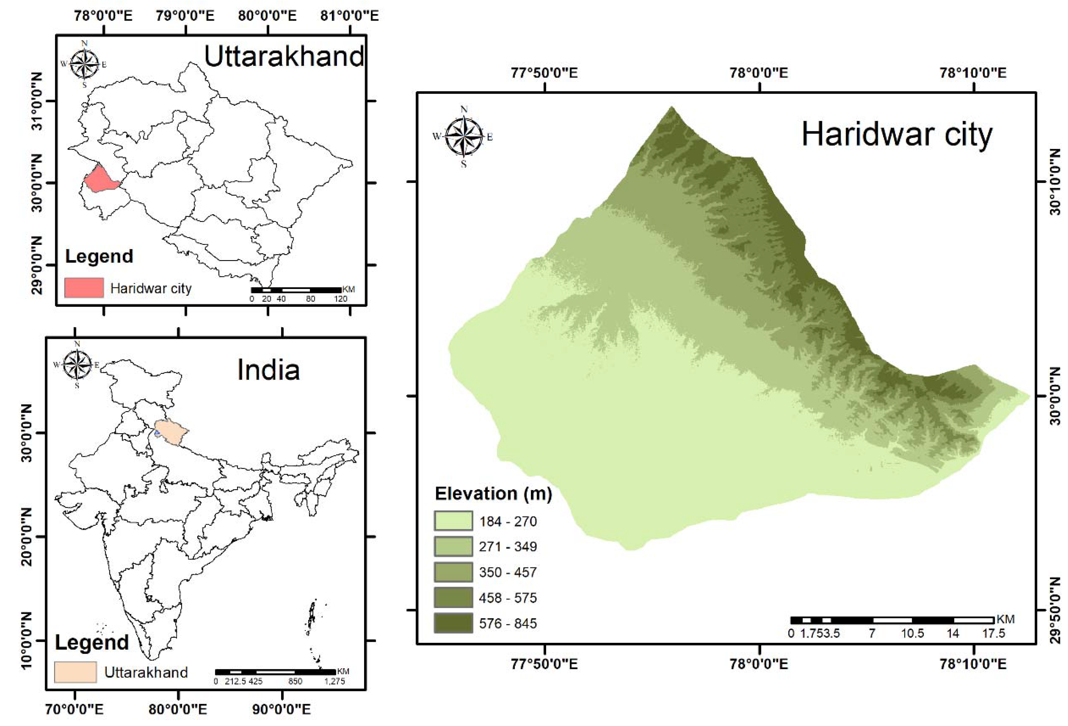
2. Study Area
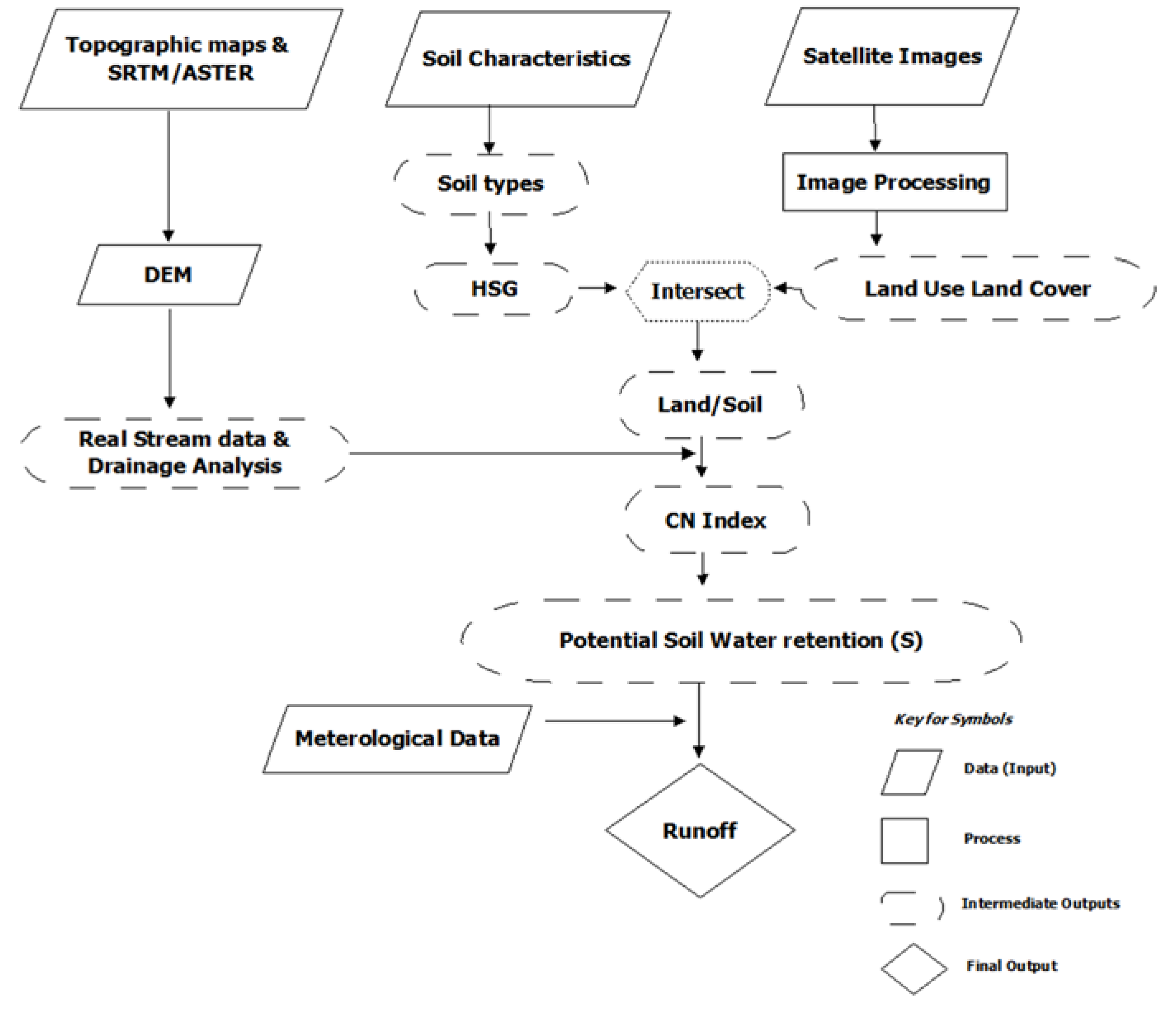
3. Materials and Methods
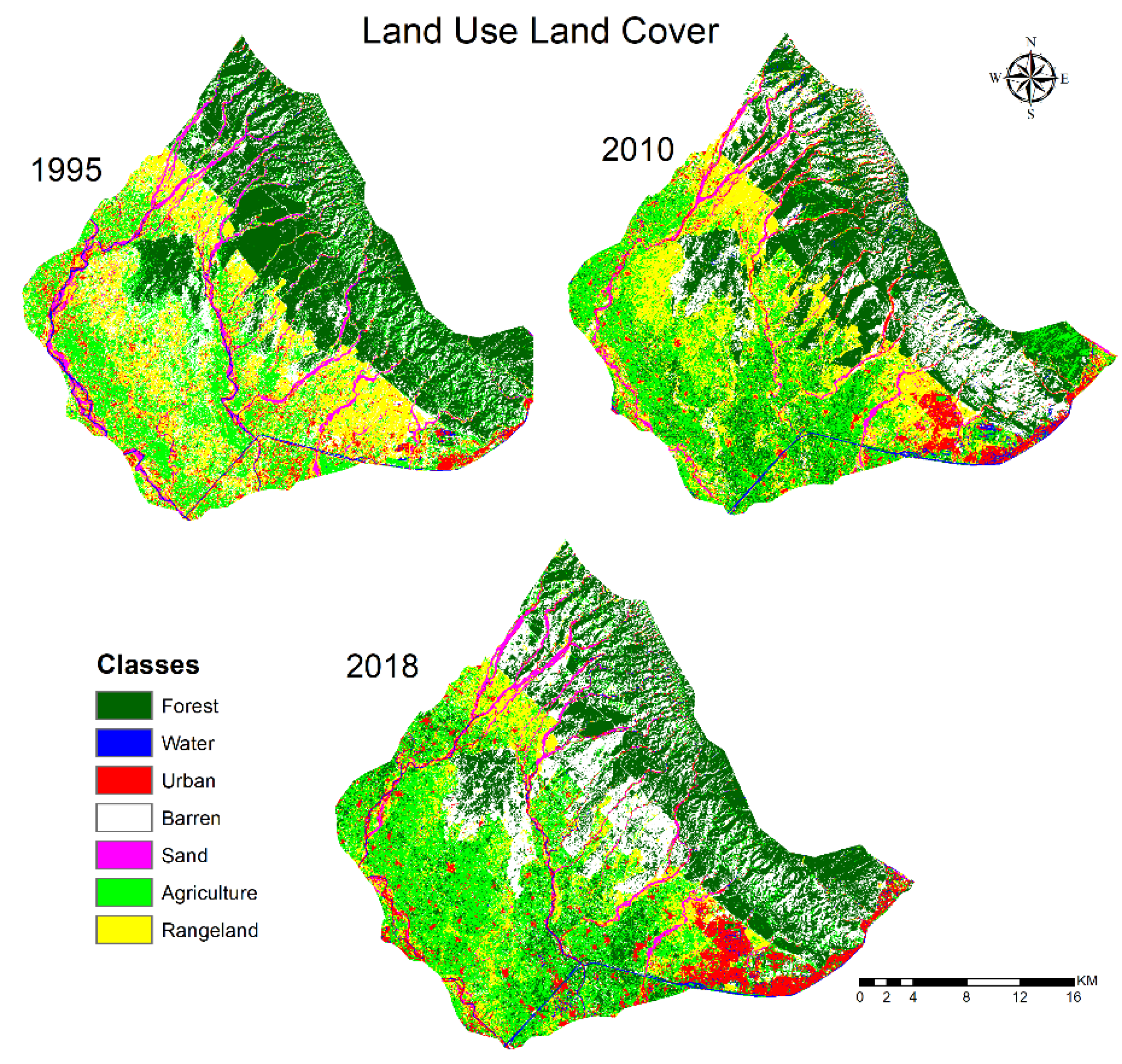
3.1. Land Use Land Cover
3.2. Soil Depth and Texture
3.3. Precipitation and Temperature
3.4. Surface Runoff
3.5. Annual Water Yield
4. Results and Discussion
4.1. Supervised Classification
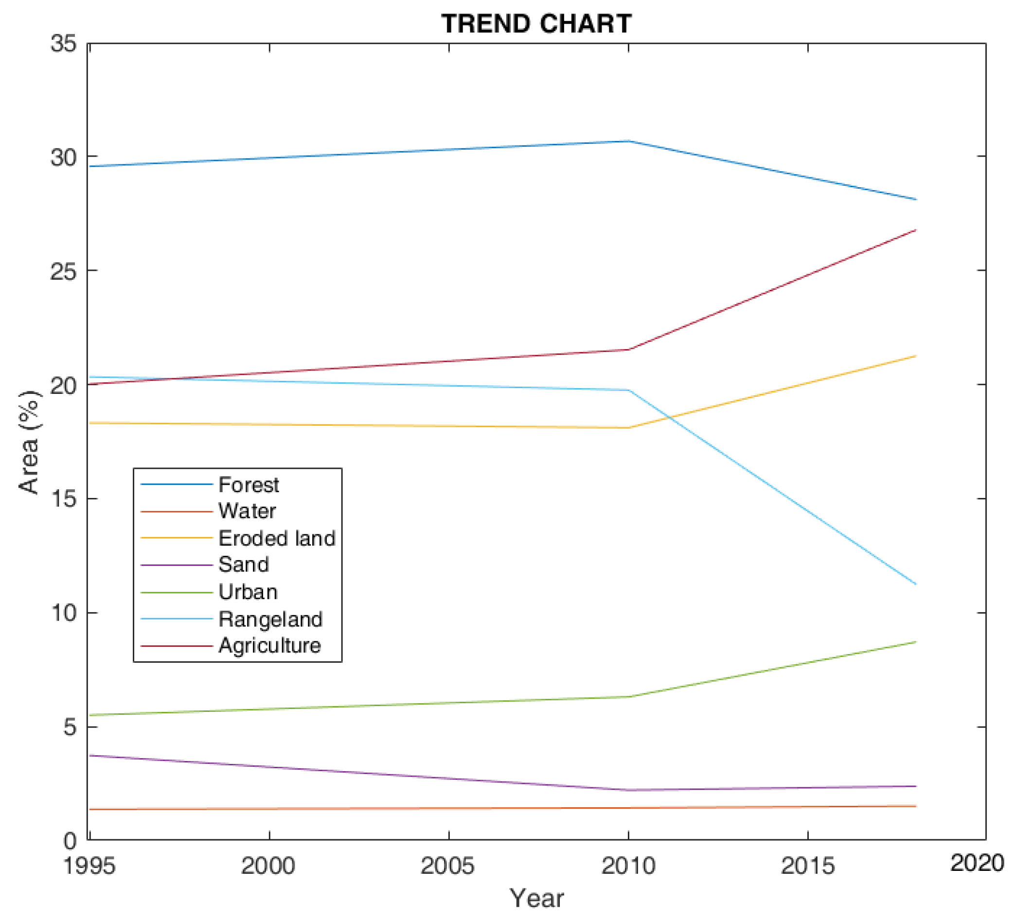
4.2. Trend Analysis of Land Cover Classes
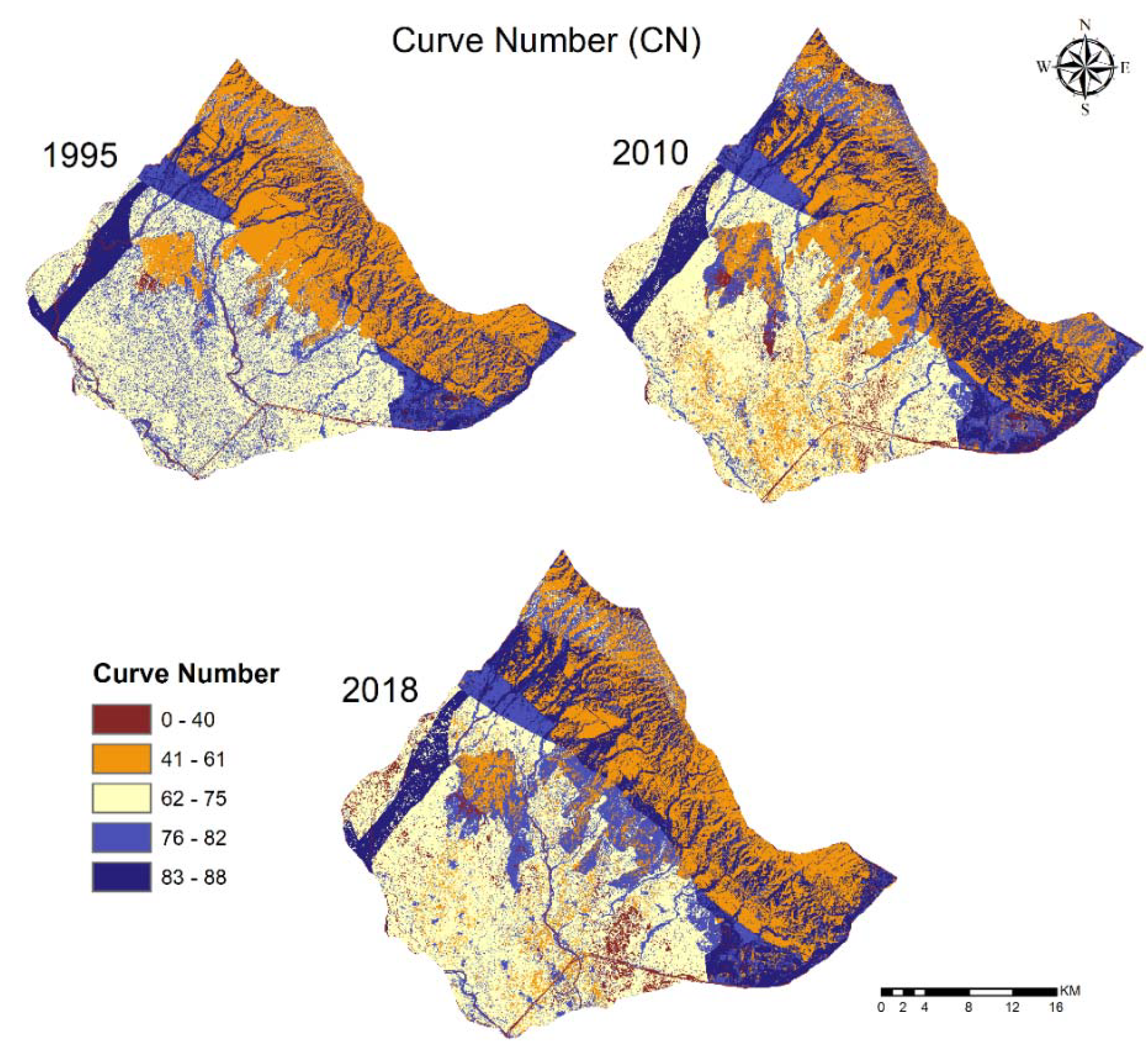
4.3. Curve Number Analysis
4.4. Variation in Area Ratio
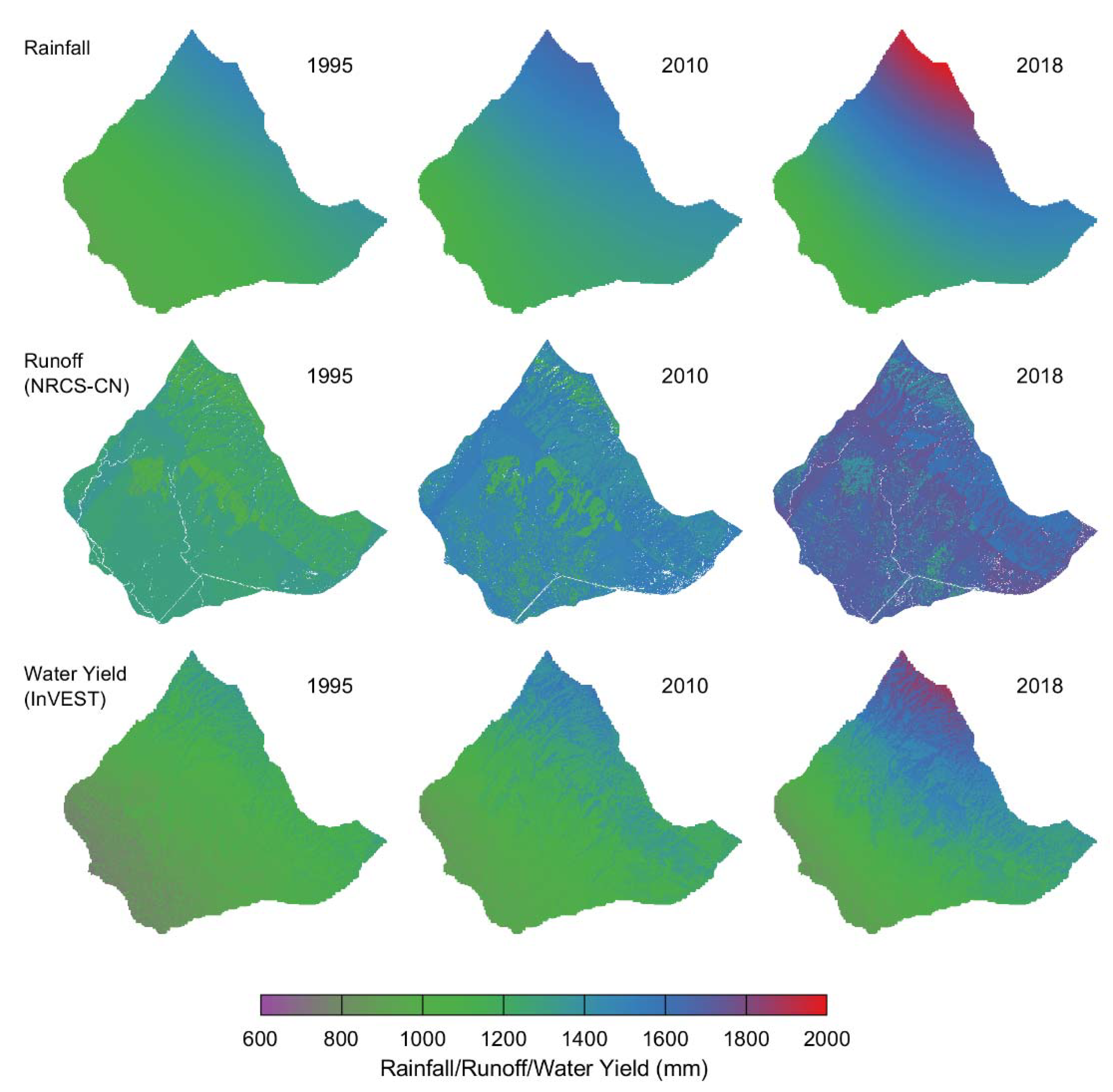
4.5. Runoff Analysis
4.6. Validation Using Alternative Approach
5. Conclusions
Author Contributions
Funding
Acknowledgments
Conflicts of Interest
References
- Anderson, J.R.; Hardy, E.E.; Roach, J.T.; Witmer, R.E. A Land Use and Land Cover Classification System for Use with Remote Sensor Data; U.S. Geological Survey Professional Paper, No. 964; USGS: Washington, DC, USA, 1976.
- Mishra, S.K.; Singh, V.P. Soil Conservation Service Curve Number (SCS-CN) Methodology; Springer: Berlin/Heidelberg, Germany, 2013; Volume 42. [Google Scholar]
- Mishra, S.K.; Sahu, R.K.; Eldho, T.I.; Jain, M.K. An improved IaS relation incorporating antecedent moisture in SCS-CN methodology. Water Resour. Manag. 2006, 20, 643–660. [Google Scholar] [CrossRef]
- Hu, S.; Fan, Y.; Zhang, T. Assessing the effect of land use change on surface runoff in a rapidly urbanized city: A case study of the central area of Beijing. Land 2020, 9, 17. [Google Scholar] [CrossRef] [Green Version]
- Luo, J.; Zhou, X.; Rubinato, M.; Li, G.; Tian, Y.; Zhou, J. Impact of multiple vegetation covers on surface runoff and sediment yield in the small basin of Nverzhai, Hunan province, China. Forests 2020, 11, 329. [Google Scholar] [CrossRef] [Green Version]
- Qi, J.; Lee, S.; Zhang, X.; Yang, Q.; McCarty, G.W.; Moglen, G.E. Effects of surface runoff and infiltration partition methods on hydrological modeling: A comparison of four schemes in two watersheds in the Northeastern US. J. Hydrol. 2020, 581, 124415. [Google Scholar] [CrossRef]
- Shrivastav, M.; Mickelson, S.K.; Webber, D. Using ArcGIS hydrologic modeling and LiDAR digital elevation data to evaluate surface runoff interception performance of riparian vegetative filter strip buffers in central Iowa. J. Soil Water Conserv. 2020, 75, 123–129. [Google Scholar] [CrossRef] [Green Version]
- Xu, C.; Rahman, M.; Haase, D.; Wu, Y.; Su, M.; Pauleit, S. Surface runoff in urban areas: The role of residential cover and urban growth form. J. Clean. Prod. 2020, 262, 121421. [Google Scholar] [CrossRef]
- Steenhuis, T.S.; Winchell, M.; Rossing, J.; Zollweg, J.A.; Walter, M.F. SCS runoff equation revisited for variable-source runoff areas. J. Irrig. Drain. Eng. 1995, 121, 234–238. [Google Scholar] [CrossRef]
- Van Dijk, A.I.J.M. Selection of an appropriately simple storm runoff model. Hydrol. Earth Syst. Sci. 2010, 14, 447. [Google Scholar] [CrossRef] [Green Version]
- Abon, C.C.; David, C.P.C.; Pellejera, N.E.B. Reconstructing the tropical storm Ketsana flood event in Marikina river, Philippines. Hydrol. Earth Syst. Sci. 2011, 15, 1283. [Google Scholar] [CrossRef] [Green Version]
- Soil Conservation Service (SCS). Hydrology, National Engineering Handbook; Soil Conservation Service, USDA: Washington, DC, USA, 1985.
- Shrestha, M.N. Spatially distributed hydrological modeling considering land-use changes using remote sensing and GIS. In Proceedings of the Map Asia Conference, Kuala Lumpur, Malaysia, 13–15 October 2003; pp. 1–8. [Google Scholar]
- Zhan, X.; Huang, M.L. ArcCN-Runoff: An ArcGIS tool for generating curve number and runoff maps. Environ. Model. Softw. 2004, 19, 875–879. [Google Scholar] [CrossRef]
- Mishra, S.K.; Jain, M.K.; Singh, V.P. Evaluation of the SCS-CN-based model incorporating antecedent moisture. Water Resour. Manag. 2004, 18, 567–589. [Google Scholar] [CrossRef]
- Soulis, K.X.; Valiantzas, J.D. SCS-CN parameter determination using rainfall-runoff data in heterogeneous watersheds-the two-CN system approach. Hydrol. Earth Syst. Sci. 2012, 16, 1001. [Google Scholar] [CrossRef] [Green Version]
- Ghate, A.S. Rainfall runoff modeling using SCS-CN method: A GIS based case study of Pawana watershed. J. Water Resour. Eng. Manag. 2019, 3, 50–58. [Google Scholar]
- Pishvaei, M.H.; Sabzevari, T.; Noroozpour, S.; Mohammadpour, R. Effects of hillslope geometry on spatial infiltration using the TOPMODEL and SCS-CN models. Hydrolog. Sci. J. 2020, 65, 212–226. [Google Scholar] [CrossRef]
- Walega, A.; Amatya, D.M.; Caldwell, P.; Marion, D.; Panda, S. Assessment of storm direct runoff and peak flow rates using improved SCS-CN models for selected forested watersheds in the Southeastern United States. J. Hydrol. Reg. Stud. 2020, 27, 100645. [Google Scholar] [CrossRef]
- Hjelmfelt, A.T., Jr. Investigation of curve number procedure. J. Hydraul. Eng. 1991, 117, 725–737. [Google Scholar] [CrossRef]
- Hawkins, R.H. Asymptotic determination of runoff curve numbers from data. J. Irrig. Drain. Eng. 1993, 119, 334–345. [Google Scholar] [CrossRef]
- Grove, M.; Harbor, J.; Engel, B. Composite vs. distributed curve numbers: Effects on estimates of storm runoff depths. J. Am. Water Resour. Assoc. 1998, 34, 1015–1023. [Google Scholar] [CrossRef]
- Moglen, G.E. Effect of orientation of spatially distributed curve numbers in runoff calculations. J. Am. Water Resour. Assoc. 2000, 36, 1391–1400. [Google Scholar] [CrossRef]
- Farran, M.M.; Elfeki, A.M. Evaluation and validity of the antecedent moisture condition (AMC) of Natural Resources Conservation Service-Curve Number (NRCS-CN) procedure in undeveloped arid basins. Arab. J. Geosci. 2020, 13, 275. [Google Scholar] [CrossRef]
- Lian, H.; Yen, H.; Huang, C.; Feng, Q.; Qin, L.; Bashir, M.A.; Wu, S.; Zhu, A.X.; Luo, J.; Di, H.; et al. CN-China: Revised runoff curve number by using rainfall-runoff events data in China. Water Res. 2020, 177, 115767. [Google Scholar] [CrossRef] [PubMed]
- Ormsbee, L.; Hoagland, S.; Peterson, K. Limitations of TR-55 curve numbers for urban development applications: Critical review and potential strategies for moving forward. J. Hydrol. Eng. 2020, 25, 02520001. [Google Scholar] [CrossRef]
- Rao, K.N. Analysis of surface runoff potential in ungauged basin using basin parameters and SCS-CN method. Appl. Water Sci. 2020, 10, 47. [Google Scholar]
- Hassaballah, K.; Mohamed, Y.; Uhlenbrook, S.; Biro, K. Analysis of streamflow response to land use and land cover changes using satellite data and hydrological modelling: Case study of Dinder and Rahad tributaries of the Blue Nile (Ethiopia–Sudan). Hydrol. Earth Syst. Sci. 2017, 21, 5217. [Google Scholar] [CrossRef] [Green Version]
- Pathak, S.; Ojha, C.S.P.; Garg, R.D.; Lakshmi, V. Urbanization and Its Impact on Stormwater Runoff Potential Using Geospatial Tools. In Proceedings of the Geoscience and Remote Sensing Symposium (IGARSS), Valencia, Spain, 22–27 July 2018. [Google Scholar]
- Lal, M.; Mishra, S.K.; Pandey, A.; Pandey, R.P.; Meena, P.K.; Chaudhary, A.; Jha, R.K.; Shreevastava, A.K.; Kumar, Y. Evaluation of the soil conservation service curve number methodology using data from agricultural plots. Hydrogeol. J. 2017, 25, 151–167. [Google Scholar] [CrossRef]
- Bonta, J.V. Determination of watershed curve number using derived distributions. J. Irrig. Drain. Eng. 1997, 123, 28–36. [Google Scholar] [CrossRef]
- Farran, M.M.; Elfeki, A.M. Statistical analysis of NRCS curve number (NRCS-CN) in arid basins based on historical data. Arab. J. Geosci. 2020, 13, 151–167. [Google Scholar]
- Lee, H.K.; Lee, K.H. Impact of representative SCS-CN on simulated rainfall runoff. J. Environ. Sci. Int. 2020, 29, 25–32. [Google Scholar] [CrossRef]
- Shi, W.; Wang, N. An improved SCS-CN method incorporating slope, soil moisture, and storm duration factors for runoff prediction. Water 2020, 12, 1335. [Google Scholar] [CrossRef]
- Xu, A.L. A new curve number calculation approach using GIS technology. In Proceedings of the ESRI 26th International User Conference on Water Resources, San Diego, CA, USA, 7–11 August 2006. [Google Scholar]
- Satheeshkumar, S.; Venkateswaran, S.; Kannan, R. Rainfall–runoff estimation using SCS–CN and GIS approach in the Pappiredipatti watershed of the Vaniyar sub basin, South India. Model. Earth Sys. Environ. 2017, 3, 24. [Google Scholar] [CrossRef]
- Singh, L.K.; Jha, M.K.; Chowdary, V.M. Multi-criteria analysis and GIS modeling for identifying prospective water harvesting and artificial recharge sites for sustainable water supply. J. Clean. Prod. 2017, 142, 1436–1456. [Google Scholar] [CrossRef]
- Ling, L.; Yusop, Z.; Yap, W.S.; Tan, W.L.; Chow, M.F.; Ling, J.L. A calibrated, watershed-specific SCS-CN method: Application to Wangjiaqiao watershed in the three Gorges area, China. Water 2020, 12, 60. [Google Scholar] [CrossRef] [Green Version]
- Rajasekhar, M.; Gadhiraju, S.R.; Kadam, A.; Bhagat, V. Identification of groundwater recharge-based potential rainwater harvesting sites for sustainable development of a semiarid region of southern India using geospatial, AHP, and SCS-CN approach. Arab. J. Geosci. 2020, 13, 24. [Google Scholar] [CrossRef]
- Shi, W.; Wang, N. Improved SMA-based SCS-CN method incorporating storm duration for runoff prediction on the Loess Plateau, China. Hydrol. Res. 2020, 51, 443–455. [Google Scholar] [CrossRef]
- Soulis, K.X.; Valiantzas, J.D.; Dercas, N.; Londra, P.A. Analysis of the runoff generation mechanism for the investigation of the SCS-CN method applicability to a partial area experimental watershed. Hydrol. Earth Syst. Sci. 2009, 13, 605–615. [Google Scholar] [CrossRef] [Green Version]
- Rezaei-Sadr, H. Influence of coarse soils with high hydraulic conductivity on the applicability of the SCS-CN method. Hydrol. Sci. J. 2017, 62, 843–848. [Google Scholar] [CrossRef]
- Al-Juaidi, A.E.M. A simplified GIS-based SCS-CN method for the assessment of land-use change on runoff. Arab. J. Geosci. 2018, 11, 269. [Google Scholar] [CrossRef]
- Arya, S.; Subramani, T.; Karunanidhi, D. Delineation of groundwater potential zones and recommendation of artificial recharge structures for augmentation of groundwater resources in Vattamalaikarai Basin, South India. Environ. Earth Sci. 2020, 79, 102. [Google Scholar] [CrossRef]
- Al-Ghobari, H.; Dewidar, A.; Alataway, A. Estimation of Surface Water Runoff for a Semi-Arid Area Using RS and GIS-Based SCS-CN Method. Water 2020, 12, 1924. [Google Scholar] [CrossRef]
- Karunanidhi, D.; Anand, B.; Subramani, T.; Srinivasamoorthy, K. Rainfall-surface runoff estimation for the Lower Bhavani basin in south India using SCS-CN model and geospatial techniques. Environ. Earth Sci. 2020, 79, 335. [Google Scholar] [CrossRef]
- Nayak, T.R.; Jaiswal, R.K. Rainfall-runoff modelling using satellite data and GIS for Bebas river in Madhya Pradesh. J. Inst. Eng. India 2003, 84, 47–50. [Google Scholar]
- Geena, G.B.; Ballukraya, P.N. Estimation of runoff for Red hills watershed using SCS method and GIS. Indian J. Sci. Technol. 2011, 4, 899–902. [Google Scholar] [CrossRef]
- Gitika, T.; Ranjan, S. Estimation of surface runoff using NRCS curve number procedure in Buriganga Watershed, Assam, India-a geospatial approach. Int. Res. J. Earth Sci. 2014, 2, 1–7. [Google Scholar]
- Ajmal, M.; Kim, T.W. Quantifying excess stormwater using SCS-CN–based rainfall runoff models and different curve number determination methods. J. Irrig. Drain. Eng. 2015, 141, 04014058. [Google Scholar] [CrossRef]
- Jha, M.K.; Chowdary, V.M.; Kulkarni, Y.; Mal, B.C. Rainwater harvesting planning using geospatial techniques and multicriteria decision analysis. Resour. Conserv. Recycl. 2014, 83, 96–111. [Google Scholar] [CrossRef]
- Bhaskar, J.; Suribabu, C.R. Estimation of surface run-off for urban area using integrated remote sensing and GIS approach. Jordan J. Civ. Eng. 2014, 8, 70–80. [Google Scholar] [CrossRef]
- Dinagara Pandi, P.; Saravanan, K.; Mohan, K. Identifying runoff harvesting sites over the Pennar Basin, Andhra pradesh using SCS-CN method. Int. J. Civ. Eng. Technol. 2017, 8, 65–73. [Google Scholar]
- Karunanidhi, D.; Aravinthasamy, P.; Subramani, T.; Roy, P.D.; Srinivasamoorthy, K. Risk of fuoride-rich groundwater on human health: Remediation through managed aquifer recharge in a hard rock terrain, South India. Nat. Resour. Res. 2019, 29, 2369–2395. [Google Scholar] [CrossRef]
- Tallis, H.T.; Ricketts, T.; Nelson, E.; Ennaanay, D.; Wolny, S.; Olwero, N.; Vigerstol, K.; Pennington, D.; Mendoza, G.; Aukema, J.; et al. InVEST 1.004 Beta User’s Guide; The Natural Capital Project: Stanford, CA, USA, 2010. [Google Scholar]
- Shukla, A.K.; Pathak, S.; Pal, L.; Ojha, C.S.P.; Mijic, A.; Garg, R.D. Spatio-temporal assessment of annual water balance models for upper Ganga Basin. Hydrol. Earth Syst. Sci. 2018, 22, 5357–5371. [Google Scholar] [CrossRef] [Green Version]
- Terrado, M.; Acuña, V.; Ennaanay, D.; Tallis, H.; Sabater, S. Impact of climate extremes on hydrological ecosystem services in a heavily humanized Mediterranean basin. Ecol. Indic. 2014, 37, 199–209. [Google Scholar] [CrossRef]
- Hoyer, R.; Chang, H. Assessment of freshwater ecosystem services in the Tualatin and Yamhill basins under climate change and urbanization. Appl. Geogr. 2014, 53, 402–416. [Google Scholar] [CrossRef]
- Thellmann, K.; Blagodatsky, S.; Häuser, I.; Liu, H.; Wang, J.; Asch, F.; Cadisch, G.; Cotter, M. assessing ecosystem services in rubber dominated landscapes in south-east Asia—A challenge for biophysical modeling and transdisciplinary valuation. Forests 2017, 8, 505. [Google Scholar] [CrossRef] [Green Version]
- Pathak, S.; Ojha, C.S.P.; Shukla, A.K.; Garg, R.D. Assessment of Annual Water-Balance Models for Diverse Indian Watersheds. J. Sustain. Water Built Environ. 2019, 5, 04019002. [Google Scholar] [CrossRef]
- Pathak, S.; Ojha, C.S.P.; Zevenbergen, C.; Garg, R.D. Assessing Stormwater Harvesting Potential in Dehradun City Using Geospatial Technology. In Development of Water Resources in India; Springer: Cham, Switzerland, 2017; pp. 47–60. [Google Scholar]
- Pathak, S.; Ojha, C.S.P.; Zevenbergen, C.; Garg, R.D. Ranking of storm water harvesting sites using heuristic and non-heuristic weighing approaches. Water 2017, 9, 710. [Google Scholar] [CrossRef] [Green Version]
- Lee, J.Y.; Kim, N.W.; Kim, T.W.; Jehanzaib, M. Feasible ranges of runoff curve numbers for Korean watersheds based on the interior point optimization algorithm. KSCE J. Civ. Eng. 2019, 23, 5257–5265. [Google Scholar] [CrossRef]
- Jiao, P.; Xu, D.; Li, B.; Yu, Y. A modified Ia-S relationship improves runoff prediction of the USDA-NRCS curve number model. T. ASABE 2019, 62, 771–778. [Google Scholar] [CrossRef]
- Singh, P.; Mishra, S. Determination of curve number and estimation of runoff using Indian experimental rainfall and runoff data. J. Spat. Hydrol. 2019, 13, 1–26. [Google Scholar]
- Zhang, W.Y. Application of NRCS-CN method for estimation of watershed runoff and disaster risk. Geomat. Nat. Hazards Risk 2019, 10, 2220–2238. [Google Scholar] [CrossRef] [Green Version]
- Kastridis, A.; Stathis, D. Evaluation of Hydrological and Hydraulic Models Applied in Typical Mediterranean Ungauged Watersheds Using Post-Flash-Flood Measurements. Hydrology 2020, 7, 12. [Google Scholar] [CrossRef] [Green Version]
- Kastridis, A.; Kirkenidis, C.; Sapountzis, M. An integrated approach of flash flood analysis in ungauged Mediterranean watersheds using post-flood surveys and Unmanned Aerial Vehicles (UAVs). Hydrol. Process. 2020. [Google Scholar] [CrossRef]
- Nastiti, K.D.; An, H.; Kim, Y.; Jung, K. Large-scale rainfall–runoff–inundation modeling for upper Citarum River watershed, Indonesia. Environ. Earth Sci. 2018, 77, 640. [Google Scholar] [CrossRef]
- Pathak, S.; Garg, R.D.; Jato-Espino, D.; Lakshmi, V.; Ojha, C.S.P. Evaluating hotspots for stormwater harvesting through participatory sensing. J. Environ. Manag. 2019, 242, 351–361. [Google Scholar] [CrossRef] [PubMed]
- Pathak, S.; Liu, M.; Jato-Espino, D.; Zevenbergen, C. Social, economic and environmental assessment of urban sub-catchment flood risks using a multi-criteria approach: A case study in Mumbai City, India. J. Hydrol. 2020, 591, 125216. [Google Scholar] [CrossRef]
- Mishra, S.K.; Jain, M.K.; Pandey, R.P.; Singh, V.P. Catchment area-based evaluation of the AMC-dependent SCS-CN-based rainfall–runoff models. Hydrol. Process. 2005, 19, 2701–2718. [Google Scholar] [CrossRef]
- Rahman, H.; Sengupta, D. Preliminary Comparison of Daily Rainfall from Satellites and Indian Gauge Data; CAOS Technical Report, (2007AS1); Indian Institute of Science: Bangalore, India, 2007. [Google Scholar]
- Singh, A.K.; Tripathi, J.N.; Singh, K.K.; Singh, V.; Sateesh, M. Comparison of different satellite-derived rainfall products with IMD gridded data over Indian meteorological subdivisions during Indian Summer Monsoon (ISM) 2016 at weekly temporal resolution. J. Hydrol. 2019, 575, 1371–1379. [Google Scholar] [CrossRef]
- Kumar, T.V.L.; Barbosa, H.A.; Thakur, M.K.; Paredes-Trejo, F. Validation of satellite (TMPA and IMERG) rainfall products with the IMD gridded data sets over monsoon core region of India. In Satellite Information Classification and Interpretation; IntechOpen: Rijeka, Croatia, 2019. [Google Scholar]
- Jena, P.; Garg, S.; Azad, S. Performance Analysis of IMD High-Resolution Gridded Rainfall (0.25°× 0.25°) and Satellite Estimates for Detecting Cloudburst Events over the Northwest Himalayas. J. Hydrometeorol. 2020, 21, 1549–1569. [Google Scholar] [CrossRef]
- Ojha, C.S.P.; Bhunya, P.; Berndtsson, R. Engineering Hydrology, 1st ed.; Oxford University Press: Oxford, UK, 2008; pp. 1–459. [Google Scholar]
- Budyko, M.I.; Ronov, A.B. Evolution of chemical composition of the atmosphere during the Phanerozoic. Geokhimiya 1979, 5, 643–653. [Google Scholar]
- Allen, R.G.; Pereira, L.S.; Raes, D.; Smith, M. Crop Evapotranspiration-Guidelines for Computing Crop Water Requirements-FAO Irrigation and Drainage Paper 56; FAO: Rome, Italy, 1998; Volume 300, p. D05109. [Google Scholar]
- Donohue, R.J.; Roderick, M.L.; McVicar, T.R. Roots, storms and soil pores: Incorporating key ecohydrological processes into Budyko’s hydrological model. J. Hydrol. 2012, 436, 35–50. [Google Scholar] [CrossRef]
- Ward, A.D.; Trimble, S.W. Environmental Hydrology; CRC Press: Boca Raton, FL, USA, 2003. [Google Scholar]
Publisher’s Note: MDPI stays neutral with regard to jurisdictional claims in published maps and institutional affiliations. |


| Class | Percentage (1995) | Percentage (2010) | Percentage (2018) |
|---|---|---|---|
| Forest | 29.57 | 30.68 | 28.12 |
| Water | 1.37 | 1.43 | 1.51 |
| Eroded land | 18.32 | 18.11 | 21.26 |
| Sand | 3.73 | 2.21 | 2.38 |
| Urban | 5.5 | 6.3 | 8.71 |
| Rangeland | 20.34 | 19.76 | 11.23 |
| Agriculture | 20.02 | 21.53 | 26.79 |
| LULC Classes | 1995 | 2010 | 2018 | |||
|---|---|---|---|---|---|---|
| Producer Accuracy (%) | User Accuracy (%) | Producer Accuracy (%) | User Accuracy (%) | Producer Accuracy (%) | User Accuracy (%) | |
| Forest | 74.35 | 82.85 | 76.38 | 83.65 | 77.52 | 83.36 |
| Wasteland | 74.36 | 82.85 | 77.36 | 82.36 | 74.25 | 82.14 |
| Rangeland | 78.94 | 85.71 | 77.69 | 86.32 | 79.69 | 86.31 |
| Agriculture | 79.82 | 85.71 | 81.23 | 86.36 | 79.36 | 85.10 |
| Built up | 84.84 | 80.00 | 85.36 | 78.36 | 84.69 | 81.23 |
| Sand | 72.97 | 77.84 | 73.25 | 79.32 | 73.36 | 79.25 |
| Water | 84.00 | 60.00 | 85.36 | 72.00 | 85.00 | 65.00 |
© 2020 by the authors. Licensee MDPI, Basel, Switzerland. This article is an open access article distributed under the terms and conditions of the Creative Commons Attribution (CC BY) license (http://creativecommons.org/licenses/by/4.0/).
Share and Cite
Pathak, S.; Ojha, C.S.P.; Garg, R.D.; Liu, M.; Jato-Espino, D.; Singh, R.P. Spatiotemporal Analysis of Water Resources in the Haridwar Region of Uttarakhand, India. Sustainability 2020, 12, 8449. https://0-doi-org.brum.beds.ac.uk/10.3390/su12208449
Pathak S, Ojha CSP, Garg RD, Liu M, Jato-Espino D, Singh RP. Spatiotemporal Analysis of Water Resources in the Haridwar Region of Uttarakhand, India. Sustainability. 2020; 12(20):8449. https://0-doi-org.brum.beds.ac.uk/10.3390/su12208449
Chicago/Turabian StylePathak, Shray, Chandra Shekhar Prasad Ojha, Rahul Dev Garg, Min Liu, Daniel Jato-Espino, and Rajendra Prasad Singh. 2020. "Spatiotemporal Analysis of Water Resources in the Haridwar Region of Uttarakhand, India" Sustainability 12, no. 20: 8449. https://0-doi-org.brum.beds.ac.uk/10.3390/su12208449