Route and Path Choices of Freight Vehicles: A Case Study with Floating Car Data

Abstract

According to the literature, the path choice decision process of a user of a (road) transport network, named path choice problem (PCP), is composed of two levels/models: the definition of perceived alternative paths (choice set) and the choice of one path in the path choice set. The path choice probability can be estimated with two models: a choice model of the path choice set and a choice model of a path (Mansky paradigm). In this research, the paper’s contribution concerns two elements: extension of the PCP paradigm (two-level models) consolidated in the literature to the route choice decision process (vehicle routing problem (VRP)) and identification of common elements in the PCP and VRP concerning the criteria in the two decision levels and the procedure for route and path selection and choice. The experiment concerns the comparison of observed routes with simulated and optimized routes of commercial vehicles to analyse the level of similarity and coverage. The observed routes are extracted from floating car data (FCD) from commercial vehicles travelling inside a study area inside the Calabria Region (Southern Italy). The comparison is executed in terms of similarity of the sequences of nodes visited between observed routes and simulated/optimized routes.

1. Introduction

The general objective of the research is the modelling of a path and route choice of commercial vehicles travelling on a road network to distribute freight to several destinations (clients) in a suburban area. According to the authors:

• a path is a sequence of loopless and consecutive links (of a network) connecting two nodes without planned stops between the two nodes (i.e., in freight distribution, intermediate pickup and delivery points);
• a route is a sequence of consecutive paths connecting an initial node and a final node, which could also be the same (closed route) (i.e., in freight distribution, the initial and final nodes could be depots; the origins and destinations are intermediate pickup and delivery points).

In the literature, the path choice decision process of an individual user of a (road) transport network could be composed of two levels:

(a)

the definition of perceived alternative paths (included in a path choice set);

(b)

the choice of one path in the path choice set.

The choice probability of a path can be estimated with two models:

(a)

a choice model of the path choice set;

(b)

a choice model of a path, given the path choice set.

The choice probability of a path, considering the two choice models, (a) and (b), could be estimated according to the Mansky paradigm [1]. Paths belonging to the path choice set can be generated with a monocriterion or multicriterion approach. Some users could consider the monocriterion approach, generating the paths with the same criterion; other users could consider the multicriterion approach, generating one or more paths for each criterion considered. By adopting more than one criterion, the same path could be generated with different criteria. Generally, a set of criteria (i.e., minimum travel time, travel distance, travel cost, energy consumption) is considered, and one or more paths for each criterion are generated.

In the existing literature, the route choice is evaluated as an optimum sequence of visited nodes inside a vehicle routing problem.

In this research, the paper’s contribution concerns the experimental analysis and comparison of a set of criteria for both the path and route choice decision processes. Data supporting the analysis concern sequences of stops to serve clients and paths between two consecutive stops of freight vehicles. The sources of data are GPS positions of a sample of freight vehicles, so-called floating car data (FCD), travelling along a road network inside a study area in the Calabria Region (Italy).

The experiment presented in the paper concerns a comparison of observed routes and simulated and optimized routes of freight vehicles in terms of level of similarity and coverage according to each of three criteria: minimum travel time, minimum travel distance, and minimum energy consumption.

The remaining part of the paper is structured as follows. Section 2 reports the consolidated methods regarding data for freight demand models and the route/path choice decision process. Section 3 shows empirical evidence of routes of commercial vehicles travelling in a suburban area extracted from commercial FCD. Section 4 reports the conclusions and the research perspectives.

2. Consolidated Methods

This section reports the consolidated methods regarding data for freight demand modelling, in particular data for vehicle-based freight flow models (Section 2.1); route and path choice in terms of decisions, procedures, and performances (Section 2.2). Section 2.3 is presented as the research contribution.

Figure 1 reports a flowchart of the methodological components analysed in the research: models (described inside the ellipses) and input and output data (described inside the boxes). Each component is presented in detail in a section of the paper according to the sequence of their appearance in the flowchart.

2.1. Data

Freight demand models may be classified according to two types of flow representation [2,3,4]:

• commodity-based models, which represent freight flows from one (or more) production area(s) to one (or more) consumption area(s);
• vehicle-based models, which represent both logistic flows (i.e., shipment size, frequency of restocking, structure of the supply chain) or transport flows (i.e., mode services, routes).

The specification–calibration–validation process of freight demand models requires data that have a different nature according to the above classification.

Commodity-based models require data on production–consumption freight flows, traditionally collected by means of articulated financial or quantity flow surveys. They are suitable for aggregate estimates, but they do not allow for providing logistic and transport elements.

Vehicle-based models for logistic flows require data on relationships and dependencies among producers, logistic operators, carriers, and multimodal transport operators. They are collected by means of costly and low-responsive surveys, given the competitive attitude of the different actors in the supply chain. The aim is to provide insights into the structure of the supply chain, composed of nodes, such as warehouses, echelons, transport stops, and links, as different mode-service paths and routes [4].

Vehicle-based models for transport flows require data on the trips of freight vehicles in terms of stops from the depot to the clients and paths between two consecutive stops on the (road) transport network. Data are generally collected by means of surveys, such as travel diary surveys and traffic counts data on multimodal transport operators, logistic operators, and carriers. Recently, data from vehicles’ GPS positions (FCD) are used to build time–space freight vehicle trajectories along the network.

The paper focuses on data that would be able to support the building process of vehicle-based models for transport flows, with a specific focus on path and route choice models. Data provide sequences of stops from the depot to the clients and paths between two consecutive stops of freight vehicles travelling in a suburban area.

Data are extracted from GPS positions of a sample of freight vehicles (FCD) travelling along a road network inside a study area in the Calabria Region (Italy). Several papers available in the literature deal with the contribution of GPS technology in the characterization of goods movements (see, among others, [5,6] for the urban case and [7] for the national case) and, in general, in the estimation and diagnosis of traffic conditions [8,9].

2.2. Route and Path Choice

Decision and Procedure

Route and path choices are two decision levels associated with operators and drivers in the freight distribution process. At the route level, the order of visits of freight pickup and delivery points has to be defined. At the path level, the sequence of links connecting two successive pickup and delivery points has to be defined.

The decisions are assumed by the operator, or by the driver, based on procedures derived from simulation, optimization, and experience.

The decisions in the two levels could be assumed with identical or different procedures (i.e., at the route level by means of an optimization procedure and at the path level based on experience). In this work, the two decision levels of a sample of independent users are observed and analysed. The choices are generated with consolidated simulation and optimization and then compared with the observed ones in order to identify common elements in the two decision levels and among different users.

Performances

In urban and suburban areas, freight vehicles share road infrastructures with passenger vehicles. Generally, the percentage of freight vehicles is low compared with that of passenger vehicles. For instance, in Italy, with respect to the total registered vehicles at the national level in 2019 [10], the percentage of freight vehicles was 9.6%. In addition, the sample analysed was low compared with all the freight vehicles circulating in the examined area. For this reason, it can be assumed that travel performances (i.e., travel time, congestion) are determined by passenger and freight mobility, but they are constant (rigid) with respect to route and path changes of the analysed freight vehicles.

For this reason, it is assumed that the travel performances on the road transport system change in space and time. Travel performances are obtained from data derived from (i) a monitoring system model and (ii) a transport system model to simulate passenger mobility and freight mobility that use reverse assignment procedures [11]. Travel time is an input of the procedure.

(i)

As far as the monitoring system is concerned, a reliable system for the purpose of this analysis is connected to the use of anonymous FCD, travelling in the study area, and related to passenger and freight vehicles and not only belonging to the sample analysed (for details, see [12]).

(ii)

As far as the transport system models are concerned, the following models are used: network models for the supply subsystem, by calibrating the link cost functions [13] using data derived from FCD; behavioural models for the travel demand subsystem, by calibrating the travel demand functions from traffic counts; and static or dynamic models for the interaction between supply and travel demand (for details, see [14]).

2.2.1. Route

According to the scientific literature, the best route is the output of a vehicle routing problem (VRP). The route r is obtained from the solution of an optimization problem (minimum), where an objective function (φ) is minimized:

Minimum φ(r)

The objective function is evaluated with a monocriterion approach, and it evaluates the operator cost to travel along the route. In the objective function, one of the following costs, or a weighted sum of them, is generally considered: travel time, travel cost, management cost, energy consumptions, etc.

The solution problem is subject to a set of constraints. The most common constraints are time windows for freight collection and delivery, maximum cost, maximum time, maximum number and type of vehicle, load capacity, energy autonomy, environmental thresholds, etc.

The solution procedures are heuristic for a real-time solution of a real-size problem (for details, see as examples [15,16,17,18]).

2.2.2. Path

In the scientific literature, the best path is the output of a path choice problem (PCP). The path p is obtained from the solution of a simulation problem with two levels and sequential models ([19,20,21,22]):

• generation of the choice set perceived by the users;
• choice of the path belonging to the perceived choice set.

The generation of the choice set I perceived by the users is obtained with a multicriterion procedure. For each criterion, one or more perceived paths are generated. The most common criteria adopted in the literature are minimum travel time, minimum monetary cost, minimum congestion, minimum energy consumption, maximum motorway, etc.

The choice of the path belonging to the choice set is simulated with behavioural models (i.e., logit, C-logit, probit), where it is assumed that the user chooses the path p of maximum utility, U_p, assumed to be a random variable (monocriterion). For this reason, the path choice probability, prob_p, associated with each path p is evaluated as:

prob_p = Probability(U_p > U_p’;∀ p, p’∈ I; p’≠ p)

The problem is solved with mixed monocriterion and multicriterion approaches. The route choice model is the core of the static and dynamic assignment models [14,15,16,17,18,19,20,21,22,23].

2.3. Research Contribution

The VRP and the PCP are generally studied with different approaches in the literature. As reported in Section 2.2, the two problems are different according to:

• the objective function (monocriterion vs. monocriterion and multicriteria);
• decision procedure (optimization vs. simulation).

The VRP and the PCP are two sequential decision levels adopted by the same decision maker. The thesis of this research presented in the paper is that a similar behaviour is adopted in the two problems.

In order to demonstrate the above thesis, a sample of users is observed and analysed to identify common elements in the decision process concerning

• the criteria adopted in the two decision levels;
• the procedure adopted for route and path selection and choice.

3. Experimental Case Study

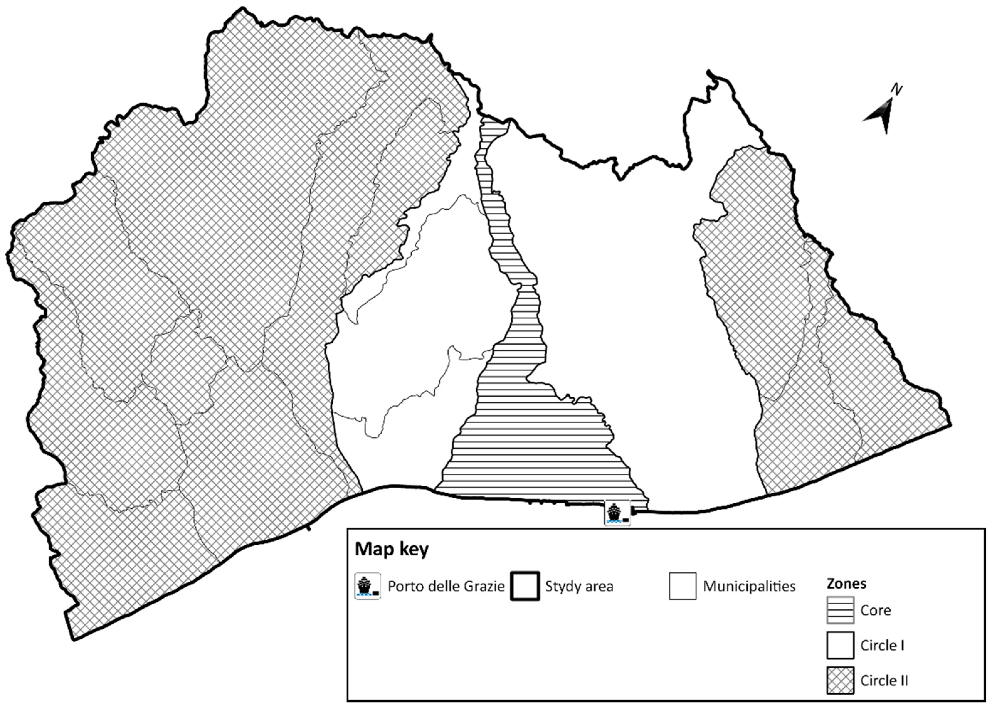
The experiment took place in a study area, including several municipalities located in a section of the province of Reggio Calabria along the Ionian coast in Southern Italy (see Figure 2).

3.1. Data

The available experimental data, extracted from commercial FCD, concern routes of commercial vehicles travelling inside the study area. The available FCD dataset has been used to obtain trips of commercial vehicles. The number of monitored vehicles (944) is about 2% (penetration rate) of the vehicles travelling inside the province of Reggio Calabria. In the province, with respect to the total registered vehicles at the provincial level in 2019 [10], the percentage of freight vehicles was 11.5%.

The available commercial FCD cannot be used directly to analyse routes and paths. It is necessary to process rough FCD by applying a sequence of temporal and spatial filtering criteria in order to obtain a set of observed routes of commercial vehicles.

Regarding temporal criteria, the first temporal selection concerns the period of the year. The available FCD dataset spans 2 summer weeks and contains 289,489 spatial–temporal vehicle positions, grouped in elementary trips and defined as a succession of consecutive spatial positions of the same vehicle from the time instant in which the movement begins (start) to the time instant in which the movement stops (stop).

The observed data refer to a period before the COVID-19 lockdown. Whether the freight distribution behaviour according to the criteria adopted (that is one of the points analysed in this paper) changes or not in relation to the lockdown period will be investigated in further studies.

By applying the above filtering criterion, the number of elementary trips that cross the province of Reggio Calabria was 14,278, operated by 412 monitored vehicles and counted only once (

Table 1. Estimation of generated trips of commercial vehicles (trips/day).

Week	Total Points	Commercial Vehicles	Elementary Trips	Path
1	148,643	461	7938	6242
2	140,846	483	6340	5047
Total	289,489	412 *	14,278	11,289

* Counted only once.

).

The second temporal selection criterion is finalized to identify the paths of each vehicle as defined in Section 1. Paths of a single vehicle are obtained from elementary trips. Two successive elementary trips (that is, when the last spatial position of the first trip and the initial one of the second trip are coincident) belong to the same path according to the first (lower) temporal threshold (limit LAG1).

The temporal spacing is measured as the difference between the “start” instant of the second trip and the “stop” instant of the first one. According to a previous work [12], the value of the limit LAG1 is assumed to be equal to 5 min. By applying this selection criterion, the number of paths is 11,289.

The third temporal selection criterion aims to identify the freight pickup and delivery points. In this case, two consecutive paths are compared, with the destination point of the first path coincident with the origin point of the second one. Two consecutive paths belong to the same route, as defined in Section 1, if the time spacing is lower than a threshold value. In order to obtain this threshold value, the frequencies of temporal gaps have been plotted (Figure 3). The results of the frequency analysis lead to the identification of an upper limit LAG2, which separates the individual paths of commercial vehicles from the paths composing a route. The value of limit LAG2 is equal to 20 min in this case.

Furthermore, the Limit LAG1 value allows the classification of the trajectories: isolated trips (path) and trip chains (route).

Based on spatial criteria, from total points and the relative trajectories registered in relation to vehicle movements, trajectories are classified into:

• external trajectories, selecting vehicle movements that have no point in the study area;
• study area trajectories, which have at least one point inside the study area.
• By considering study area trajectories, it is possible to identify:
• internal trajectories with both origin and destinations inside the study area (I/I);
• outcoming trajectories with origin inside the study area and destinations outside the study area (I/E);
• incoming trajectories with origin outside the study area and destinations inside the study area (E/I);
• crossing trajectories with origin and destinations outside the study area but with at least one point inside the area (E-E).

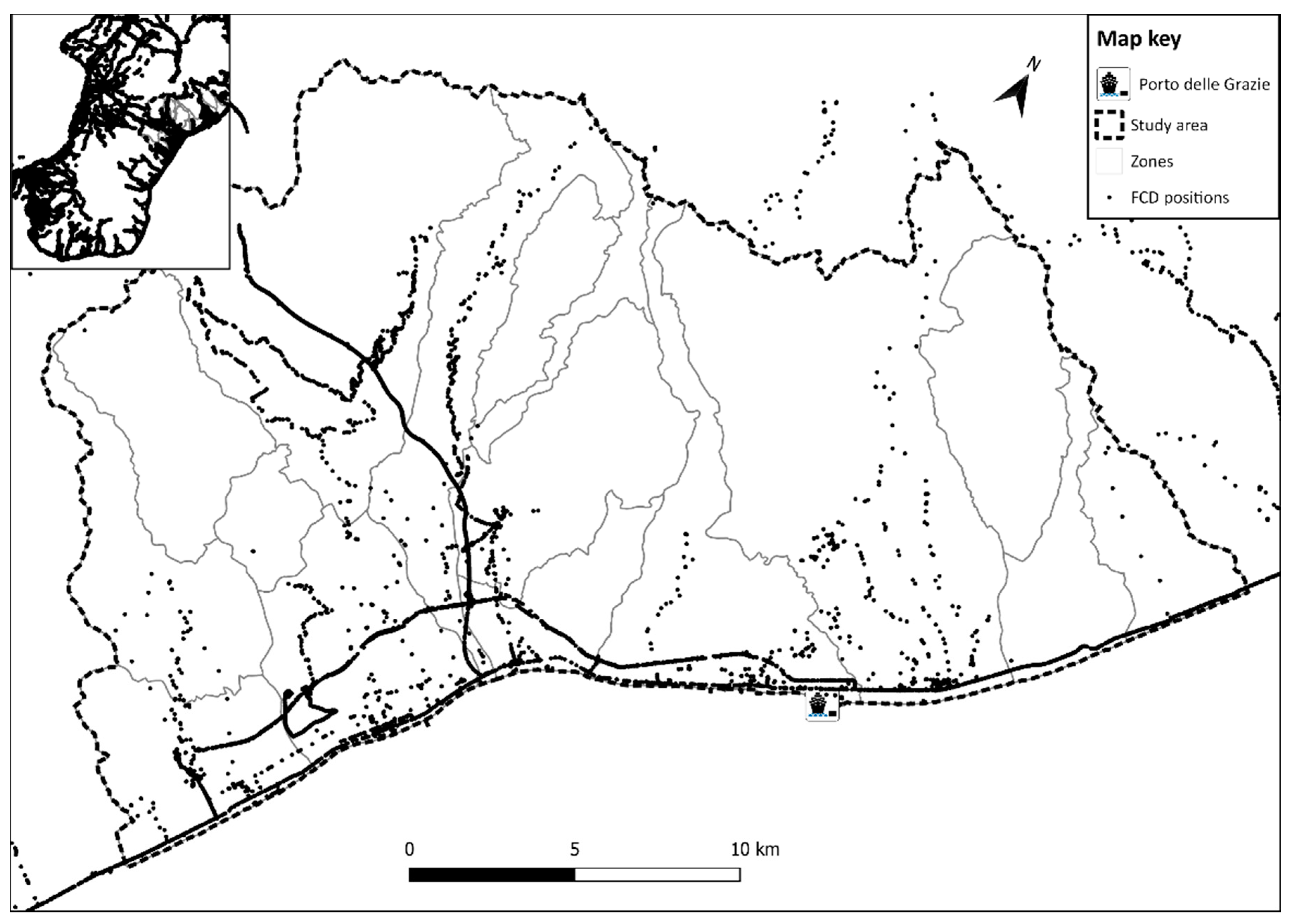
In the study case, 11,289 paths were identified (Figure 4) starting from the original 289,489 total points related to 412 vehicles.

By applying spatial filtering, the total paths (11,289) are divided into 10,574 external paths without any point in the study area and 715 study area paths with at least one point in the study area. By selecting study area paths, there are 523 internal paths (I/I), 73 outcoming paths (E/I), 73 incoming paths (I/E), and 46 crossing paths. These numbers are specified for 2 selected summer weeks in

Table 2. Classification of paths.

Week	Paths with Respect to the Study Area				Origin/Destination of the Internal Paths with Respect to the Study Area *
	All	External	Internal	I/I	I/E	E/I	E/E	Internal
1	6242	5887	362	269	37	38	18	362
2	5047	4687	353	254	36	35	28	353
Total	11,289	10,574	715	523	73	73	46	715

* I = internal to the study area, E = external to the study area.

.

The total number of paths in the 2 summer weeks (715) was operated by 61 commercial vehicles, corresponding to approximately 6% of the total number of monitored commercial vehicles. By assuming limit LAG2 as threshold, the total number of routes analysed was equal to 407, which included 258 isolated paths and 149 routes.

Table 3. Synopsis of observed vehicles, paths, and routes.

	Path	Route	Vehicle
Isolated	258 (36.1%)	258 (63.4%)	52
Chained	457 (63.9%)	149 (36.6%)	34
Total	715 (100%)	407 (100%)	--

reports a synopsis of observed vehicles, paths, and routes.

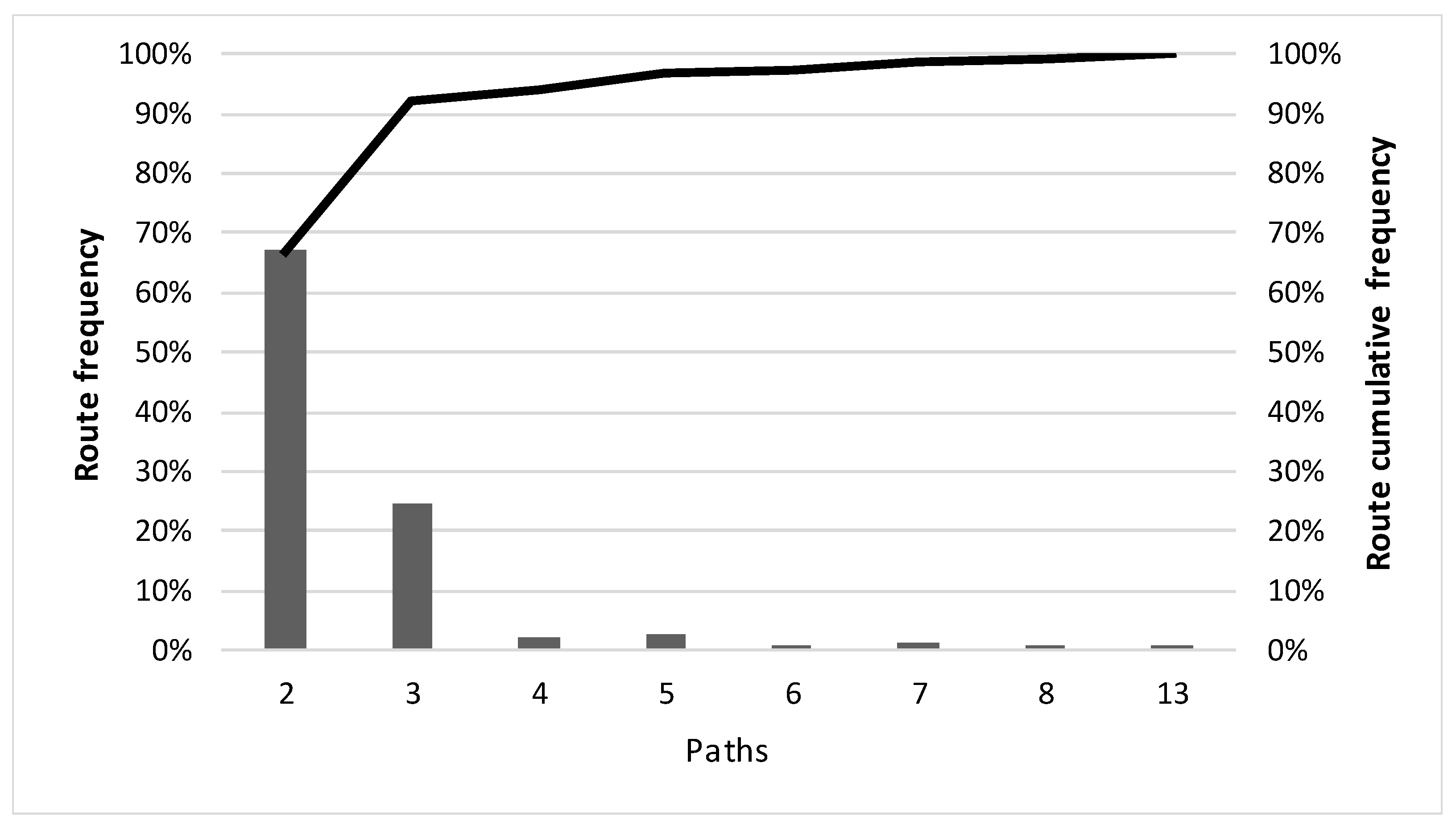
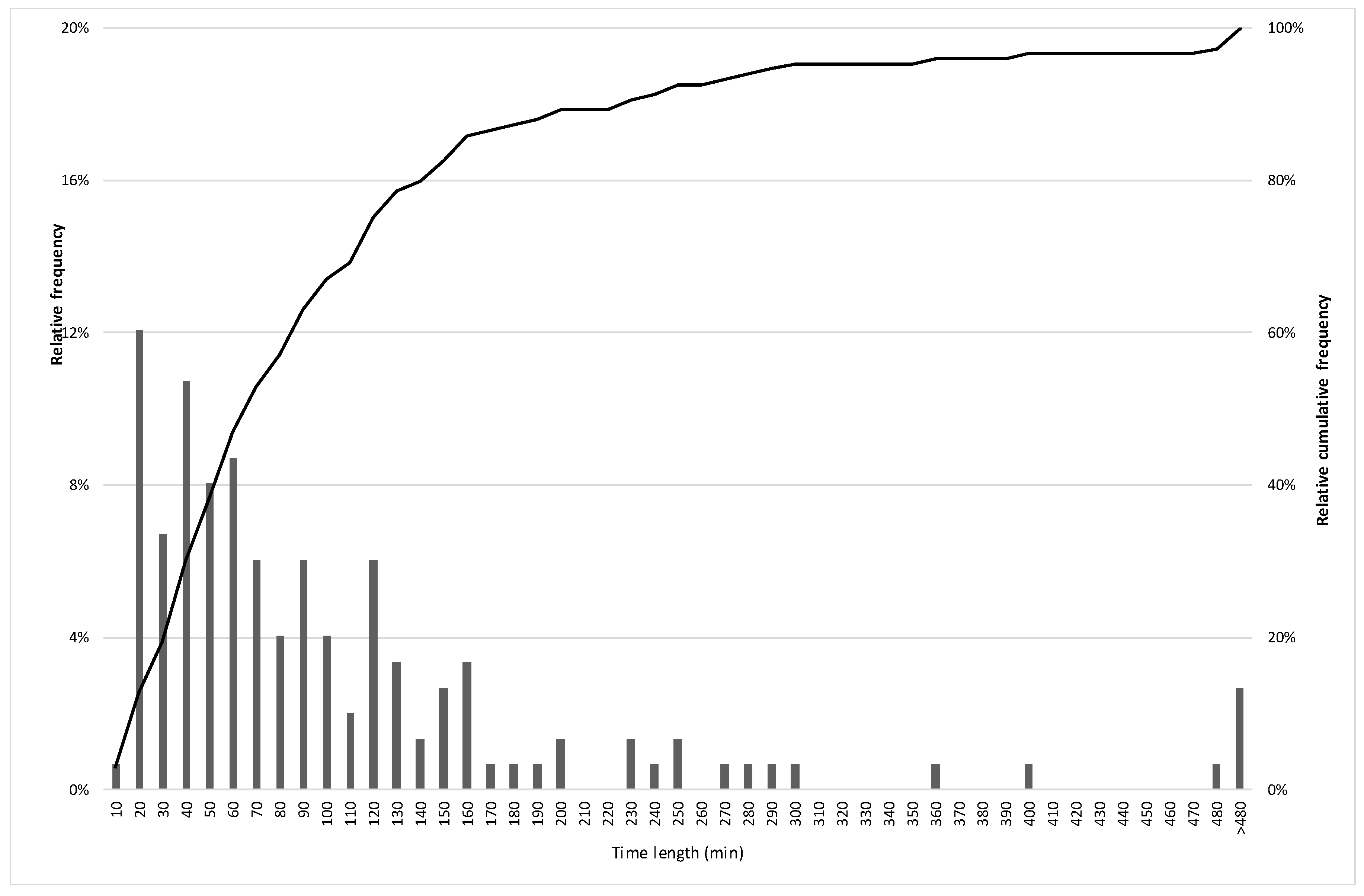
By examining the set of routes, a frequency analysis (Figure 5) was carried out in order to identify the percentage distribution of the number of composing paths. It is worth noting that 137 routes (92% of the total routes) were made up by fewer than three paths. The remaining routes (12 routes, 8% of the total) were the object of the analysis presented in this paper, as they represented the freight pickup and delivery process. The selected routes included 73 paths, with an average total time of a route less than 70 min in 73% of the cases (Figure 6).

3.2. Route and Path Choice

The results were obtained by means of a network model (graph and calibrated link cost functions) by estimating the performances of the road transport infrastructures in the study area.

The comparison was executed in terms of:

• similarity of the sequences of nodes visited between observed routes and simulated/optimized routes: number and percentages of pairs related to four criteria: minimum travel time, travel distance, travel cost, and energy consumption;
• similarity of the paths composing the routes between observed routes and optimized routes: number and percentage of paths related to the four criteria;
• coverage of the criteria of the observed routes and paths.

3.2.1. Route Choice

Table 4. Comparisons of the observed (FCD) simulated and optimized routes.

ID	Paths	FCD		Simulated Route			Optimized Route
		Travel Time	Time Stop	Chosen Route			Time Criterion			Distance Criterion			Energy Criterion
		[min]	[min]	[min]	[km]	[kWh]	[min]	[km]	[kWh]	[min]	[km]	[kWh]	[min]	[km]	[kWh]
61	13	121	104	115	77	16.6	93	69	8.92	100	67	9.01	100	67	9.01
40	8	129	96	116	106	21.3	108	107	14.82	111	106	15.03	111	106	15.03
81	7	115	37	114	93	21.0	95	79	10.53	95	79	10.53	95	79	10.53
56	7	48	41	46	30	6.4	40	30	4.38	41	30	4.34	41	30	4.34
112	6	100	134	84	72	14.6	38	29	5.55	38	29	5.54	38	29	5.54
79	5	58	20	57	45	11.7	41	31	7.24	41	31	7.24	41	31	7.24
48	5	80	55	71	49	10.0	40	35	4.69	40	35	4.69	40	34	4.96
54	5	56	46	54	53	12.6	51	52	10.79	69	49	10.78	58	62	8.62
55	5	54	28	42	31	3.8	36	31	0.81	40	30	0.75	40	30	0.75
77	4	26	49	24	17	3.7	22	16	1.26	22	16	1.26	22	16	1.26
74	4	37	24	37	21	5.9	33	21	4.34	33	21	4.34	33	21	4.34
85	4	55	21	43	38	7.6	38	39	5.21	43	33	4.90	42	33	4.89
Average	6.1	73.3	54.6	67.3	52.7	8.0	52.8	44.9	6.5	55.9	43.8	6.5	55.1	44.8	6.4
Total	73	879	655	807	632	95.9	634	539	79	671	526	78	661	538	77

reports the main characteristics of the sample of routes obtained from the elaboration of the FCD. An ID code identifies each route. The characteristics are the number of paths composing each route, the time spent at the stop, and the total travel times. The sample comprehended 12 routes and 73 paths, 6.1 paths on average; the average time spent at the stops was 55 min; and the average travel time was 73 min.

The same table reports a comparison of the observed (FCD) simulated and optimised routes. The following information is reported for each route:

• time, distance, and energy attributes of chosen routes estimated by means of transport system models (network model);
• time, distance, and energy attributes of optimized routes adopting each selected criterion (time, distance, and energy of best routes).

Figure 7 reports a graphical representation of three routes of the sample (IDs 40, 56, and 81). Each route is represented in terms of origin point, sequence of travelled road infrastructure, intermediate stops, and final destination point.

From available information, two analyses of similarity of observed and optimized routes were performed. The first analysis compared the order of the visited nodes by considering the number of connected pairs (

Table 5. Similarity of the order of visited nodes between the observed route and the best route: number of pairs.

ID	Number of Paths	Similarity of the Order of Visited Nodes between the Observed Route and the Best Route
		Same Direction						Opposite Direction						Both Directions
		Time		Distance		Energy		Time		Distance		Energy		All Criteria
61	13	4	31%	3	23%	3	23%	3	23%	4	31%	5	38%		9	69%
40	8	8	100%	1	13%	1	13%	0	0%	5	63%	5	63%		8	100%
81	7	2	29%	2	29%	2	29%	4	57%	2	29%	2	29%		6	86%
56	7	5	71%	5	71%	5	71%	1	14%	1	14%	1	14%		6	86%
112	6	2	33%	2	33%	2	33%	0	0%	0	0%	0	0%		2	33%
79	5	5	100%	5	100%	5	100%	0	0%	0	0%	0	0%		5	100%
48	5	2	40%	2	40%	2	40%	0	0%	0	0%	0	0%		2	40%
54	5	2	40%	3	60%	3	60%	1	20%	0	0%	0	0%		3	60%
55	5	2	40%	2	40%	2	40%	1	20%	1	20%	1	20%		3	60%
77	4	2	50%	2	50%	0	0%	0	0%	0	0%	0	0%		1	25%
74	4	1	25%	1	25%	1	25%	0	0%	0	0%	0	0%		3	75%
85	4	4	100%	4	100%	4	100%	0	0%	0	0%	0	0%		4	100%
Mean	6.1	3.3	54%	2.7	44%	2.5	41%	0.8	13%	1.1	18%	1.2	20%		4.3	70%
All	73	39	53%	32	44%	30	41%	10	14%	13	18%	14	19%		52	71%

). The second analysis compared the order of the visited nodes by considering the percentage with respect to the considered criteria (Table 5). Both analyses took into account the route direction, which could be the same when the order of visit was the same or the opposite when the order of visit was inverted. The same analysis was performed by not considering the direction (all directions). These differentiations were considered in order to verify whether direction can influence the choices’ criterion.

Some evidence emerges from the analysis of the experimental results.

From the results of the first analysis (

Table 6. Similarity of the order of visited nodes between the observed route and the best route: percentage for each criterion.

ID	Number of Paths	Similarity of the Order of Visited Nodes between the Observed Route and the Best Route
		Same Direction			Opposite Direction			Both Directions
		Time	Distance	Energy	Time	Distance	Energy	All Criteria *
61	13	14%	18%	3%	9%	9%	14%	24%
40	8	100%	8%	8%	0%	73%	77%	100%
81	7	8%	21%	11%	73%	13%	19%	81%
56	7	57%	53%	50%	15%	17%	17%	72%
112	6	23%	23%	28%	0%	0%	0%	23%
79	5	100%	100%	100%	0%	0%	0%	100%
48	5	38%	34%	27%	0%	0%	0%	38%
54	5	17%	14%	79%	5%	0%	0%	22%
55	5	14%	10%	8%	4%	1%	1%	18%
77	4	49%	50%	0%	0%	0%	0%	49%
74	4	59%	59%	74%	12%	13%	4%	71%
85	4	100%	100%	100%	0%	0%	0%	100%
Mean	6.1	48%	41%	40%	10%	11%	11%	58%
All	73	48%	31%	35%	9%	17%	8%	57%

* The time is considered for the percentage evaluation of all criteria.

) emerged that no criterion prevailed over the others. The “time” criterion prevailed over the others only in route 40. The observed route had the same characteristics as the optimized route with respect to “Time” criterion. This did not happen in most of the cases analysed. In fact, the average percentages calculated for each criterion were between 40% and 54%.

The observed choices were coincident with the optimized ones with respect to all three criteria (time, distance, and energy) only in routes 79 and 85. Furthermore, the results do not show an explicit relationship between the choice criteria and the spatial extension of the routes. Both in routes with a limited number of paths (short routes) and in those with a higher number of paths (long routes), it was not possible to univocally identify a dominant choice criterion. However, the “time” criterion was the most frequently chosen one. Regardless of the direction (both directions) and the type of choice criterion (all criteria), the optimized routes coincided with the observed ones in 71% of the examined cases. The percentage calculation was made considering the time attribute, regardless of the optimization criterion.

A further comparison was made by calculating the percentage of similarity with respect to the attributes associated with each selection criterion.

Even in the second analysis (Table 5), the results show that, in general, there was no prevalent criterion for route choice. The average percentages, calculated for each criterion, were between 40% and 48%. Also, the “time” criterion was the most frequent criterion, and it was dominant on the other ones in route 40. The observed choices coincided with the optimized ones, considering all three criteria (time, distance, and energy) in routes 79 and 85. If the direction of the node succession was neglected, the optimization covered at most 57% of the choices observed.

3.2.2. Path Choice

Further similarity analyses were carried out to compare the observed paths and the optimized paths. The calculation methods used to generate optimized paths refer to the PCP, as described in Section 2.2. Each obtained path was the result to a two-level decisional process (generation and choice). The selection criteria adopted for each origin–destination pair (or pickup/delivery of freight) were:

• the minimum travel time (Time1), the minimum travelled distance (Distance1), and the minimum energy consumed (Energy1);
• the minimum among the above attributes (Time2, Distance2, Energy2) calculated with the k-shortest paths method.

The 73 observed paths were compared with the paths generated by the k-shortest path [25] algorithms, assuming k = 2 and adopting the selected criteria. The comparison concerned the measured attributes for each generated and observed path (time, distance, and energy). By comparing the attributes, it was possible to measure the similarity between the generated paths and the observed paths chosen by the transport users in terms of values of the three attributes. The similarity was therefore measured with the number and percentage of routes with the same values of attributes.

Table 7. Similarity between observed and generated paths.

	Criteria
	Time 1	Time 2	Distance 1	Distance 2	Energy 1	Energy 2	All *
Number of paths	54	6	55	6	57	4	65
Percentage with respect to the criteria	74%	8%	75%	8%	78%	5%	89%

* The time is considered for the percentage evaluation of all criteria.

reports, for each optimization criterion, the number and percentage of generated paths whose values of attributes coincided with those of the observed paths. It is worth noting that the Energy1, Distance1, and Time1 criteria, when considered individually, did not exceed the value of 78% of similarity.

In particular, the number of routes generated with the Energy1 optimization criterion with the same values of attributes of the observed routes was 57. If compared with the 73 total chosen routes, the routes generated with the Energy1 criterion were the majority of the analysed routes (78%). The Distance1 criterion also covered a large subset of observed routes (55%, or 75% of the chosen routes). However, these paths were included among those generated by adopting the Energy1 criterion. By adopting the Time1 criterion, the values of attributes of generated paths and observed ones were coincident 54 times. Among these, the number of routes not generated with the Energy1 criterion was only 4.

Using the values of the attributes and the similarity indicators, the coverage degree of the criteria was also assessed by calculating the values of the cumulative functions of the number and percentage of similar paths in terms of one or more criteria.

Table 8. Similarity between observed and generated paths.

Criterion	Number of Paths	Cumulate Number	Cumulate %
Energy1	57	57	78.0
Distance1	55	57	78.0
Time1	4	61	84.0
Time2	6	64	87.7
Distance2	6	65	89.0
Energy2	4	65	89.0
Other	8	73	100.0

shows the order of the optimization criteria based on the similarity percentage of the chosen routes. As previously noted, the Energy1 criterion covered 78% of the chosen routes. Considering the Energy1 and Time1 criteria, 61 selected routes were covered (i.e., 84% of the total routes). The remaining criteria, Energy2 and Distance2, covered a reduced percentage of the set of analysed routes, which, added to Energy1 and Time1, did not exceed 89%. It is worth noting that the increase in the cumulative percentage due to these last two criteria was limited (5%).

The remaining part of the sample of analysed routes included 8 routes generated with different criteria among the selected ones. This is a percentage that did not exceed 11% of the total analysed routes.

4. Conclusions and Perspectives

PCP and VRP have been treated as separate areas in the scientific literature for a long time. The added value of the proposed research, compared with what is already provided in the literature, is an attempt to extend the use of some methods already developed in the PCP to the VRP. Previous works in this field concern the PCP in passenger mobility, while less attention has been dedicated to freight distribution. The paper presents preliminary results on route and path characteristics in order to identify factors that influence choices in freight transport.

The results are mainly based on FCD as source of information. It is worth noting that FCD provide information related to road vehicles, not user behaviour. They provide elements about vehicle-based freight flows, while elements related to upper levels of commodity-based data are missing. FCD are sufficient in relation to the objectives proposed in this paper. For instance, information about logistic flows is not available. For this reason, the analyses focused on the transport characteristics of routes and paths (travel times, travel distances, energy consumptions). Moreover, missing information did not allow the analysts to take into account time windows and other constraints for transport operators in relation to client needs (e.g., retailers). Other information has to be considered to meet objectives that are different from those for which the analysis in this paper was developed.

The results show that it is not possible to uniquely identify the criteria for choosing routes and paths. Some selection criteria (e.g., minimum time) are frequently used in the observed route choices. Instead, in the case of paths, energy and distance are the criteria that cover most of the observed routes; it should also be noted that routes generated with the minimum distance and minimum energy criteria have a high degree of similarity with routes generated with the minimum time criterion. The factors influencing the choices can be different. For example, in the case of the specific territorial context analysed, characterized by the presence of roads with a high slope, energy consumption plays an important role. However, in both cases of paths and routes, the identification of these factors has a high level of complexity. It should also be noted that, in the experiment conducted, although for a reduced number of routes (5%), it was not possible to identify any dominant choice criterion. The definition of the set of selection criteria must be further investigated.

The results presented in the paper need to be further investigated by extending the number of observations on path and route choices and integrating them with other types of data. Other information derived from specific surveys, performed in order to collect information about an entire supply chain, could enrich the information spectrum provided by FCD. For instance, it is possible to integrate commercial FCD with detailed information about specific transport operators (e.g., type of delivered freight, explicit temporal and spatial constraints, and specific user needs).

The consolidated methods described in Section 2 and the analyses illustrated in Section 3 could be extended to other territorial contexts and temporal periods. In relation to territorial contexts, it is possible to analyse the routes and paths of freight vehicles in areas with different extensions based on the availability of commercial FCD. In relation to temporal periods, the observed data and the analysis reported refer to a period before the lockdown and were adopted in Italy from March to May 2020. The recent impacts of the COVID-19 health emergency on the urban freight distribution process could be considered. The behaviour changes in path and route choices before and after the lockdown could be investigated in further developments of the research.

In a future step, it will be possible to build (specifically to calibrate and validate) behavioural models in order to simulate route and path choices of road vehicles for freight transport. The results of this paper will be used in order to define a choice set containing route and path alternatives. These models are useful for identifying factors that influence choices in the freight distribution process.

References

- Mansky, C. The structure of random utility models. Theory Decis. 1997, 8, 229–254. [Google Scholar] [CrossRef]
- Russo, F.; Musolino, G. A unifying modelling framework to simulate the Spatial Economic Transport Interaction process at urban and national scales. J. Transp. Geogr. 2012, 24, 189–197. [Google Scholar] [CrossRef]
- Comi, A.; Donnelly, R.; Russo, F. Urban Freight Models. In Modelling Freight Transport; Tavasszy, L., de Jong, G., Eds.; Elsevier: Amsterdam, The Netherlands, 2013; pp. 163–200. [Google Scholar]
- Ben-Akiva, M.E.; Toledo, T.; Santos, J.; Cox, N.; Zhao, F.; Lee, Y.J.; Marzano, V. Freight data collection using GPS and web-based surveys: Insights from US truck drivers’ survey and perspectives for urban freight. Case Stud. Transp. Policy 2016, 4, 38–44. [Google Scholar] [CrossRef]
- Gonzalez-Feliu, J.; Pluvinet, P.; Serouge, M.; Gardrat, M. GPS-Based Data Production in Urban Freight Distribution. 2013. Available online: https://halshs.archives-ouvertes.fr/halshs-00784079 (accessed on 1 October 2020).
- Nuzzolo, A.; Comi, A.; Polimeni, A. Urban Freight Vehicle Flows: An Analysis of Freight Delivery Patterns through Floating Car Data. Transp. Res. Procedia 2020, 47, 409–416. [Google Scholar] [CrossRef]
- Chankaewb, N.; Sumalee, A.; Siripirote, T.; Threepak, T.; Ho, H.W.; Lama, W.H.K. Freight Traffic Analytics from National Truck GPS Data in Thailand. Transp. Res. Procedia 2018, 34, 123–130. [Google Scholar] [CrossRef]
- Sun, Z.; Ban, X.J. Vehicle classification using GPS data. Transp. Res. Part C 2013, 37, 102–117. [Google Scholar] [CrossRef]
- Patire, A.D.; Wright, M.; Prodhomme, B.; Bayen, A.M. How much GPS data do we need? Transp. Res. Part C 2015, 58, 325–342. [Google Scholar] [CrossRef]
- Automobile Club d’Italia, Open Parco Veicoli. Available online: http://www.opv.aci.it/WEBDMCircolante/ (accessed on 20 September 2020).
- Russo, F.; Vitetta, A. Reverse assignment: Calibrating link cost functions and updating demand from traffic counts and time measurements. Inverse Probl. Sci. Eng. 2011, 921, 921–950. [Google Scholar] [CrossRef]
- Croce, A.I.; Musolino, G.; Rindone, C.; Vitetta, A. Transport system models and big data: Zoning and graph building with traditional surveys, FCD and GIS. ISPRS Int. J. Geo.-Inf. 2019, 8, 187. [Google Scholar] [CrossRef] [Green Version]
- Musolino, G.; Vitetta, A. Short-term forecasting in road evacuation: Calibration of a travel time function. WIT Trans. Built Environ. 2011, 116, 615–626. [Google Scholar]
- Cascetta, E. Transportation Systems Engineering: Theory and Methods; Springer: New York, NY, USA, 2009. [Google Scholar]
- Badeau, P.; Guertin, F.; Gendreau, M.; Potvin, J.Y.; Taillard, E. A parallel tabu search heuristic for the vehicle routing problem with time windows. Transp. Res. C 1997, 5, 109–122. [Google Scholar] [CrossRef]
- Laporte, G. What you should know about the vehicle routing problem. Nav. Res. Logist. 2007, 54, 811–819. [Google Scholar] [CrossRef]
- Marinelli, M.; Caggiani, L.; Alnajajreh, A.; Binetti, M. A two-stage metaheuristic approach for solving the vehicle routing problem with simultaneous pickup/delivery and door-to-door service. In Proceedings of the 2019 6th International Conference on Models and Technologies for Intelligent Transportation Systems (MT-ITS), Cracow, Poland, 5–7 June 2019. [Google Scholar] [CrossRef]
- Pelletier, S.; Jabali, O.; Laporte, G. The electric vehicle routing problem with energy consumption uncertainty. Transp. Res. Part B 2019, 126, 225–255. [Google Scholar] [CrossRef]
- Ben-Akiva, M.E.; Bergman, M.J.; Daly, A.J.; Ramaswamy, R. Modelling interurban route choice behaviour. In Proceedings of the 9th International Symposium on Transportation and Traffic Theory; VNU Science Press: Hanoi, Vietnam, 1984; pp. 299–330. [Google Scholar]
- Marcianò, F.A.; Musolino, G.; Vitetta, A. A system of models for signal setting design of a signalized road network in evacuation conditions. WIT Trans. Built Environ. 2010, 111, 313–323. [Google Scholar]
- De Maio, M.L.; Vitetta, A. Route choice on road transport system: A fuzzy approach. J. Intell. Fuzzy Syst. 2015, 28, 2015–2027. [Google Scholar] [CrossRef]
- Vitetta, A. A quantum utility model for route choice in transport systems. Travel Behav. Soc. 2016, 3, 29–37. [Google Scholar] [CrossRef]
- Wardrop, J.P. Some theoretical aspects of road traffic research. Proc. Inst. Civ. Eng. Part II 1952, 1, 325–378. [Google Scholar] [CrossRef]
- ISTAT. Istituto Nazionale di Statistica. Basi Territoriali e Variabili Censuarie. Available online: https://www.istat.it/it/archivio/104317 (accessed on 10 October 2020).
- Yen, J.Y. Finding the k Shortest Loopless Paths in a Network. Manag. Sci. 1971, 17, 712–716. [Google Scholar] [CrossRef]
Publisher’s Note: MDPI stays neutral with regard to jurisdictional claims in published maps and institutional affiliations. |
Figure 1.
Flowchart of the methodological components analysed in the research.
Figure 2.
The study area (source of geographical background of the map [24]).
Figure 3.
Frequency diagram of temporal LAG and values of limit LAG1 and limit LAG2.
Figure 4.
Spatial representation of FCD inside the study area (source of geographical background of the map [24]).
Figure 5.
Paths in the same routes: frequency analysis.
Figure 6.
Route time length frequency.
Figure 7.
Graphical representation of some selected routes (source of geographical background of the map [24]).