Pricing Decisions and Innovation Strategies Choice in Supply Chain with Competing Manufacturers and Common Supplier

Abstract

This paper evaluates efficacy of supplier and manufacturer innovation under an asymmetric competing supply chain consisting of one supplier and two manufacturers. We depict pricing decisions and innovation strategies under three models, namely, benchmark model, supplier-led, and manufacturer-led innovation models. It is shown that although the supplier is motivated to innovate, all innovation strategies have more profits than single innovation strategies. In addition, when no manufacturer creates the product, one manufacturer will obtain a good profit from the innovation, while facing the competitor, the other manufacturer will have incentive to innovate. Moreover, we also evaluate implications of innovation strategy for consumer welfare and overall supply chain efficiency.

1. Introduction

As automobiles are a convenient means of transportation, the automobile industry is closely related to human life. Since the 21st century, subject to the influence of multiple factors, such as the environment and the energy, the new energy automobile industry began to develop rapidly. Therefore, electric vehicles (EVs) have become the focus of environmental policy in the world. At present, international auto giants have accelerated the promotion of new energy vehicle strategies. This has indirectly promoted the explosive development of power batteries, which have become commonplace in the market and industry. The battery is the most pivotal component of EVs. The competition among the original equipment manufacturers (OEMs) of global automobiles and batteries is becoming fiercer and all companies dream of obtaining hegemony in the EV battery market. Meanwhile, this competition is promoting technological innovation and development.

In the automotive field, lithium-ion battery technology has been the focus of innovation. Considerable progress has been made in improving lithium-ion battery technology. Battery manufacturers are spending heavily on research and development for improving the energy density of lithium-ion batteries. CATL, one of the first Chinese power battery manufacturers with international competitiveness, announced it had begun mass production of NCM811. As one of the next generation power battery solutions, solid-state batteries have been highly anticipated. In 2019, the Chinese EV startup AIWAYS Automobile and Pro-Logium Technology signed a strategic cooperation agreement, under which, as part of an effort focused on the development and application of vehicle-mounted power battery-related technologies, the two sides will jointly develop a solid-state battery. Interestingly, technological innovation has been the focus of not only battery manufacturers but also automotive OEMs, who seem to be taking a more active approach to solid-state battery development. Up to now, Toyota ranks first in the number of solid-state batteries patents filed. In 2018, Volkswagen mentioned it would invest $100 million in solid-state battery manufacturer Quantum-Scape. In addition, it would be mass-produced by 2025.

From the above examples, we can conclude that in the battery market, not only do battery manufacturers conduct, but also the automobile manufacturer actively innovates. On the one hand, the top battery manufacturers are struggling to win orders from global automobile OEMs, such as CATL, Panasonic, Samsung SDI, LG Chem, and SK Innovation. On the other hand, some automobile OEMs intend to take the core battery technology into their own hands. For example, Tesla, the key customer of Panasonic batteries, plans to develop and produce its own batteries. Tesla has acquired Hibar Systems, a high-speed battery manufacturing company, and Maxwell, a company best known for ultracapacitors.

In the paper, based on the above facts, we investigate whether members of the battery supply chain are motivated to innovate. In addition, we examine which of the following two innovation-driven strategies in the battery supply chain is better: a technology-push or a market-pull innovation strategy. Should battery manufacturers choose to take the initiative to conduct battery research and development or just be a battery assembly plant? Which strategy is more beneficial for the automotive OEMs’ profits? One strategy that automotive OEMs can rely on is one through which they receive a long-term battery supply from battery suppliers. The other strategy automotive OEMs can pursue is one in which they can end their dependence on external suppliers and take the initiative to innovate to master core technologies. Moreover, would the end-consumers prefer upstream battery suppliers or downstream manufacturers to lead innovation.

These meaningful questions are worth pondering. Explicitly considering competition at the downstream manufacturer level, this paper wants to answer these questions. There was a large number of research studies on supply chain innovation in the past several decades. The paper [1] argued that supply chain innovation usually occurs at the supplier, manufacturer, and “supplier plus manufacturer” stages. They proposed that from the perspective of organizational action, innovation can be divided into three categories, marketing-oriented, logistics-oriented, and technology-oriented innovation activities. According to the definition of innovation [2], he classified six innovation types, the product innovation, process innovation, technological innovation, organizational innovation, marketing innovation, and resource allocation innovation [3]. The above scholars classified innovation at the macro level. In addition, from the view of innovation drivers, innovation can be divided into technology-push innovation and market-pull innovation [4].

From the perspective of supply chain member innovation, this paper focuses mainly on two streams of research. One research stream comprises supplier innovation in supply chain management. The supplier itself or buyer drives the supplier innovation. Sometimes the supplier takes the initiative to improve the product and the technology level. Alternatively, the buyer requires the suppliers to satisfy the demand for product modification [5]. With the increase of innovation outsourcing globally and the trend toward open innovation, suppliers are playing a very important role in the global supply chain. GM notes that obtaining supplier innovation was one of the key factors in enhancing its market competitiveness [5]. The component supplier involvement in the development of new products is a very important factor in achieving success in enterprise cooperative innovation [6], especially in the auto industry [7]. The involvement means that the supplier not only simply negotiates the design concept, but is also given the full responsibility for the design of the components or systems it supplies [8]. Through analyzing survey responses, they indicated that supplier innovation has a positive influence on supply chain agility [9]. However, when selecting innovative suppliers, purchasing managers should not blindly trust suppliers with a large number of patents and incur thereby higher R&D costs [10]. Innovation not only requires intensive research and development but also brings value to customers [5]. They suggested that when they analyze how to stimulate supplier innovation, buyer managers should first focus on whether the supplier is innovative and willing to share the innovation [11]. They proposes that through policy support, the government should encourage the innovation of new energy vehicles [12].

The other research stream comprises downstream innovation in the supply chain system. Because it is closer to the end market, the downstream manufacturer/retailer can respond more quickly to changed market demands than can the upstream supplier. In a patent analysis of the automobile industry, they showed that different supply chain members dominate innovation in different product categories [13]. They showed that the collaboration between an automaker and a supplier to develop eco-innovations has a positive impact on the supplier’s electrical and hybrid capabilities [14]. They indicated that a supplier would not invest enough in innovation when the supplier has less know-how than the downstream buyer. Thus, the downstream buyer cannot rely entirely on the innovation of the supplier, and may have to invest in supplier innovation [15]. Some paper studied how the supplier pre-commitment to price affects the downstream buyer investment in innovation [16,17]. Similarly, he focused on how the supplier collaborative commitment affects the investment in the innovation of downstream channel partners [18].

In terms of the supply chain structure, many scholars have set up a two-level supply chain model between the supplier and the manufacturer/retailer [19]. The paper showed a supply chain system with one upstream supplier and one downstream manufacturer. They discussed which contract can maximize the total supply chain profit in the case of upstream innovation [20]. Similar to the above model, the model used revealed that the downstream manufacturer motivates the supplier to develop products by reducing costs and expanding market efforts [21]. The authors studied a supply chain innovation system consisting of one supplier and both manufacturers. They focused on manufacturers collaborating to incentivize shared supplier technology innovation [22]. Similarly, this paper presents a two-echelon supply chain model with one supplier and both manufacturers. Different from the literature above, we focus on whether upstream or downstream innovation is more favorable to the supply chain. Moreover, we examine whether supply chain members are motivated to innovate. This is rarely mentioned in previous literature, and prior literature generally focuses on the impact of individual member innovation or collaborative innovation in the supply chain. Therefore, our research is devoted to improve the research on supply chain innovation.

The rest of this paper is organized as follows. In Section 2, we describe the problem and layout the basic model. We analyze the model in Section 3. In Section 4, we discuss the model comparison. We analyze consumer welfare in Section 5, and draw conclusions in Section 6. All the proofs are in the Appendix A.

2. Problem Description

This article considers a dual-channel supply chain system, which consists of one supplier and both manufacturers whose products are geared towards the end consumer market. For ease of description, in this article, “supplier” refers to the “battery supplier” that performs upstream product innovation and “manufacturer” refers to the “automotive manufacturer” that performs downstream product innovation. In addition, the production costs and operational costs in the supply chain are normalized to 0.

In our notation, $A_i$ is the initial market demand of the supply chain $i$’s when $p_i=0$, and there is no product innovation and competition at this time. The index $i$ ($i=1,2$) identifies the channel or product. With the impact of innovation, the new base demand $a_i$ will change with the situation, and the specific form is reflected in the model analysis. The parameter $\eta$ articulates how the cost of any innovation in the supply chain will be allocated. In addition, we do not consider cost sharing in this paper; therefore, we set ${\eta }_s={\eta }_m=1$.

These respective functions represent the cost of the innovation effort, $C\left(e_{mi}\right)={\phi }_{mi}{e}_{mi}^2$ and $C\left(e_s\right)={\phi }_s{e}_s^2$, where the subscript $mi$ is for the manufacturer $i$, $C$ is innovation effort cost, and $e_{mi}$ or $e_s$ is the effort level by manufacturer $i$ and supplier, respectively. This is consistent with them [23,24]. To fairly compare various innovation structures and simplicity, we assume ${\phi }_{mi}={\phi }_s=1$.

The demand for product $i$ and customer’s utility function take the following formulas, which have a precedent in works [25,26]:

$$D_i=\frac{a_i-\theta \ast a_{3-i}-p_i+\theta \ast p_{3-i}}{1-{\theta }^2},i=1,2,$$

(1)

$$U\equiv {\displaystyle \sum }_{i=1,2}\left({\alpha }_i{D}_i-\frac{D_i^2}{2}\right)-\theta D_1{D}_2-{\displaystyle \sum }_{i=1,2}{p}_i{D}_i.$$

(2)

To express the potential asymmetry between the markets confronted by two supply chains, here we define $\Omega \equiv A_1/A_2$.We also refer to $\Omega$ as the base demand ratio. If $\Omega >1$, the supply chain 1’s initial base demand is larger than that of supply chain 2. This has been discussed in it [27].

The major notations used in this paper are listed in

Table 1. Major notations.

$A_i$	The Supply Chain $i$’s ($i=1,2$) Initial Base Demand/Market.
$a_i$	The Supply Chain $i$’s ($i=1,2$) New Base Demand under Product Innovation.
$\theta$	product substitutability,$\mathrm{and} 0\le \theta <1$.
$\Omega$	the base demand ratio.
$e_s$	the innovation intensity of the supplier.
$e_{mi}$	the innovation intensity of the manufacturer $i$($i=1,2$).
${\eta }_{s/m}$	the cost sharing ratio in different situations, and ${\eta }_s={\eta }_m=1$.
$D_i$	the demand for the product produced and sold by supply chain $i$ ($i=1,2$).
$U$	consumer welfare.
$p_i$	the retail price of the manufacturer $i$($i=1,2$) to customer.
$w_i$	the wholesale price of the supplier to manufacturer $i$ ($i=1,2$).
${\pi }_s^j$	the supplier’s profit under innovation model $j$.
${\pi }_{mi}^j$	the manufacturer $i$’s ($i=1,2$) profit under innovation model $j$.

Notes: the subscripts “$s$” and “$m$” are added to the relative variables to represent the cost sharing ratio under the situation of supplier innovation and manufacturer innovation, respectively; the superscript “$j$” is added to the relative variables to represent the B-Model, SF-Model, SP-Model, MO-Model, and MB-Model, respectively.

.

In all supplier innovation and manufacturer innovations, each proceed as a three-stage game, in which the supplier is the leader. In Stage 1, the designated potential participants promise to innovate or not. In Stage 2, the supplier simultaneously determines his or her own wholesale prices and innovation levels (if the game considers supplier innovation). In Stage 3, manufacturers simultaneously set their own retail prices and innovation levels (if the game considers manufacturer innovation). The subscript for one of the manufacturers is $m1$ and for the other manufacturers is $m2$.

3. Model Analysis

We consider innovation models for three situations based on Liu (2018). The first model is the benchmark model (B), in which neither supplier nor manufacturers are innovative. The second model is the supplier-led innovation system model (S), in which the supplier innovates and the manufacturers do not. Moreover, this model is divided into the full supplier-led innovation system model (SF) and the partial supplier-led innovation system model (SP). The third model is the manufacturer-led innovation system model (M), in which the manufacturer innovates and the supplier does not. Moreover, this model is divided into the only one manufacturer-led innovation system model (MO) and the both manufacturer-led innovation system model (MB).

3.1. B-Model

Here we focus on the maximization of total channel profits in the B-Model, in which neither supplier nor manufacturers are innovative. We have the new base demand and the channel profit depicted as follows:

$$a_i=A_i ,i=1,2,$$

(3)

$${\pi }_s^B={\displaystyle \sum }_{i=1}^2{D}_i\ast w_i,i=1,2,$$

(4)

$${\pi }_{mi}^B=D_i\ast \left(p_i-w_i\right), i=1,2.$$

(5)

Lemma 1.

In the B-Model, optimal wholesale prices and retail prices are $w_i^{B*}=\frac{A_i}{2}$ and $p_i^{B*}=\frac{2\left(-3+{\theta }^2\right)A_i+\theta A_{3-i}}{2\left(-4+{\theta }^2\right)}$, respectively. The supplier’s and manufacturers’ profit are ${\pi }_s^{B*}=-\frac{\left(-2+{\theta }^2\right)A_1^2+2\theta A_1{A}_2+\left(-2+{\theta }^2\right)A_2^2}{4\left(4-5{\theta }^2+{\theta }^4\right)}$ and ${\pi }_{mi}^{B*}=-\frac{{\left(\left(-2+{\theta }^2\right)A_i+\theta A_{3-i}\right)}^2}{4{\left(-4+{\theta }^2\right)}^2\left(-1+{\theta }^2\right)},$ respectively. In addition, the channel profit is ${\pi }^{B*}=\frac{\left(-12+9{\theta }^2-2{\theta }^4\right)A_1^2+2\theta \left(8-3{\theta }^2\right)A_1{A}_2+\left(-12+9{\theta }^2-2{\theta }^4\right)A_2^2}{4{\left(-4+{\theta }^2\right)}^2\left(-1+{\theta }^2\right)}$.

Lemma 1 provides the closed-form solutions for the optimal wholesale prices, the manufacturer retail prices, the demand boundary, and the entire channel profit. The following sensitivity results on the system parameters can also be obtained that the wholesale prices are only related to the basic demand of the market $A_i$. The retail prices are influenced by the basic market demand $A_i$ and the product substitutability $\theta$.

3.2. S-Model

We now investigate the S-Model, in which the supplier innovates and the manufacturers do not. In addition, this model is divided into a full supplier-led innovation system model (SF) and a partial supplier-led innovation system model (SP). In the SP’s case, the supplier sells innovative products through manufacturers in only one channel; in contrast, under the SF case, the supplier sells innovative products through manufacturers in all channels. In the subgames of the first stage, the supplier simultaneously determines its optimal wholesale prices and the innovation level, and manufacturers then simultaneously determine their respective retail prices. Implying for this stage of the game, an equilibrium in which the supplier decides whether or not to innovate, this situation specifies the supplier’s profits.

In the full Supplier-led innovation system model (SF), the new base demand and profit functions of the supplier and manufacturers are then, respectively:

$$a_i=A_i+e_s ,i=1,2,$$

(6)

$${\pi }_s^{SF}={\displaystyle \sum }_{i=1}^2(D_i\ast w_i)-{\eta }_s\ast e_s{}^2,i=1,2,$$

(7)

$${\pi }_{mi}^{SF}=D_i\ast \left(p_i-w_i\right), i=1,2.$$

(8)

Lemma 2.

It can be concluded that ${\pi }_S^{SF}>{\pi }_S^B$ if and only if ${\overline{\Omega }}^B<\Omega <{\underset{\_}{\Omega }}^B$ by comparing the profits of supplier under the SF-Model and the B-Model.

Lemma 2 shows that when the supplier sells innovative products through manufacturers in all channels, it gets more profits than under the basic model, so the supplier is motivated to innovate products. This is because when the supplier innovates products, he will stimulate consumption and expand market demand, that is, by selling more products to get more profits.

In the partial supplier-led innovation system model (SP), the new base demand and profit functions of the supplier and manufacturers are then, respectively:

$$a_i=A_i+\left(2-i\right)e_s ,i=1,2,$$

(9)

$${\pi }_s^{SP}={\displaystyle \sum }_{i=1}^2(D_i\ast w_i)-{\eta }_s\ast e_s{}^2,i=1,2,$$

(10)

$${\pi }_{mi}^{SP}=D_i\ast \left(p_i-w_i\right), i=1,2.$$

(11)

Lemma 3.

It can be concluded that ${\pi }_S^{SP}>{\pi }_S^B$ if and only if ${\hat{\Omega }}_S^{SP-B}<\Omega <{\overline{\Omega }}^{SP}$ by comparing the profits of supplier under the SP-Model and the B-Model.

Lemma 3 shows that when the supplier sells innovative products through manufacturers in only one channel, it gets more profits than under the basic model, so the supplier is motivated to innovate products. Same as lemma 2, it also gains more profit by expanding market demand.

Proposition 1.

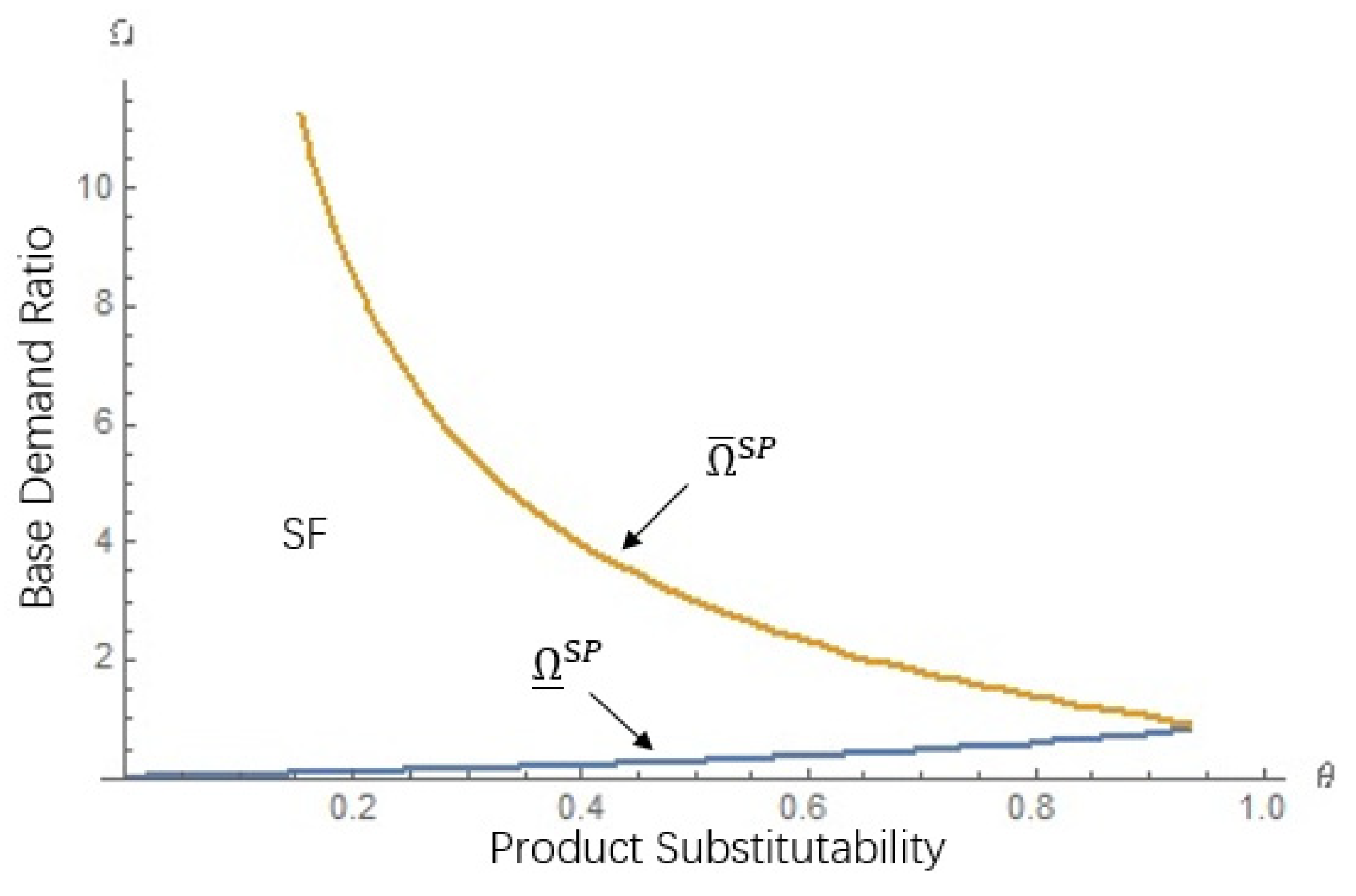
Under supplier-led innovation, in both the SF and SP situations, the supplier benefits from its own innovation; therefore, it has an incentive to innovate. In addition, the SF situation is better than SP for the supplier and only if ${\underset{\_}{\Omega }}^{SP}\left(\theta \right)<\Omega <{\overline{\Omega }}^{SP}\left(\theta \right)$.

Proposition 1 reflects the conventional wisdom that the supplier is rewarded for its own innovation. Because new technological experience will stimulate consumers’ desire to buy, the supplier’s innovation generates more demand for its own product. Therefore, innovation is the main equilibrium strategy of the supplier. It also suggests that SF always performs better than does SP in the feasible region. With the increase of product substitutability, the supplier still chooses SF because when the products in all channels are updated, here, SF significantly increases the supplier’s own demand, so the supplier finds that SF is beneficial, as illustrated in Figure 1. The practical insight for the supplier is that it should sufficiently innovate its products for each channel, and this is even more important for a channel with a smaller base market.

3.3. M-Model

In this section, we will investigate the M-Model, in which the manufacturer innovates and the supplier does not. Moreover, this model is divided into an only one manufacturer-led innovation system model (MO) and a both manufacturer-led innovation system model (MB). In the MO-Model, only one channel of manufacturers chooses to create the products, and under the MB-Model, the manufacturers from both channels create their products.

In only one manufacturer-led innovation system model (MO), the new base demand and profit functions of the supplier and manufacturers are then, respectively:

$$a_i=A_i+\left(2-i\right) e_{mi} ,i=1,2,$$

(12)

$${\pi }_s^{MO}={\displaystyle \sum }_{i=1}^2(D_i\ast w_i) ,i=1,2,$$

(13)

$${\pi }_{mi}^{MO}=D_i\ast \left(p_i-w_i\right)-\left(2-i\right)\ast {\eta }_m\ast e_{mi}{}^2, i=1,2.$$

(14)

Lemma 4.

The results show that ${\pi }_{m1}^{MO}>{\pi }_{m1}^B$ if and only if ${\hat{\Omega }}_{m1}^{MO-B}<\Omega <{\overline{\Omega }}^{MO}$ by comparing the profits of manufacturer1 under the MO-Model and the B-Model.

Lemma 4 provides that the manufacturer will get more profits than the basic model under the premise that the opponent does not innovate. Therefore, the manufacturer has the motivation to innovate.

In the both manufacturer-led innovation system model (MB), the new base demand and profit functions of the supplier and manufacturers are then, respectively:

$$a_i=A_i+e_{mi},$$

(15)

$${\pi }_s^{MB}={\displaystyle \sum }_{i=1}^2(D_i\ast w_i) ,i=1,2,$$

(16)

$${\pi }_{mi}^{MB}=D_i\ast \left(p_i-w_i\right)-{\eta }_m\ast e_{mi}{}^2, i=1,2.$$

(17)

Lemma 5.

The results show that ${\pi }_{m2}^{MB}>{\pi }_{m2}^{MO}$ if and only if ${\underset{\_}{\Omega }}^{RB}<\Omega <{\hat{\Omega }}_{m2}^{RB-RO}$, by comparing the profits of manufacturer1 under the MO-Model and the MB-Model.

Lemma 5 provides that when manufacturers innovate products based on market demand, they will stimulate consumers’ desire to buy and increase product sales. When sales reach a certain level, increasing profits and innovation costs will be ignored.

Proposition 2.

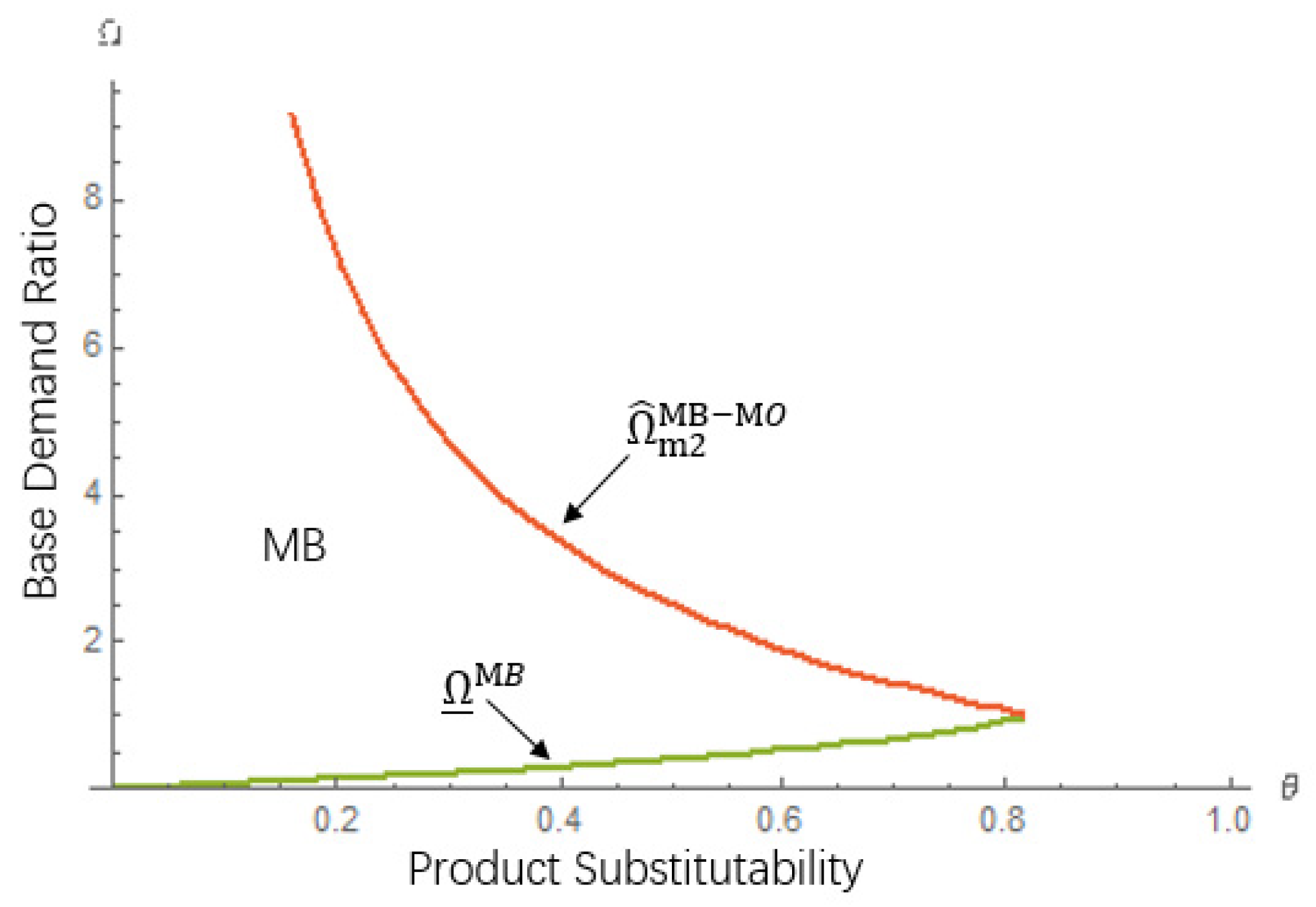
Under manufacturer-led innovation, one of the manufacturers benefits from its own innovation when its rival does not innovate if and only if ${\hat{\Omega }}_{m1}^{MO-B}\left(\theta \right)<\Omega <{\overline{\Omega }}^{MO}\left(\theta \right)$; therefore, there is an incentive for a manufacturer to innovate; the other manufacturer also benefits by choosing to innovate when its rival innovates if and only if ${\underset{\_}{\Omega }}^{MB}\left(\theta \right)<\Omega <{\hat{\Omega }}_{m2}^{MB-MO}\left(\theta \right)$; likewise, there is an incentive for the other one to innovate.

Proposition 2 implies that a manufacturer can still gain extra profits from its own innovation, as illustrated in Figure 2 and Figure 3. When the other manufacturer has no product innovation, one of the manufacturers actively drives product innovation, which will stimulate the consumers’ desire to buy and expand the market demand of its channel, thus increasing profits. In addition, with the increase of $\theta$, one manufacturer will gradually occupy the product market of the other one; therefore, there will be more profit space. Under the incentive of one of the manufacturers’ innovation, the other manufacturer also creates the products in its own channel. At this time, the other one is in the supply chain with smaller base market, and it faces the prospect of gaining from its own innovation insufficient incremental profit to compensate for the innovation costs incurred. The practical implication for manufacturers is that to occupy the basic consumer market space, manufacturers should take the initiative to drive market innovation, and in the case of high product substitutability, they should increase innovation efforts to continuously expand market share on the premise of maintaining market share. Manufacturers should also benefit from taking action rather than waiting for their market to be taken when a competitor innovates.

4. Supply Chain Efficiency

This section contains other performance indicators, in particular total supply chain profits, not individual company profits and consumer welfare. The closed-form solutions of pricing decisions and demands are as follows.

For the supply chain profit comparison, we define the supply chain efficiency as the sum of all members’ profits, and the comparison results are shown in the following proposition.

Proposition 3.

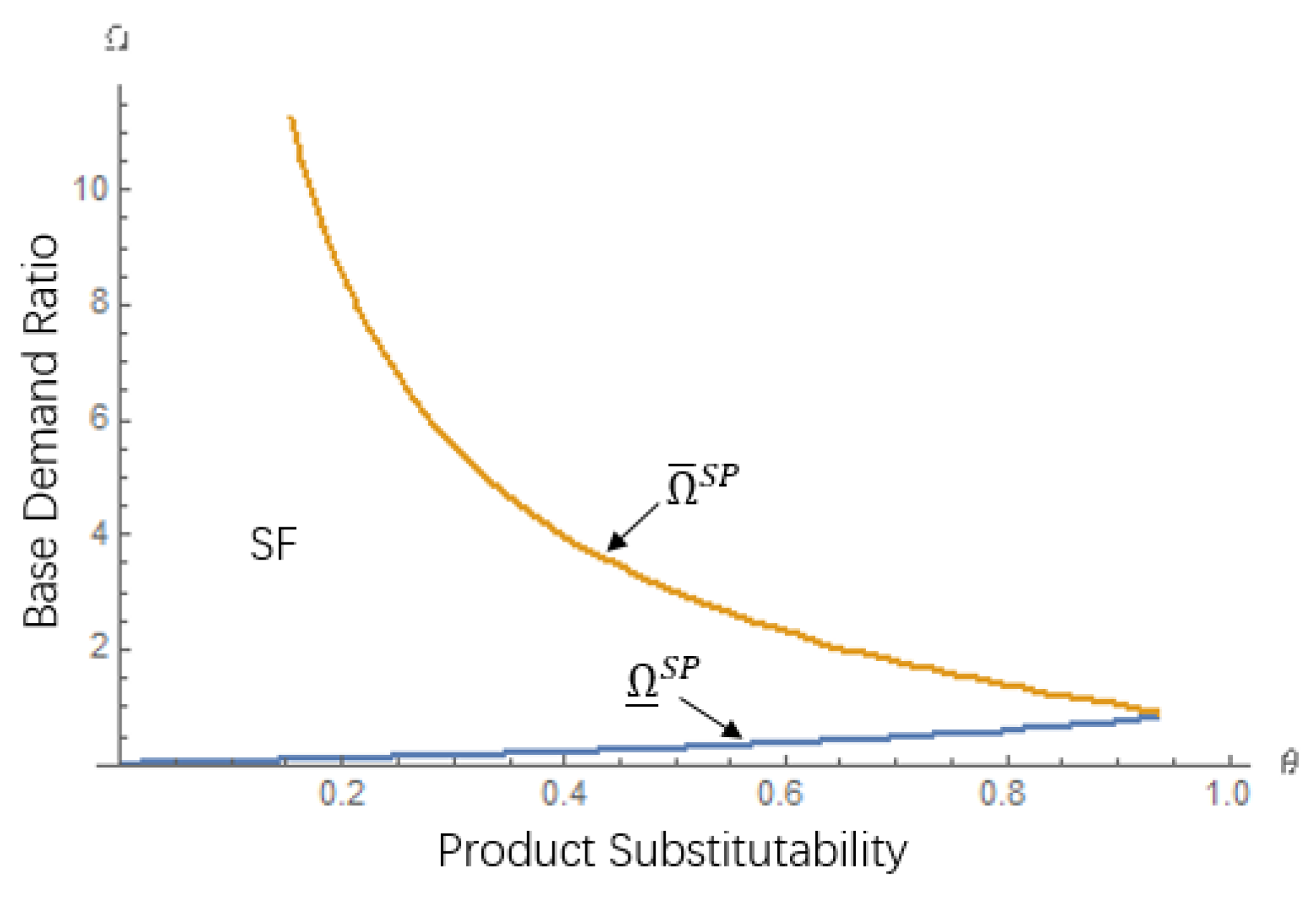
($i$) In a supplier-led innovation system, a supply chain gains more profits from an SF strategy than from an SP strategy if and only if ${\underset{\_}{\Omega }}^{SP}\left(\theta \right)<\Omega <{\overline{\Omega }}^{SP}\left(\theta \right)$; ($ii$) in a manufacturer-led innovation system, a supply chain gains more profits from an MB strategy than from an MO strategy if ${\underset{\_}{\Omega }}^{MB}\left(\theta \right)<\Omega <{\underset{\_}{\Omega }}^{MB-MO}\left(\theta \right)$, and it gains more profits from an MO strategy than from an MB strategy if ${\underset{\_}{\Omega }}^{MB-MO}\left(\theta \right)<\Omega <{\overline{\Omega }}^{MB-MO}\left(\theta \right)$.

Proposition 3 shows that in a supplier-led innovation system, more profit will be obtained under an SF innovation strategy than under an SP innovation strategy for the supply chain, as illustrated in Figure 3. This means that when supplier drives product innovation across all channels, he will gain more market share, sell more products, and will maximize the overall profit of the entire supply chain. In a manufacturer-led innovation system, the supply chain will have different choices in different feasible intervals. When the product substitutability is the same and the basic market of different manufacturers varies greatly, the supply chain will choose the MO innovation strategy; otherwise, the supply chain will choose the MB innovation strategy. This shows that when the difference between the basic market shares of manufacturers is large, the manufacturer with a large share of the basic market can only be selected for innovation, and the manufacturer with a small share of the basic market can be ignored in the supply chain: this will reduce the innovation cost. The practical significance is that for the supply chain, to obtain the most profit, it is not necessary to create the products of all channels. In contrast, sometimes ignoring the products with a small proportion of the basic market share will reduce the innovation cost.

Corollary 1.

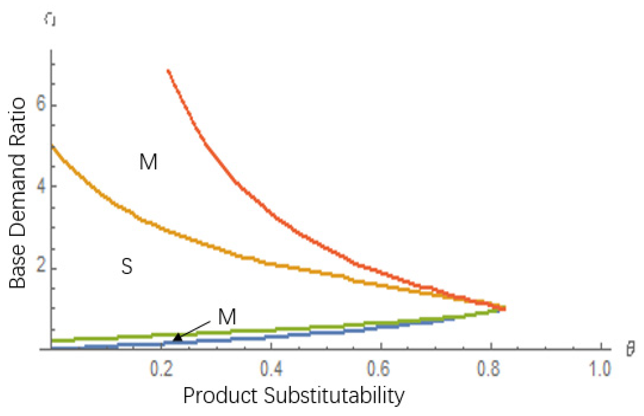
For a supply chain, a supplier-led innovation system performs better than a manufacturer-led innovation system if and only if ${\underset{\_}{\Omega }}^{SF-MB}\left(\theta \right)<\Omega <{\overline{\Omega }}^{SF-MB}\left(\theta \right)$; a manufacturer-led innovation system performs better than a supplier-led innovation system if ${\underset{\_}{\Omega }}^{MB}\left(\theta \right)<\Omega <{\underset{\_}{\Omega }}^{SF-MB}\left(\theta \right)$ and ${\overline{\Omega }}^{SF-MB}\left(\theta \right)<\Omega <{\overline{\Omega }}^{MB-MO}\left(\theta \right)$.

Corollary 1 implies that the supply chain will choose different innovation systems in different value ranges, as illustrated in Figure 4, Figure 5 and Figure 6. For the same level of product substitutability, the basic market of different manufacturers varies greatly or little. Therefore, the supply chain will choose the M innovation system; otherwise, the supply chain will choose the S innovation system. The practical significance of this is that when the market of different product brands is different or basically equal, the manufacturer is closer to the consumer market and the revenue generated by product innovation driven by it is better. When the differences in brand markets are small, to drive product innovation that benefits the entire supply chain, the supplier can use their ability to dominate.

5. Consumer Welfare

Consumer welfare is denoted by $U$, and the subscript indicates the innovative structure being used; it represents the utility of consumers. For any parameters pair $\left(\theta , \Omega \right)$ in a common feasible area, the innovative structures can be sorted as follows.

Proposition 4.

The innovation structure produces consumer welfare results in the following relative order:$U_{MB}>U_{SF},$ and $U_{MO}>U_{SP}>U_B$.

Proposition 4 shows that consumers can obtain more utility from the manufacturer innovation because this type of innovation can induce greater competition and lowers retail prices consequently (and generates bigger consumption than does supplier innovation). For asymmetric channels, under manufacturer innovation, the retail price in the supply chain is lower than the retail price in supplier innovation. In addition, it also shows that manufacturers understand the needs of the end consumer market better than suppliers. Manufacturers’ innovative products can enable consumers to have a better shopping experience. We know that the essence of innovation is that innovation itself can benefit consumers in some ways different from the price and the total consumption. For example, more innovation can be achieved by providing newer products or a better consumer experience.

6. Conclusions

This paper investigates the efficacy of supplier innovation and manufacturer innovations in a dual channel model with competing supply chains. In addition, it develops three innovation models, including the B-Model, the S-Models, and the M-Models. Our results show managerial insights to better understand in practice some kinds of innovation strategies. We derive that the supplier has an incentive to innovate in the market; however, the innovation of products from all channels will bring more profits to supplier. When no manufacturer creates the product, one of them will obtain a good profit from the innovation, and in the face of the innovation of competitors, the other manufacturers will have the incentive to innovate. For the supply chain, in a supplier-led system, an SF strategy is a better strategy. In a manufacturer-led system, the MB and MO strategies will be selected differently in different regions, to obtain the most profit, it is not necessary to create the products of all channels. Another interesting conclusion is that under the same level of product substitutability, when the difference in the basic markets is not large, a supplier-led system is a better choice. Otherwise, a manufacturer-led system is a better choice. Through comparison, it is found that the utility under a manufacturer-led system is the largest. This also confirms that the manufacturer is more aware of the market demand than is the supplier. Our research provides a reasonable explanation and choice of innovative strategies for the phenomenon that upstream and downstream are competing for battery innovation in the electric vehicle field. The practical significance of this article is that for manufacturers and the supplier, how to choose the corresponding innovation strategy when facing the market and want to make innovations will make themselves more profitable.

Compared with the paper on supply chain innovation, this paper focuses on which of the downstream manufacturers’ corresponding market innovation drivers and upstream suppliers’ corresponding technological innovation drivers is better for the supply chain, and for manufacturers and suppliers [28]. When facing the market demand, whether active innovation will make more profits. He considers the cost-sharing game model in which manufacturers incentivize suppliers to innovate in a supply chain system composed of one supplier and two manufacturers under the full cooperation, semi-cooperation and non-cooperation of the manufacturer, and study the effect of downstream interactive behavior on incentive contracts and the influence of upstream suppliers’ innovation decisions. The nodes studied in the two articles are different, this paper does not consider the influence of the relationship between downstream manufacturers on supplier innovation. Therefore, the conclusions reached also have great limitations and this can be used as the direction of a future paper.

Our work also provides a model for learning how the channel structure interacts with similar decisions around innovation and other similar market development activities. Future research could include the analysis of the influence on the conclusion of the paper, of changing the value of the parameters Ω. A challenge in this regard is obtaining analytical results, as the problems will become more complicated to resolve. Furthermore, we can consider other issues, including the effect of product substitutability on the above conclusions. Finally, additional research might also consider the impact on the above conclusions of changes in the cost sharing ratio in different situations.

References

- Wong, D.T.; Ngai, E.W. Critical Review of Supply Chain Innovation Research (1999–2016). Ind. Mark. Manag. 2019, 82, 158–187. [Google Scholar] [CrossRef]
- Schumpeter, J.A. The Theory of Economic Development: An Inquiry into Profits, Capital, Credit, Interest, and the Business Cycle; Harvard University Press: Cambridge, MA, USA, 1934; ISBN 9780674879904. [Google Scholar]
- Gao, D.; Xu, Z.; Ruan, Y.Z.; Lu, H. From a Systematic Literature Review to Integrated Definition for Sustainable Supply Chain Innovation (Ssci). J. Clean. Prod. 2017, 142, 1518–1538. [Google Scholar] [CrossRef]
- Bruce, M. Dangerous Liaisons: An Application of Supply Chain Modelling for Studying Innovation within the UK Clothing Industry. Technol. Anal. Strateg. Manag. 1999, 11, 113–125. [Google Scholar] [CrossRef]
- Yan, T.; Dooley, K.; Thomas, Y.C. Measuring Supplier Innovation. Supply Chain Manag. Rev. 2018, 22, 38–45. [Google Scholar]
- Jean, R.J.B.; Sinkovics, R.R.; Hiebaum, T.P. The Effects of Supplier Involvement and Knowledge Protection on Product Innovation in Customer-Supplier Relationships: A Study of Global Automotive Suppliers in China. J. Prod. Innov. Manag. 2014, 31, 98–113. [Google Scholar] [CrossRef]
- Liker, J.K.; Kamath, R.R.; Wasti, S.N.; Nagamachi, M. Supplier involvement in automotive component design: Are there really large US Japan differences? Res. Policy 1996, 25, 59–89. [Google Scholar] [CrossRef]
- Petersen, K.J.; Handfield, R.B.; Ragatz, G.L. A Model of Supplier Integration into New Product Development. J. Prod. Innov. Manag. 2003, 20, 284–299. [Google Scholar] [CrossRef]
- Kim, M.; Chai, S. The impact of supplier innovativeness, information sharing and strategic sourcing on improving supply chain agility: Global supply chain perspective. Int. J. Prod. Econ. 2017, 187, 42–52. [Google Scholar] [CrossRef]
- Chae, S.; Yan, T.; Yang, Y. Supplier innovation value from a buyer-supplier structural equivalence view: Evidence from the PACE Awards in the automotive industry. J. Oper. Manag. 2019, 1–19. [Google Scholar] [CrossRef]
- Pihlajamaa, M.; Kaipia, R.; Aminoff, A.; Tanskanen, K. How to stimulate supplier innovation? Insights from a multiple case study. J. Purch. Supply Manag. 2019, 25, 100536. [Google Scholar] [CrossRef]
- Zhang, J. R&D for Environmental Innovation and Supportive Policy: The Implications for New Energy Automobile Industry in China. Energy Procedia 2011, 5, 1003–1007. [Google Scholar] [CrossRef] [Green Version]
- Trautrims, A.; MacCarthy, B.L.; Okade, C. Building an innovation-based supplier portfolio: The use of patent analysis in strategic supplier selection in the automotive sector. Int. J. Prod. Econ. 2017, 194, 228–236. [Google Scholar] [CrossRef] [Green Version]
- Potter, A.; Graham, S. Supplier involvement in eco-innovation: The co-development of electric, hybrid and fuel cell technologies within the Japanese automotive industry. J. Clean. Prod. 2019, 210, 1216–1228. [Google Scholar] [CrossRef] [Green Version]
- Zhu, K.; Zhang, R.Q.; Tsung, F. Pushing Quality Improvement along Supply Chains. Manag. Sci. 2007, 53, 421–436. [Google Scholar] [CrossRef]
- Gilbert, S.M.; Cvsa, V. Strategic Commitment to Price to Stimulate Downstream Innovation in a Supply Chain. Eur. J. Oper. Res. 2003, 150, 617–639. [Google Scholar] [CrossRef]
- Chang, X.X.; Shen, F.P. Strategic Commitment to Price in a Supply Chain with Downstream Innovation. Open J. Bus. Manag. 2019, 7, 1690–1704. [Google Scholar] [CrossRef] [Green Version]
- Erzurumlu, S. Collaborative Product Development with Competitors to Stimulate Downstream Innovation. Int. J. Innov. Manag. 2010, 14, 573–602. [Google Scholar] [CrossRef]
- Talluri, S.; Narasimhan, R.; Chung, W. Manufacturer cooperation in supplier development under risk. Eur. J. Oper. Res. 2010, 207, 165–173. [Google Scholar] [CrossRef]
- Wang, J.; Shin, H. The Impact of Contracts and Competition on Upstream Innovation in a Supply Chain. Prod. Oper. Manag. 2015, 24, 134–146. [Google Scholar] [CrossRef]
- Ma, P.; Wang, H.; Shang, J. Supply chain channel strategies with quality and marketing effort-dependent demand. Int. J. Prod. Econ. 2013, 144, 572–581. [Google Scholar] [CrossRef]
- Friedl, G.; Wagner, S.M. Supplier development investments in a triadic setting. IEEE Trans. Eng. Manag. 2016, 63, 136–150. [Google Scholar] [CrossRef]
- Chen, Y.; Joshi, Y.V.; Raju, J.S.; Zhang, Z.J. A theory of combative advertising. Mark. Sci. 2009, 28, 1–19. [Google Scholar] [CrossRef] [Green Version]
- Tsay, A.A.; Agrawal, N. Channel dynamics under price and service competition. Manuf. Serv. Oper. Manag. 2000, 2, 372–391. [Google Scholar] [CrossRef]
- Ingene, C.A.; Parry, M.E. Mathematical Models of Distribution Channels; Kluwer Academic Publishers: Dordrecht, The Netherlands, 2004; ISBN 1-4020-7163-9. [Google Scholar]
- Ingene, C.A.; Parry, M. Bilateral monopoly, identic al competitors/distributors, and game theoretic analyses of distribution channels. J. Acad. Mark. Sci. 2007, 35, 586–602. [Google Scholar] [CrossRef]
- Liu, B.; Cai, G.; Tsay, A.A. Advertising in Asymmetric Competing Supply Chains. Prod. Oper. Manag. 2014, 23, 1845–1858. [Google Scholar] [CrossRef]
- Liu, C. The Decision Analysis and Contract Design of Manufacturers Stimulating Supplier Innovation; Huazhong University of Science and Technology: Wuhan, China, 2018; pp. 40–79. [Google Scholar]
Figure 1.
Supplier’s profit comparison between SF and SP.
Figure 2.
Manufacturer profit comparison between MO and B.
Figure 3.
Manufacturer profit comparison between MB and MO.
Figure 4.
Supply chain’s profit comparison between MB and MO.
Figure 5.
Supply chain’s profit comparison between SF and SP.
Figure 6.
Supply chain’s profit comparison between S and M.