Crash Risk Assessment for Heterogeneity Traffic and Different Vehicle-Following Patterns Using Microscopic Traffic Flow Data

Abstract

This paper investigates the impacts of heavy vehicles (HV) on speed variation and assesses the rear-end crash risk for four vehicle-following patterns in a heterogeneous traffic flow condition using three surrogate safety measures: speed variation, time-to-collision (TTC), and deceleration rate to avoid a crash (DRAC). A video-based data collection approach was employed to collect the speed of each individual vehicle and vehicle-following headway; a total of 3859 vehicle-following pairs were identified. Binary logistic regression modeling was employed to assess the impacts of HV percentage on crash risk. TTCs and DRACs were calculated based on the collected traffic flow data. Analytical models were developed to estimate the minimum safe vehicle-following headways for the four vehicle-following patterns. Field data revealed that the variation of speed first increased with HV percentage and reached the maximum when HV percentage was at around 0.35; then, it displayed a decreasing trend with HV percentage. Binary logistic regression modeling results suggest that a high risk of rear-end collision is expected when HV percentage is between 0.19 and 0.5; while, when HV percentage is either below 0.19 or exceed 0.5, a low risk of rear-end collision is anticipated. Analytical modeling results show that the passenger car (PC)-HV vehicle-following pattern requires the largest minimum safe space headway, followed by HV-HV, PC-PC, and HV-PC vehicle-following patterns. Findings from this research present insights to transportation engineers regarding the development of crash mitigation strategies and have the potential to advance the design of real-time in-vehicle forward collision warnings to minimize the risk of rear-end crash.

1. Introduction

In China and many other developing countries, it has been a common phenomenon that passenger car (PC) driving is mixed with heavy vehicles (HVs), i.e., trucks and buses, on both freeways and arterials [1,2,3], which is defined as heterogeneous traffic flow. This is mainly because public transport, such as inner-city buses and intercity coaches, can carry more passengers in comparison with PCs and thus has the potential to relieve traffic congestion problems [4,5,6]. Moreover, trucks are the primary land freight transport mode in the logistic chain and transfer freight to and from seaports, airfields, rail terminals, etc. [7,8]. This kind of heterogeneous traffic flow characteristic, however, has been regarded as one of the primary reasons for traffic collision [9,10,11,12,13,14]. When traffic volume is low, PC drivers usually drive at a relatively higher speed than HV drivers and tend to overtake a leading HV. In comparison, under high traffic volume conditions, because there are no sufficient overtaking opportunities, under the majority of situations a driver has to follow the leading vehicle [15,16]. Nevertheless, in reality, it was found that the variety in vehicle-following patterns (i.e., a PC following another passenger vehicle, PC-PC; a PC following a HV, PC-HV; a HV following a PC, HV-PC; and a HV following another HV, HV-HV) resulted in potential variations in speed and headway in traffic flow [17,18,19,20,21]. In addition, during the vehicle-following process, the following vehicle driver has to adjust his or her driving behavior, such as following headways, acceleration and deceleration maneuvers, and lane-changing decisions based on the status of the leading vehicle [22,23,24,25]. Considering the aggressive driving behaviors in China, such as the short vehicle-following headway and the frequent acceleration and deceleration maneuvers, the turbulences in traffic flow could be further deteriorated [14,26].

Due to the heterogeneities in both vehicle dynamics and drivers’ driving experience and behavior, the various vehicle-following patterns tend to result in variations in speed and/or time headway, which increase the potential of rear-end collisions [27]. In a real-world setting, the sightline of PC drivers is relatively low (approximately 1.1 m above the road surface) and typically parallel to the road. In comparison, the sightline of HV drivers is significantly higher than PC drivers (approximately 2.5 m above the road surface) and, usually, HV drivers tend to look down at the road due to the relative high sightline [28,29]. The difference in driving postures would affect the view of drivers and their estimations of the space headway to the leading vehicle. Generally speaking, HV drivers tend to overestimate space headways, which increases the risk of rear-end collisions [30].

With this concern, it is necessary to take into account the impacts of vehicle characteristics and driving behavior on traffic operations when assessing the risk of crashes on freeways. In this regard, this research aims to investigate the risks of rear-end crashes for different vehicle-following patterns based on microscopic real-world traffic flow data; accordingly, it could provide recommendations to drivers regarding the potential crash risk and minimum safe vehicle-following headways, so that they can timely adjust their driving behavior to reduce the possibility of being involved in a rear-end crash. The remainder of this paper is organized as follows: Section 2 presents a review of the start-of-the-art regarding crash risk assessment. Section 3 describes the acquisition and reduction of vehicle-type-specific traffic flow data. Section 4 details the methodologies employed for assessing the crash risk under different vehicle-following patterns. Section 5 documents the minimum safe vehicle-following distances for each vehicle-following pattern. Finally, the conclusions of this study and discussions on future research requirements are summarized in Section 6.

2. Literature Review

To date, there have been a number of studies that employed real-world traffic flow data for crash risk assessment. Oh et al. [31] identified rear-end collision risks based on traffic flow data collected by inductive loop detectors. Traffic performance data of individual vehicles were extracted from loop detectors, which were employed to identify collision potentials. Similarly, Abdel-Aty et al. [32] identified crash-prone conditions on freeways using loop detector data. Logistic regression models were developed for assessing the risk of crashes under two different speed conditions. It was concluded that the crashes that occur under moderate- to high-speed condition differ distinctly from low-speed condition in both severity and traffic flow conditions. Shew et al. [33] also employed loop detector data to estimate real-time crash risks on freeways. The classification tree and neural network-based crash risk assessment models were developed, and they are expected to provide local authorities with a reasonable estimate of crash risk. Yu and Abdel-Aty [34] utilized the support vector machine (SVM) model to evaluate real-time crash risk. Results indicated that SVM models have great application potential in real-time crash risk evaluation because they require a smaller sample size than the traditional logistic regression models to generate a comparable result. Lao et al. [35] developed a generalized nonlinear model (GNM) for estimating highway rear-end crash risk. Rear-end accident data collected from 10 highway routes in the state of Washington were employed to calibrate the model. Results suggested that truck percentage and grade increased crash risks initially but decreased the risks after reaching certain thresholds. Kwak and Kho [36] developed real-time crash risk prediction models for different expressway segment types (mainline and ramp) and traffic flow states (uncongested and congested). Modeling results showed that both roadway type and traffic flow characteristics influenced the predicted crash risks. Yu et al. [37] developed disaggregate crash risk analysis models with loop detector traffic data and historical crash data to reveal the mechanisms of crashes. Through a Bayesian semi-parametric model, it was found that crashes occurring during weekday peak hours were impacted by upstream traffic; variations of volume and the speed drops would increase crash occurrence likelihood. Mullakkal-Babu et al. [38] presented a qualitative and quantitative comparison of five safety indicators (i.e., inverse time to collision, post-encroachment time, potential indicator of collision with urgent deceleration, warning index, and safety field force) to evaluate their usefulness in quantifying crash risks. Results indicated that all five safety indicators were capable of delineating risk continuously in a one-dimensional interaction such as car-following. Xu et al. [1] investigated the impacts of traffic flow conditions on the casualty of different collision types based on high-resolution traffic data. Based on logistic regression modeling, it was found that, for sideswipe crashes, the crash risk was influenced by the speed difference between adjacent lanes, volume on the right lane, and standard deviation of volume on inner lanes. For rear-end crashes, the congested traffic conditions at the diverge area, and a large difference in speed on the right lane between the upstream and downstream stations in adverse weather, contributed to crash casualty.

For heterogeneous traffic flow conditions, several studies have been conducted to investigate the heterogeneity in vehicle-following behavior, as well as its impact on crash risk. Ossen and Hoogendoorn [19] identified the different vehicle-following behaviors of passenger vehicle and truck drivers. Results suggested that the desired headways of passenger car drivers were lower when following a truck than when following a passenger car. In comparison, truck drivers adopted a more conservative vehicle-following behavior than passenger vehicle drivers did, and their speed variations were lower than those of passenger vehicle drivers. Ye and Zhang [29] investigated four vehicle type-specific time headways based on different combinations of leading vehicles and following vehicles at different traffic flow levels. Statistical results revealed that, under all traffic flow conditions, the truck-truck headway was the largest and the car-car headway was the smallest. The truck-car headway was larger than the car-truck headway, which is mainly because truck drivers are usually sitting higher than car drivers, which enables them to look beyond the car they are following, and thus keep a smaller separation. Furthermore, it was found that traffic flow level affected vehicle type-specific headway characteristics. Weng et al. [20] evaluated rear-end crash risk in work zones for four different vehicle-following patterns. Results show that the car-truck following pattern had the largest rear-end crash risk, followed by truck-truck, truck-car, and car-car patterns. Recently, Hyun et al. [39] employed the headways obtained from inductive loop detectors to investigate the impacts of trucks on crash risk. A Gaussian Mixture (GM) model was developed to identify trucks and analyze the interactions between trucks and non-trucks. Modeling results revealed that interactions between the leading and following vehicles were significantly associated with crash risk; rear-end crashes were more likely to occur when a truck was following a non-truck. Therefore, traditional safety measures that estimate the average traffic condition such as total volume or average headway of the traffic stream might not exactly capture the actual crash risk. Zhao and Lee [40] analyzed the rear-end collision risk of cars and heavy vehicles on freeways using crash potential index (CPI) as the surrogate measure of safety (SMoS). It was found that rear-end collision risk was lower for heavy vehicles than for cars in the crash case due to their shorter reaction time and lower speed when space headway was shorter. With this consideration, the authors emphasized the importance of reflecting the differences in driver behavior and vehicle performance characteristics between cars and heavy vehicles when estimating crash risk. Dimitriou et al. [21] investigated car-following characteristics and vehicle-by-vehicle interactions to assess rear-end crash potential on urban roads. The stopping distance between two consecutive vehicles was employed as a SMoS. It was found that speeds were lower and headways were higher when trucks lead; moreover, rear-end crash potential was presented when traffic flow and speed standard deviation was higher. Similarly, Choudhary et al. [41] explored the relationships of speed variations between different vehicle types with crashes through a Multivariate Poisson lognormal regression model. Modeling results revealed that crash rates increased with the raise of speed variations, especially at higher traffic volumes. In addition, modeling results suggested that specific combinations of traffic characteristics increase the likelihood of crashes. Mahmud et al. [3] investigated the factors affecting crash frequency on a two-lane two-way highway in a heterogeneous traffic environment using micro-level traffic flow data; accordingly, he identified the safety risk locations of a particular road section. It was concluded that speeding was the primary influential factor in crashes. Zhang et al. [2] pointed out that a driver’s car-following behavior depends on perceived risk levels, acceleration and deceleration habits, and driver reaction characteristics. Based on this, the authors investigated the impact of heterogeneity of driving behavior on rear-end crash risk through simulation experiments. Simulation results implied that driving behavior characteristics and the proportion of different driving styles (i.e., stable and unstable driving styles) were the most critical factors that affect shock waves in traffic flow, and subsequently rear-end crash risk. When stable and unstable driving styles coexist, their proportions had important influences on rear-end crash risk.

In summary, previous research generally revealed that driving behavior heterogeneity has a considerable impact on rear-end crash risk. Therefore, exploring the effect of each vehicle-following behavior on rear-end crash probability could improve our understanding of crash risk and would support the development of more efficient safety countermeasures to minimize rear-end crash risks.

3. Data Acquisition

3.1. Data Collection and Reduction

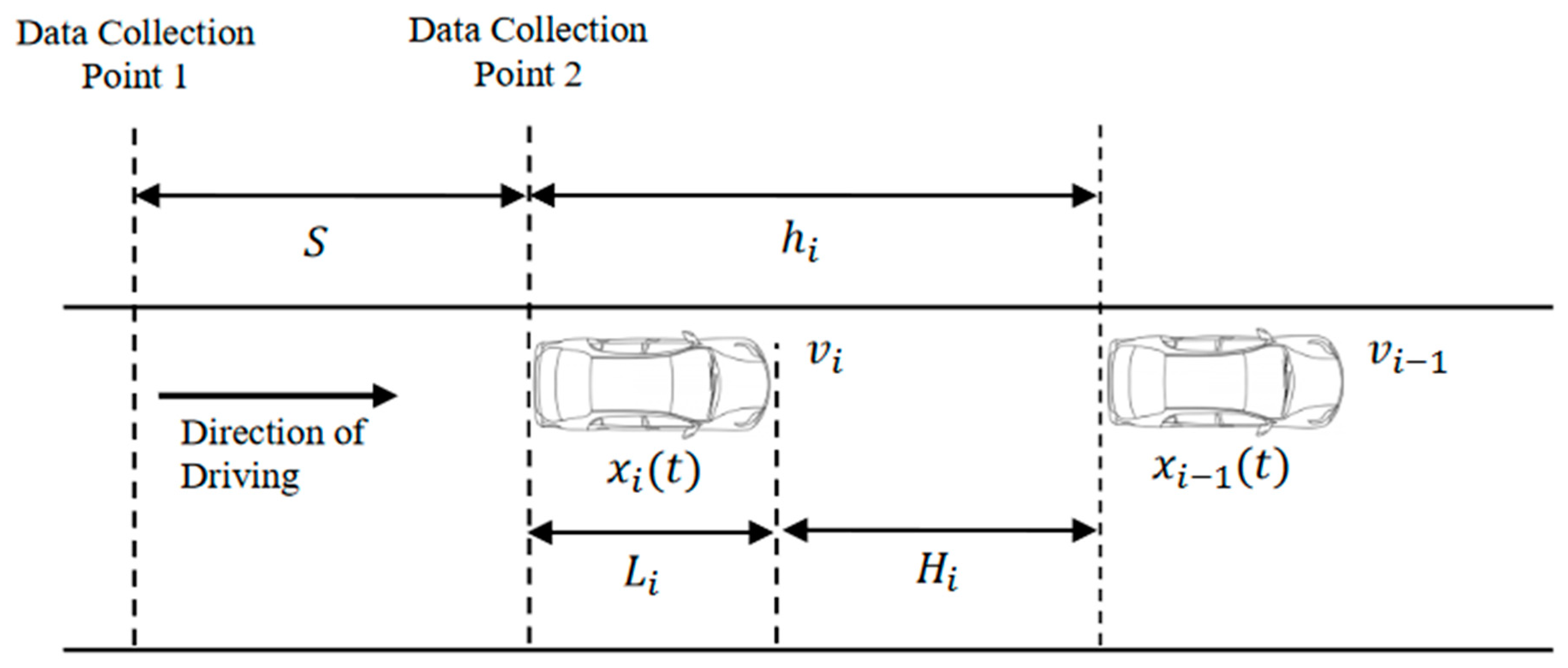
Real-world microscopic traffic flow data, including traffic volume, traffic composition (i.e., percent of HVs), speed and variations of speed, and time and space headways were collected at a representative freeway (i.e., freeway S-28) in Yangzhou City, China, using video cameras. Figure 1 illustrates the location and method for data collection. The data collection was conducted on weekdays under normal weather condition. To cover a variety of traffic flow conditions, traffic performance data under both peak and non-peak periods were collected.

To extract traffic flow data on each lane, this research first defined the left-most lane as the passing lane (Lane 1), the middle lane as the driving lane (Lane 2), and the right-most lane as the merging lane (Lane 3). Then, this research used codes 1 and 2 to represent passenger vehicles and heavy vehicles, respectively. Based on the vehicle classification standard in China [42], this research defined passenger vehicles as vehicles with a length of less than 6 m. Vehicles that have a length of 6 m or longer were defined as heavy vehicles.

The spot speed of each vehicle was extracted based on the time (in the number of frames) passing a designated distance, which was determined as 30 m, as shown in Figure 1. In addition, time and speed headways and speed variations of each paired sample were extracted from the video clips. The procedure for data extraction is illustrated in Figure 2. This video-based speed data processing approach can provide a higher speed-data measurement accuracy and has the flexibility to retrieve detailed vehicle-following trajectories of each paired sample [43]. Details of the microscopic traffic flow data extraction procedure are described as follows:

Spot speed of each vehicle:

$$v_i\left(t\right) = \frac{S}{b_{i,2}-b_{i,1}}\times k$$

(1)

where:

• $v_i\left(t\right)$ is the spot speed (m/s) of vehicle $i$ at time point $t$;
• $S$ is the distance between observation points 1 and 2, which was defaulted as 30 m;
• $b_{i,1}$ and $b_{i,2}$ are the frame number at observation points 1 and 2, respectively;
• $k$ is the number of frames per second, which was 25 frames per second (i.e., 0.04 s per frame).

Time headway of each paired sample:

$$t_{i }=b_{i,1}-b_{i-1,1}\times k$$

(2)

where:

• $t_i$ is the time headway (s) of each paired sample;
• $b_{i,1}$ and $b_{i-1,1}$ are the frame number of the tail of vehicles $i$ and $i-1$ passing observation point 1, respectively;
• $k=0.04$.

Space headway (m) of each paired sample:

$$h_i=v_i\left(t\right)\times k$$

(3)

Vehicle length (m):

$$L_i=\left(b_{i,1}^{\prime }-b_{i,1}\right)\times k\times v_i\left(t\right)$$

(4)

where:

$L_i$ 

is the length of each vehicle;

$b_{i,1}^{’}$ 

and $b_{i,1}$ are the frame number of the tail and bumper of vehicles $i$ passing  observation point 1, respectively.

Space interval (m) between paired vehicles, which is the distance between the tail of the leading vehicle and bumper of the following vehicle:

$$H_i=h_i-L_i$$

(5)

Speed difference (m/s) of each paired sample:

$$\delta v =v_i-v_{i-1}$$

(6)

where:

• $\delta v$ is the speed difference of vehicles $i$ (following vehicle) and $i-1$ (leading vehicle);
• $v_i$ and $v_{i-1}$ are the speeds of vehicles $i$ and $i-1$, respectively.

An example of the extracted individual vehicle speed information is illustrated in

Table 1. Examples of the Data Extraction Procedure and Extracted Traffic Data.

Vehicle #	Time	Frame #			Vehicle Type	Lane #	Vehicle Length (m)	Distance (m)	Spot Speed (km/h)
		Head at Location 1	Rear at Location 1	Rear at Location 2
1	7:07:48	n/a	11,838	11,862	11	1	5	30	112.5
2	7:07:59	12,100	12,125	12,157	21	2	23	30	84.4
3	…	…	…	…	…	…	…	…	…

Note: # refers to number.

.

3.2. Descriptive Statistics

Based on the aforementioned video-based data extraction procedure, full data extraction was performed. Descriptive statistics of traffic flow and travel speed are listed in

Table 2. Traffic Flow Data Extracted from the Video Clips.

Lane	Passenger Vehicle (PV)		Heavy Vehicle (HV)		Total
	Traffic Volume	Percentage (%)	Traffic Volume	Percentage (%)
Passing Lane	4948	91.9	438	8.1	5386
Driving Lane	2748	72.5	1040	27.5	3788
Merging Lane	1239	93.3	89	6.7	1328
Total	8935	85.1	1567	14.9	10,502

and

Table 3. Travel Speeds Extracted from the Video Clips.

Lane	Vehicle Type	Sample Size	Speed (km/h)				Low Speeds	High Speeds
			Mean	S.D.	15%	85%
Passing Lane	PV	4948	96.3	10.73	87.1	108.0	12.6%	15.0%
	HV	438	90.7	10.06	79.4	100.0	13.0%	26.5%
Driving Lane	PV	2748	82.5	18.35	61.4	203.9	12.2%	10.2%
	HV	1040	79.1	11.59	67.5	90.0	15.6%	19.8%
Merging Lane	PV	1239	61.7	9.02	52.9	69.2	11.8%	20.9%
	HV	89	55.8	8.97	47.0	64.3	14.6%	15.7%

, respectively. In summary, a total of 10,502 vehicles were observed, where passenger vehicles and heavy vehicles constitutes 85.1% and 14.9% of the traffic flow, respectively. In terms of lane traffic distribution, field data show that most heavy vehicle drivers (i.e., approximately 66.4%) drove on the driving lane, while approximately 55.4% of passenger vehicle drivers drove on the passing lane. As expected, travel speeds on the passing lane are higher than the speeds on the driving lane, and average speeds of passenger vehicles are higher than heavy vehicles on both passing and driving lanes.

With the extracted traffic and speed data, this paper employed a following speed based method to identify vehicle-following pairs. According to the General Motors (GM) car-following model [44], the acceleration rate of the following vehicle is positively related to its speed, indicating that a higher following speed requires the following vehicle driver to react in a more swift and aggressive manner, which increases the risk of collision. In accordance with previous studies on determining car-following status [45,46,47], this paper assumed that a vehicle is under vehicle-following status if its time headway to the leading vehicle is less than 6 sec or if the space headway is less than 100 m. By applying these criteria, a total of 4120 vehicle-following pairs were identified. In addition, considering that the post speed limit on the study road segment is 120 km/h, this paper assumed that a vehicle that has a speed between 60 km/h to 120 km/h was under vehicle-following status. Eventually, 3859 valid vehicle-following pairs were selected for crash risk analysis. Descriptive analysis of vehicle-following speed and space headway for the identified vehicle-following pairs are presented in

Table 4. Vehicle-Following Speed and Space Headway.

Lane	Vehicle-Following Speed (km/h)		Vehicle-Following Space Headway (m)
	Passenger Vehicle	Heavy Vehicle	Passenger Vehicle	Heavy Vehicle
Sample Size	3412	447	3412	447
Min	60	60	0.29	1.27
Max	117.4	117.4	100	99.7
Average	89.6	83.1	49.7	55.9
Standard Error	13.74	11.75	25.83	25.96

.

In reality, for each vehicle-following pair, the vehicle-following speed and/or space headway varies according to the speed of the leading vehicle as well as the prevailing road traffic condition. Therefore, to more accurately capture the following vehicles’ speed and space headway under various travel speed scenarios, this paper further divided travel speed (v) into three ranges: 60 ≤ v ≤ 80 km/h, 80 < v ≤ 100 km/h, and 100 < v ≤ 120 km/h. Vehicle-following speed and space headway under each speed range are summarized in

Table 5. Vehicle-Following Speed and Space Headway under Various Travel Speed Conditions.

Criteria	Statistics	Speed Range
		60–80 km/h	80–100 km/h	100–120 km/h
Vehicle-Following Speed (km/h)	Sample Size	1030	2212	617
	Min	60	81.8	103.9
	Max	79.4	100	117.4
	Average	69.8	92.6	106.9
	Standard Error	6.06	5.61	3.98
Vehicle-Following Space Headway (m)	Min	0.29	1.21	3.08
	Max	100	100	100
	Average	48.4	50.1	54.7
	Standard Error	27.1	25.4	25.1

. In general, it was found that, under a higher travel speed condition, following vehicle drivers tend to drive at a higher vehicle-following speed and a larger space headway.

4. Crash Risk Assessment

4.1. Impact of HV on Speed Variation

Due to the differences in vehicle dynamics and driver behavior, the presence of HVs tends to affect PC drivers’ sight distance and brings in potential panics to PC drivers. This, to some extent, increases the frequency of PC drivers’ lane changing, overtaking, and sharp accelerating and decelerating maneuvers, which further increases the variation of speed. Based on the descriptive statistical analysis, the majority of HVs are running on the driving lane; therefore, this paper first selected traffic flow data on the driving lane to analyze the impact of HV percentage on speed variation. A total of 120 groups of 5-min aggregated traffic volume, HV percentage of each 5-min interval, and 5-min average speed and speed variation were extracted from the 10-hr video clips for data analysis. Eventually, these data were used for assessing the crash risk under various HV percentages.

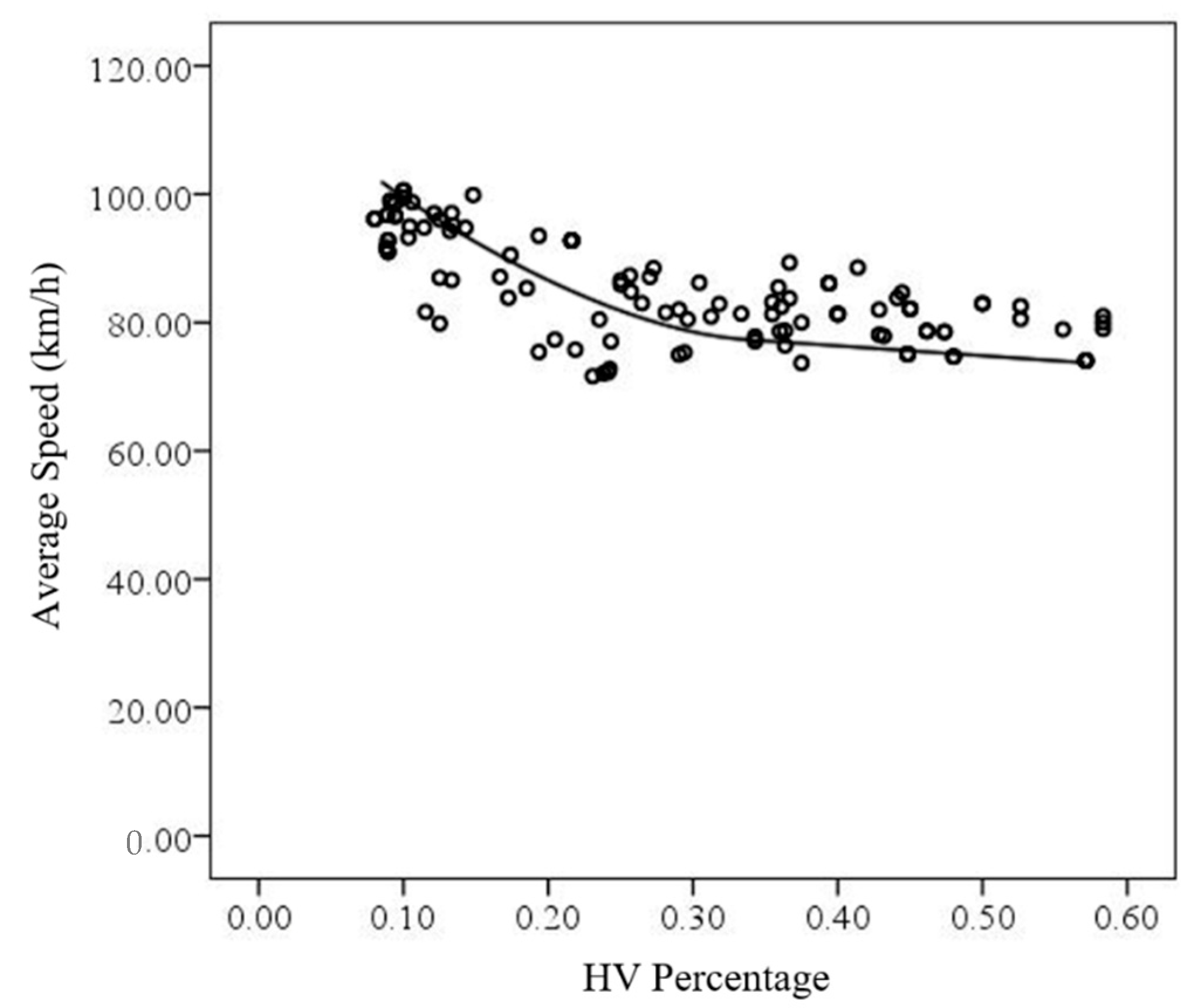
Field data show that the percentage of HVs on the driving lane ranges from 0.08 to 0.58; the scatterplot for HV percentage and average speed is illustrated in Figure 3.

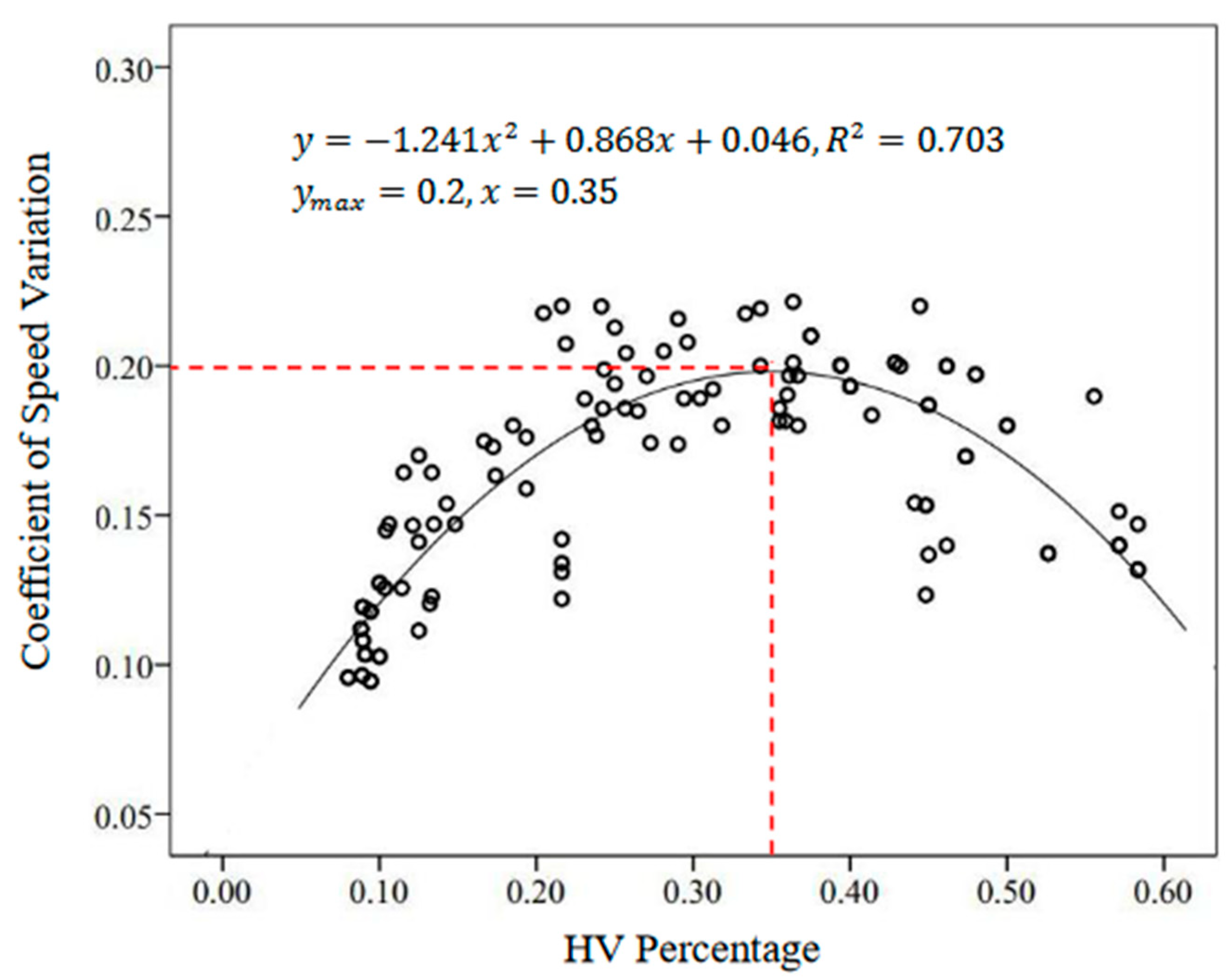
Through Pearson correlation analysis, it was concluded that the correlation coefficient is −0.717 ($p=0.000$), indicating that average speed decreases with HV percentage. This is particularly significant when HV percentage is larger than 30%. In addition, this paper employs the standard deviation of speed as a surrogate measure of speed variation to reveal the impact of HV percentage on speed variation, as illustrated in Figure 4. In general, it was found that the coefficient of speed variation first increases with HV percentage and peaks when HV percentage is at around 0.35. Then, the coefficient of speed variation decreases with HV percentage.

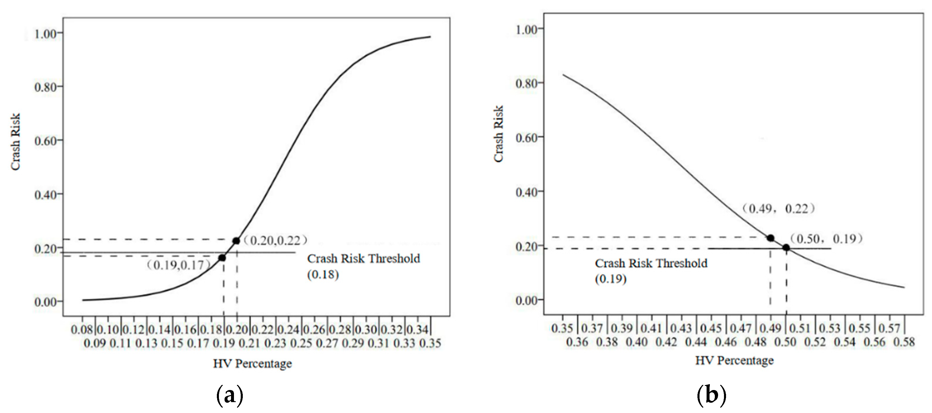
To quantitively assess the crash risk under various HV percentages, this paper employs Binary Logistic Regression Modeling to reveal the impact of HV percentage on speed variation. Two separate models were developed: Model 1 for HV percentage between 0.08 and 0.35; Model 2 for HV percentage between 0.35 and 0.58. For each model, this paper identified a crash risk threshold to differentiate low and high crash risk statuses. The low-crash risk threshold was determined based on the 85th percentile coefficient of speed variation that has been presented in Figure 4 (i.e., Model 1: Speed Variation Coefficient < 0.18; Model 2: Speed Variation Coefficient < 0.19). The Binary Logistic regression modeling was conducted based on the IBM SPSS software package, where low-crash risk status was encoded as “0” and high-crash risk status was encoded as “1”, as specified in

Table 6. Speed Variation Coefficients under Various HV Percentages.

Speed Variation Coefficient for Two Logistic Models		Parameter Encoding	Level of Crash Risk *
Model 1 (0.08 < HV < 0.350	Model 2 (0.35 < HV < 0.58)
Cv$\le$0.18	Cv$\le$0.19	0	Low
Cv > 0.18	Cv > 0.19	1	High

Note: * Low- and High-levels of crash risk refer to low- and high-speed variation coefficients, respectively.

.

Binary Logistic regression modeling results are listed in

Table 7. Binary Logistic Regression Modeling Results.

Binary Model		Regression Coefficient	Standard Deviation	Wald Statistic	Degree of Freedom	Significance *
Model 1 (0.08 < HV < 0.35)	HV%	35.953	8.971	16.060	1	0.000
	Constant	−8.416	2.105	15.979	1	0.000
Model 2 (0.35 < HV < 0.58)	HV%	−20.176	6.455	9.769	1	0.002
	Constant	8.643	2.811	9.453	1	0.002

Note: * 0.05 significance level.

. Results show that both the regression coefficient and the constant term are nonzero parameters, and the modeling results are statistically significant at the 0.05 significance level. Therefore, the probabilities of high-crash risk for the two models could be depicted as follows:

$$P\left(y =1\right)=\{\begin{array}{c}\frac{e^{-8.416+35.953x}}{1+e^{-8.416+35.953x}} \left(0.08\le x\le 0.35\right)\\ \frac{e^{-20.176x+8.643}}{1+e^{-20.176x+8.643}} \left(0.35\le x\le 0.58\right)\end{array}$$

(7)

where:

• $x$ refers to HV percentage;
• $P\left(y =1\right)$ refers to the probabilities of high-crash risk.

Accordingly, the impacts of HV percentage on crash risk are depicted, as illustrated in Figure 5. Results show that, when HV percentage is between 0.19 and 0.5, the variation of speed on a freeway tends to be more significant, which is expected to result in a high risk of rear-end collision. In comparison, when HV percentage is either below 0.19 or exceed 0.5, a low risk of rear-end collision is expected, which is mainly due to the low variation in speed.

4.2. Risk Assessment for Different Vehicle-Following Patterns

In real-world conditions, a rear-end collision is a small-probability event, particularly considering the relatively short field data collection period. Therefore, this paper employs time-to-collision (TTC) and deceleration rate to avoid a crash (DRAC) as surrogate measures of safety for assessing the rear-end crash risk of different vehicle-following patterns. TTCs and DRACs are estimated based on the speed difference and vehicle-following distance of each vehicle-following pair. A lower TTC indicates a higher risk of rear-end collision, and a larger DRAC is related to a higher rear-end collision risk. TTC and DRAC are calculated through Equations (8) and (9), respectively.

$${\mathrm{TTC}}_i = \frac{x_{i-1}\left(t\right)-x_i\left(t\right)-L_{i-1}}{v_i\left(t\right)-v_{i-1}\left(t\right)}, \forall v_i\left(t\right)>v_{i-1}\left(t\right)$$

(8)

where:

• ${\mathrm{TTC}}_i$ refers to the time to collision (sec) between following vehicle ($i$) and leading vehicle ($i-1$);
• $x_{i-1}\left(t\right)$ refers to the location of the leading vehicle at time $t$;
• $x_i\left(t\right)$ refers to the location of the following vehicle at time $t$;
• $v_{i-1}\left(t\right)$ refers to the speed of the leading vehicle (m/s) at time $t$;
• $v_i\left(t\right)$ refers to the speed of the following vehicle (m/s) at time $t$;
• $L_{i-1}$ is the length (m) of the leading vehicle.

$${\mathrm{DRAC}}_i = \frac{\delta v}{\mathsf{∆}t} = \frac{v_i\left(t\right)-v_{i-1}\left(t\right)}{\mathsf{∆}t} = \frac{{\left[v_i\left(t\right)-v_{i-1}\left(t\right)\right]}^2}{x_{i-1}-x_i-L_{i-1}}, \forall v_i\left(t\right)>v_{i-1}\left(t\right)$$

(9)

where:

${\mathrm{DRAC}}_i$ 

refers to the minimum required deceleration rate (m/s²) which a vehicle has to apply to avoid a crash with the leading vehicle;

$\delta v$ 

refers to the speed difference (m/s) between leading vehicle and following vehicle;

$\mathsf{∆}t$ 

refers to TTC.

Based on the extracted speed and vehicle-following distance data for the identified vehicle-following pairs, TTC and DRAC for each vehicle-following pair were calculated and analyzed. The average, median, and the 95th percentile of TTC and DRAC for each vehicle-following pattern, as well as Kolmogorov– Smirnov (K–S) normal distribution test results are presented in

Table 8. Time-to-Collision (TTC) and Deceleration Rate to Avoid a Crash (DRAC) of difference Vehicle-Following Patterns.

Vehicle-Following Pattern	Sample Size	Surrogate Measure of Safety (SMoS)	Average	S.D.	Median	95th Percentile	K–S Test	Significance *
PC-PC	1045	TTC	8.11	4.03	7.49	7.94	0.069	0.000
		DRAC	3.50	8.58	2.09	2.72	0.347	0.000
PC-HV	134	TTC	6.61	4.03	5.91	6.58	0.091	0.009
		DRAC	8.18	17.75	3.63	5.08	0.325	0.000
HV-PC	340	TTC	9.86	4.65	9.22	9.79	0.068	0.001
		DRAC	2.56	2.93	1.66	2.16	0.206	0.000
HV-HV	112	TTC	8.56	5.06	7.75	8.44	0.124	0.000
		DRAC	4.38	6.97	2.23	3.19	0.289	0.000

Note: * 0.05 significance level. K–S test refers to the Kolmogorov–Smirnov test.

.

Results show that, on average, TTC of the PC-HV vehicle-following pattern is the smallest among the four vehicle-following patterns (6.61 s), followed by the PC-PC vehicle-following pattern (8.28 s), the HV-HV vehicle-following pattern (8.80 s), and the HV-PC vehicle-following pattern (9.35 s). In terms of DRAC, it was found that the PC-HV vehicle-following pattern has the highest DRAC among the four vehicle-following patterns (8.18 m/s²), followed by the HV-HV vehicle-following pattern (4.38 m/s²), the PC-PC vehicle-following pattern (3.50 m/s²), and the HV-PC vehicle-following pattern (2.56 m/s²). Both TTC and DRAC results indicate that the PC-HV vehicle-following pattern has the highest risk of rear-end collision, and the HV-PC vehicle-following pattern has the lowest rear-end collision risk. K–S test results indicate that the p-values of TTC and DRAC for all the four vehicle-following patterns are not significant at 0.05 significance level, indicating that the TTC and DRAC of the four vehicle-following patterns are not normally distributed.

5. Safe Vehicle-Following Headways

In reality, the majority of rear-end collisions are attributed to insufficient vehicle-following distance [21,48,49]. Because the braking capability of the two vehicle categories varies, the minimum safe vehicle-following distances for different vehicle-following patterns vary. With this concern, this section aims at determining the minimum safe vehicle-following distances for various vehicle-following patterns based on a micro-level analysis of vehicle braking process.

When a leading vehicle driver slams the brakes on, the minimum safe distance ($D$) for the following vehicle to avoid a rear-end collision is mainly determined by the difference of braking distances of the leading vehicle ($S_l$) and the following vehicle ($S_f$), and the safe stopping distance ($l$) between the two vehicles, as depicted in Equation (10).

$$D = S_f-S_l+l$$

(10)

where:

• $S_f$ refers to the braking distance (m) of the following vehicle starting from the braking process;
• $S_l$ refers to the braking distance (m) of the leading vehicle starting from the braking process;
• $l$ refers to the safe distance (m) between the leading vehicle and the following vehicle.

Generally speaking, a driver’s braking process consists of four steps: (1) driver perception and reaction step, (2) vehicle brake response step, (3) driver braking step, and (4) deceleration step. For the following vehicle, the braking process consists of all these four steps; the time required for performing the four steps are denoted as $t_{f1}$, $t_{f2}$, $t_{f3}$, and $t_{f4}$, respectively. During the driver perception and reaction and the vehicle brake response steps, the speed of the following vehicle is assumed to remain a constant speed that equals its vehicle-following speed ($v_f$); accordingly, the distances traveled during these two steps are $S_{f1}$ and $S_{f2}$, as depicted in Equations (11) and (12), respectively.

$$S_{f1} = {\int }_0^{t_{f1}}{v}_{f1}dt = v_{f1}\times t_{f1}$$

(11)

$$S_{f2} = {\int }_0^{t_{f2}}{v}_{f2}dt = v_{f2}\times t_{f2}$$

(12)

$$S_{f3} = {\int }_0^{t_{f3}}\left(v_{fg}-{\int }_0^t\frac{a_{fmax}\times h}{t_f}dh\right)dt = v_f\times t_{f3}-\frac{1}{6}{a}_f\times t_{f3}^2$$

(13)

$$S_{f4} = \frac{{(v_f-{\int }_0^{v_{f3}}\frac{a_{fmax}\times h}{t_{f3}}dh)}^2}{2\times a_{fmax}} = \frac{v_f{}^2}{ 2\times a_f}+\frac{1}{8}{a}_f\times t_{f3}^2-\frac{1}{2}{v}_f\times t_{f3}$$

(14)

During the driver braking step, the deceleration rate of the following vehicle increases from zero to the vehicle’s maximum deceleration ($a_{fmax}$). To simplify the modeling, this paper assumes that the vehicle deceleration rate increases linearly with time; then, distance traveled during this step ($S_{f3}$) could be described by Equation (13). During the deceleration step, the speed of the following vehicle decreases to zero; distance traveled during this step ($S_{f4}$) is estimated by Equation (14). An illustration of the braking process and distance traveled during each step is presented in Figure 6.

For each vehicle-following pair, driver perception and reaction time and vehicle brake response time will not be taken into account for the leading vehicle. Prior to the braking process, the travel speed of the leading vehicle is denoted as $v_l$. Similarly, during the driver braking step, the deceleration rate of the leading vehicle increases from zero to the maximum vehicle deceleration capability ($a_{lmax}$). Distance traveled during this step ($S_{l3}$) is described by Equation (15). During the deceleration step, the speed of the leading vehicle decreases to zero; distance traveled during this step ($S_{l4}$) could be estimated by Equation (16).

$$S_{l3} = {\int }_0^{t_{l3}}\left(v_l-{\int }_0^t\frac{a_{lmax}\times h}{t_{l3}}dh\right)dt = v_l\times t_{l3}-\frac{1}{6}{a}_{lmax}\times t_{l3}^2$$

(15)

$$S_{l4} = \frac{{(v_l-{\int }_0^{v_{l3}}\frac{a_l\times h}{t_{l3}})}^2}{2\times a_{lmax}} = \frac{v_l{}^2}{2\times a_{lmax}}+\frac{1}{8}{a}_{lmax}\times t_{l3}^2-\frac{1}{2}{v}_l\times t_{l3}$$

(16)

Substituting Equations (11)–(16) to Equation (10), the minimum safety distance could be estimated as follows:

$$D = \left(S_{f1}+S_{f2}+S_{f3}+S_{f4}\right)-\left(S_{l3}+S_{l4}\right)+l$$

(17)

$$\begin{gathered} D = \left[\left(t_{f1}+t_{f2}+\frac{1}{2}{t}_{f3}\right)v_f+\frac{v_f^2}{2\times a_{fmax}}-\frac{1}{24}{a}_{fmax}\times t_{f3}^2\right] \\ -\left(\frac{1}{2}{v}_l\times t_l+\frac{v_l{}^2}{2\times a_{lmax}}-\frac{1}{24}{a}_{lmax}\times t_{l3}^2\right)+l \end{gathered}$$

(18)

Because driver braking time ($t_3$) is usually a small number (i.e., 0.1 s), the impacts of $\frac{1}{24}{a}_l\times t_{l3}^2$ and $\frac{1}{24}{a}_f\times t_{f3}^2$ could be ignored. This paper assumes that $t_{f3} = t_{l3} = t_3$, and $v_l = v_f-\delta v$; then, Equation (18) could be simplified as:

$$D = v_f\left(t_{f1}+t_{f2}\right)+\frac{1}{2}\times t_3\delta v+\frac{v_f^2}{2\times a_{fmax}}-\frac{{\left(v_f-\delta v\right)}^2}{2\times a_{lmax}}+l$$

(19)

Based on the proposed model, minimum safe vehicle-following distance is determined by the following factors: vehicle-following speed ($v_f$), speed difference ($\delta v$), following vehicle driver’s perception time ($t_1$), vehicle brake response time ($t_2$), maximum deceleration rate ($a_{max}$), driver braking time ($t_3$), and safe brake distance ($l$). Specifically, the minimum and maximum vehicle-following speeds were determined as 60 and 120 km/h, which are consistent with the post speed limits of the study site. Based on the descriptive statistics analysis, the absolute speed differences of the collected vehicle-following pairs are within 50 km/h. Because this paper only considers the condition that the following vehicle has a larger speed than the leading vehicle, the speed difference was determined as 0 to 50 km/h. Based on previous research and existing guidelines, the default value for the other parameters are determined as follows: Driver perception and reaction time was determined as 1.6 s, and driver braking time was determined as 0.1 s. Maximum deceleration rates for passenger cars and heavy vehicles were determined as 8.5 and 7.2 m/s², respectively. Safe braking distances for passenger cars and heavy vehicles were determined as 3 and 5 m, respectively. Brake response times for passenger cars and heavy vehicles were determined as 0.175 and 0.6 s, respectively.

Then, the minimum safety vehicle-following distances (i.e., space headways) under various travel speeds and speed differences for each vehicle-following pattern could be estimated as follows:

Passenger Car—Passenger Car:

$$D_{PC-PC} = v\left(1.6+0.175\right)+\frac{1}{2}\times 0.1\delta v+\frac{v^2-{\left(v-\delta v\right)}^2}{2\times 8.5}+3$$

(20)

Passenger Car—Heavy Vehicle:

$$D_{PC-HV} = v\left(1.6+0.6\right)+\frac{1}{2}\times 0.1\delta v+\frac{v^2}{2\times 7.2}-\frac{{\left(v-\delta v\right)}^2}{2\times 8.5}+5$$

(21)

Heavy Vehicle—Passenger Car:

$$D_{HV-PC} = v\left(1.6+0.175\right)+\frac{1}{2}\times 0.1\delta v+\frac{v^2}{2\times 8.5}-\frac{{\left(v-\delta v\right)}^2}{2\times 7.2}+3$$

(22)

Heavy Vehicle—Heavy Vehicle:

$$D_{HV-HV} = v\left(1.6+0.6\right)+\frac{1}{2}\times 0.1\delta v+\frac{v^2-{\left(v-\delta v\right)}^2}{2\times 7.2}+5$$

(23)

Accordingly, the minimum space headways for each vehicle-following pattern are calculated and summarized in

Table 9. Minimum Safe Space Headways for PC-PC Vehicle-Following Patten.

Following Speed (km/h)	Minimum Safe Space Headway (m) under Various Speed Differences (km/h)
	0	5	10	15	20	25	30	35	40	45	50
60	32.6	n/a	n/a	n/a	n/a	n/a	n/a	n/a	n/a	n/a	n/a
65	35.0	38.0	n/a	n/a	n/a	n/a	n/a	n/a	n/a	n/a	n/a
70	37.5	40.6	43.6	n/a	n/a	n/a	n/a	n/a	n/a	n/a	n/a
75	40.0	43.3	46.5	49.4	n/a	n/a	n/a	n/a	n/a	n/a	n/a
80	42.4	46.0	49.4	52.5	55.4	n/a	n/a	n/a	n/a	n/a	n/a
85	44.9	48.7	52.3	55.7	58.8	61.7	n/a	n/a	n/a	n/a	n/a
90	47.4	51.4	55.2	58.8	62.2	65.3	68.2	n/a	n/a	n/a	n/a
95	49.8	54.1	58.1	62.0	65.6	68.9	72.0	75.0	n/a	n/a	n/a
100	52.3	56.8	61.1	65.1	68.9	72.5	75.9	79.0	82.0	n/a	n/a
105	54.8	59.5	64.0	68.2	72.3	76.1	79.7	83.0	86.2	89.1	n/a
110	57.2	62.2	66.9	71.4	75.7	79.7	83.5	87.1	90.5	93.6	96.5
115	59.7	64.9	69.8	74.5	79.0	83.3	87.4	91.2	94.8	98.1	101.2
120	62.2	67.6	72.7	77.7	82.4	86.9	91.2	95.2	99.0	102.6	106.0

,

Table 10. Minimum Safe Space Headways for PC-HV Vehicle-Following Patten.

Following Speed (km/h)	Minimum Safe Space Headway (m) under Various Speed Differences (km/h)
	0	5	10	15	20	25	30	35	40	45	50
60	44.6	n/a	n/a	n/a	n/a	n/a	n/a	n/a	n/a	n/a	n/a
65	48.2	51.1	n/a	n/a	n/a	n/a	n/a	n/a	n/a	n/a	n/a
70	51.8	54.9	57.8	n/a	n/a	n/a	n/a	n/a	n/a	n/a	n/a
75	55.4	58.8	61.9	64.8	n/a	n/a	n/a	n/a	n/a	n/a	n/a
80	59.1	62.7	66.1	69.2	72.1	n/a	n/a	n/a	n/a	n/a	n/a
85	62.9	66.7	70.3	73.6	76.8	79.7	n/a	n/a	n/a	n/a	n/a
90	66.6	70.7	74.5	78.1	81.4	84.6	87.8	n/a	n/a	n/a	n/a
95	70.4	74.7	78.8	82.6	86.2	89.5	92.7	95.6	n/a	n/a	n/a
100	74.3	78.8	83.1	87.1	90.9	94.5	97.9	101.0	103.9	n/a	n/a
105	78.2	82.9	87.4	91.7	95.7	99.5	103.1	106.5	109.6	112.5	n/a
110	82.1	87.1	91.8	96.3	100.6	104.6	108.4	112.0	115.4	118.5	121.4
115	86.1	91.3	96.2	101.0	105.4	109.7	113.8	117.6	121.2	124.5	127.7
120	90.1	95.5	100.7	105.7	110.4	114.9	119.1	123.2	127.0	130.6	133.9

,

Table 11. Minimum Safe Space Headways for HV-PC Vehicle-Following Patten.

Following Speed (km/h)	Minimum Safe Space Headway (m) under Various Speed Differences (km/h)
	0	5	10	15	20	25	30	35	40	45	50
60	29.6	n/a	n/a	n/a	n/a	n/a	n/a	n/a	n/a	n/a	n/a
65	31.6	35.0	n/a	n/a	n/a	n/a	n/a	n/a	n/a	n/a	n/a
70	33.5	37.1	40.6	n/a	n/a	n/a	n/a	n/a	n/a	n/a	n/a
75	35.4	39.3	43.0	46.4	n/a	n/a	n/a	n/a	n/a	n/a	n/a
80	37.2	41.4	45.4	49.1	52.5	n/a	n/a	n/a	n/a	n/a	n/a
85	39.0	43.4	47.	51.6	55.3	58.8	n/a	n/a	n/a	n/a	n/a
90	40.7	45.4	50.0	54.2	58.2	61.8	65.35	n/a	n/a	n/a	n/a
95	42.4	47.5	52.2	56.7	60.9	64.9	68.6	72.0	n/a	n/a	n/a
100	44.1	49.4	54.4	59.2	63.7	67.9	71.9	75.5	79.0	n/a	n/a
105	45.7	51.2	56.6	61.6	66.4	70.9	75.1	79.0	82.7	86.1	n/a
110	47.3	53.1	58.7	64.0	69.0	73.8	78.3	82.5	86.4	90.1	93.6
115	48.9	55.0	60.8	66.4	71.6	76.7	81.4	85.9	90.1	94.1	97.8
120	50.4	56.7	62.9	68.6	74.2	79.5	84.5	89.3	93.8	98.0	102.0

and

Table 12. Minimum Safe Space Headways for HV-HV Vehicle-Following Patten.

Following Speed (km/h)	Minimum Safe Space Headway (m) under Various Speed Differences (km/h)
	0	5	10	15	20	25	30	35	40	45	50
60	41.7	n/a	n/a	n/a	n/a	n/a	n/a	n/a	n/a	n/a	n/a
65	44.7	48.1	n/a	n/a	n/a	n/a	n/a	n/a	n/a	n/a	n/a
70	47.8	51.4	54.9	n/a	n/a	n/a	n/a	n/a	n/a	n/a	n/a
75	50.8	54.8	58.5	61.9	n/a	n/a	n/a	n/a	n/a	n/a	n/a
80	53.9	58.1	62.1	65.8	69.2	n/a	n/a	n/a	n/a	n/a	n/a
85	56.9	61.4	65.6	69.6	73.3	76.7	n/a	n/a	n/a	n/a	n/a
90	60	64.8	69.2	73.5	77.4	81.1	84.5	n/a	n/a	n/a	n/a
95	63.1	68.1	72.8	77.3	81.6	85.5	89.2	92.6	n/a	n/a	n/a
100	66.1	71.4	76.4	81.2	85.7	89.9	93.9	97.5	102.0	n/a	n/a
105	69.2	74.7	80.0	85.0	89.8	94.3	98.5	102.5	106.3	109.6	n/a
110	72.2	78.1	83.6	88.9	93.9	98.7	103.2	107.4	111.3	115.0	118.5
115	75.3	81.4	87.2	92.8	98.1	103.1	107.8	112.3	116.6	120.5	124.3
120	78.3	84.7	90.8	96.6	102.1	107.5	112.5	117.3	121.8	126.0	129.9

.

Results show that, with the increase of vehicle-following speed and/or speed differences, the minimum safe following distances indicate an increasing trend for all four vehicle-following patterns. Under an identical vehicle-following speed and speed difference, it was found that the PC-HV vehicle-following pattern requires the largest minimum safe space headway, followed by the HV-HV, PC-PC, and HV-PC vehicle-following patterns, respectively. This also suggests that the PC-HV vehicle-following pattern poses the highest crash risk in comparison with other vehicle-following patterns.

6. Concluding Remarks

This paper employed a video-based speed data collection approach to investigate the impacts of heavy vehicles on speed variation; ultimately, it assessed the risk of rear-end crashes for different vehicle-following patterns. Field data revealed that average speed displays a decreasing trend with the increase of HV percentage; nevertheless, the variation of speed first increases with HV percentage and reaches the maximum when HV percentage is at around 0.35; then, it shows a decreasing trend with HV percentage. Based on a binary logistic regression modeling of the collected speed data, this paper concluded that a high risk of rear-end collision is expected when HV percentage is between 0.19 and 0.5. In comparison, when HV percentage is either below 0.19 or beyond 0.5, a low risk of rear-end collision is anticipated.

Then, this paper employed TTC and DRAC as surrogate measures of safety to assess the crash risk of four vehicle-following patterns. Results show that the PC-HV vehicle-following pattern has the lowest TTC and the highest DRAC (i.e., the highest risk of rear-end collision), and the HV-PC vehicle-following pattern has the highest TTC and lowest DRAC (i.e., the lowest rear-end collision risk). In addition, based on the analytical modeling of the vehicle braking process, this paper develops models for estimating the minimum safe vehicle-following distances for each vehicle-following pattern under various travel speeds and speed differences. In general, it was concluded that, for a given travel speed and speed difference scenario, HVs require a larger safe following distance than PCs. Specifically, the PC-HV vehicle-following pattern requires the largest minimum safe space headway, following by the HV-HV, PC-PC, and HV-PC vehicle-following patterns.

In summary, findings from this research reveal that there are diversities in the minimum safe vehicle-following distance for different vehicle-following patterns, indicating that the crash risks of different vehicle-following patterns vary. This presents some preliminary insights to transportation engineers in terms of the development of crash mitigation strategies such as HV access and lane use management, variable speed limits, and driver’s safety education on the selection of following headways, etc. In addition, with the increasing popularity of connected vehicle (CV) technology, the estimated minimum safe vehicle-following headways also present potentials to advance the development of real-time in-vehicle forward collision warnings to minimize the risk of rear-end crash.

Nevertheless, it is necessary to point out that the traffic flow data used by this research were collected from one representative freeway segment under normal weather condition, and crash risks were assessed solely based on vehicles’ speed, vehicle-following headways, and default driver behavior and vehicle dynamics performances. In practice, vehicle-following behavior under different demand levels might vary and tends to be affected by a wider range of factors such as roadway geometry configurations, driver demographical features, post speed limits, and weather conditions, etc. For instance, drivers usually keep a larger following distance under adverse weather conditions (e.g., rainy, foggy, snowy, windy weather) than under normal weather condition, and the changes in driving behavior will affect the safety performance assessment results. Therefore, further works should further investigate the impacts of these various factors on the safety performance of various vehicle-following patterns. The presented video-based data collection and extraction procedure could be used for similar research activities if the adverse weather event does not significantly impact the visibility of vehicles and pavement markings. In cases where the research site is under severe weather conditions such as heavy rain, dense fog, heavy snow, etc., this paper recommends using calibrated machine vision or machine learning technologies to process the capture videos to extract the vehicle-following headways.

References

- Xu, C.; Wang, Y.; Liu, P.; Wang, W.; Bao, J. Quantitative risk assessment of freeway crash casualty using high-resolution traffic data. Reliab. Eng. Syst. Saf. 2018, 169, 299–311. [Google Scholar] [CrossRef]
- Zhang, J.; Wang, Y.; Lu, G. Impact of heterogeneity of car-following behavior on rear-end crash risk. Accid. Anal. Prev. 2019, 125, 275–289. [Google Scholar] [CrossRef]
- Mahmud, S.M.; Ferreira, L.; Hoque, S.; Tavassoli, A. Micro-level safety risk assessment model for a two-lane heterogeneous traffic environment in a developing country: A comparative crash probability modeling approach. J. Saf. Res. 2019, 69, 125–134. [Google Scholar] [CrossRef]
- Yin, W.; Zhang, Y. Identification Method for Optimal Urban Bus Corridor Location. Sustainability 2020, 12, 7167. [Google Scholar] [CrossRef]
- Lin, C.; Wang, K.; Wu, D.; Gong, B. Passenger Flow Prediction Based on Land Use around Metro Stations: A Case Study. Sustainability 2020, 12, 6844. [Google Scholar] [CrossRef]
- Dulebenets, M.A.; Kavoosi, M.; Abioye, O.; Pasha, J. A self-adaptive evolutionary algorithm for the berth scheduling problem: Towards efficient parameter control. Algorithms 2018, 11, 100. [Google Scholar] [CrossRef] [Green Version]
- Abioye, O.F.; Dulebenets, M.A.; Pasha, J.; Kavoosi, M. A vessel schedule recovery problem at the liner shipping route with emission control areas. Energies 2019, 12, 2380. [Google Scholar] [CrossRef] [Green Version]
- Ventura, R.V.; Cabo, M.; Caixeta, R.; Fernandes, E.; Aprigliano Fernandes, V. Air Transportation Income and Price Elasticities in Remote Areas: The Case of the Brazilian Amazon Region. Sustainability 2020, 12, 6039. [Google Scholar] [CrossRef]
- Blower, D. The Relative Contribution of Truck Drivers and Passenger Vehicle Drivers to Truck-Passenger Vehicle Traffic Crashes; Michigan Report Number: UMTRI-98-25; The University of Michigan Transportation Research Institute: Ann Arbor, MI, USA, 1998. [Google Scholar]
- Golob, T.F.; Recker, W.W.; Alvarez, V.M. Freeway safety as a function of traffic flow. Accid. Anal. Prev. 2004, 36, 933–946. [Google Scholar] [CrossRef]
- Hossain, M.; Muromachi, Y. Understanding crash mechanism on urban expressways using high-resolution traffic data. Accid. Anal. Prev. 2013, 57, 17–29. [Google Scholar] [CrossRef]
- Wang, C.; Quddus, M.; Ison, S.G. The effect of traffic and road characteristics on road safety: A review and future research direction. Saf. Sci. 2013, 57, 264–275. [Google Scholar] [CrossRef]
- Roshandel, S.; Zheng, Z.; Washington, S. Impact of real-time traffic characteristics on freeway crash occurrence: Systematic review and meta-analysis. Accid. Anal. Prev. 2015, 79, 198–211. [Google Scholar] [CrossRef]
- van Beinum, A.; Farah, H.; Wegman, F.; Hoogendoorn, S. Critical Assessment of Methodologies for Operations and Safety Evaluations of Freeway Turbulence. Transp. Res. Rec. 2016, 2556, 39–48. [Google Scholar] [CrossRef] [Green Version]
- Zhang, G.; Wang, Y.; Wei, H.; Chen, Y. Examining Headway Distribution Models with Urban Freeway Loop Event Data. Transp. Res. Rec. 2007, 1999, 141–149. [Google Scholar] [CrossRef]
- Loulizi, A.; Bichiou, Y.; Rakha, H. Steady-State Car-Following Time Gaps: An Empirical Study Using Naturalistic Driving Data. J. Adv. Transp. 2019, 2019, 7659496. [Google Scholar] [CrossRef] [Green Version]
- Wasielewski, P. The Effect of Car Size on Headways in Freely Flowing Freeway Traffic. Transp. Sci. 1979, 15, 364–378. [Google Scholar] [CrossRef]
- Kerner, B.S.; Klenov, S.L. Special-temporal patterns in heterogeneous traffic flow with a variety of driver behavioural characteristics and vehicle parameters. J. Phys. A Math. Gen. 2004, 37, 8753–8788. [Google Scholar] [CrossRef]
- Ossen, S.; Hoogendoorn, S.P. Heterogeneity in car-following behavior: Theory and empirics. Transp. Res. Part C 2011, 19, 182–195. [Google Scholar] [CrossRef]
- Weng, J.; Meng, Q.; Yan, X. Analysis of work zone rear-end crash risk for different vehicle-following patterns. Accid. Anal. Prev. 2014, 72, 449–457. [Google Scholar] [CrossRef]
- Dimitriou, L.; Stylianou, K.; Abdel-Aty, M.A. Assessing rear-end crash potential in urban locations based on vehicle-by-vehicle interactions, geometric characteristics and operational conditions. Accid. Anal. Prev. 2018, 118, 221–235. [Google Scholar] [CrossRef]
- Geng, X.; Liang, H.; Xu, H.; Yu, B. Influence of Leading-Vehicle Types and Environmental Conditions on Car-Following Behavior. IFAC PapersOnLine 2016, 49, 151–156. [Google Scholar] [CrossRef]
- Kim, S.K.; Song, T.J.; Rouphail, N.M.; Aghdashi, S.; Amaro, A.; Gonçalves, G. Exploring the association of rear-end crash propensity and micro-scale driver behavior. Saf. Sci. 2016, 89, 45–54. [Google Scholar] [CrossRef]
- Durrani, U.; Lee, C.; Maoh, H. Calibrating the Wiedemann’s vehicle-following model using mixed vehicle-pair interactions. Transp. Res. Part C 2016, 67, 227–242. [Google Scholar] [CrossRef]
- Hamzeie, R.; Savolaninen, P.T.; Gates, T.J. Driver speed selection and crash risk: Insights from the naturalistic driving study. J. Saf. Res. 2017, 63, 187–194. [Google Scholar] [CrossRef] [PubMed]
- Xiong, X.; Wang, M.; Cai, Y.; Chen, L.; Farah, H.; Hagenzieker, M. A forward collision avoidance algorithm based on driver braking behavior. Accid. Anal. Prev. 2019, 129, 30–43. [Google Scholar] [CrossRef] [PubMed] [Green Version]
- Quddus, M. Exploring the Relationship between Average Speed, Speed Variation, and Accident Rates Using Spatial Statistical Models and GIS. J. Transp. Saf. Secur. 2013, 5, 27–45. [Google Scholar] [CrossRef]
- FHWA. Human Factor Issues in Intersection Safety; Report No. FHWA-SA-10-005; U.S. Department of Transportation: Washington, DC, USA, 2009.
- Ye, F.; Zhang, Y. Vehicle Type-Specific Headway Analysis Using Freeway Traffic Data. Transp. Res. Rec. 2009, 2124, 222–230. [Google Scholar] [CrossRef]
- Aghabayk, K.; Sarvi, M.; Young, W. Including heavy vehicles in a car-following model: Modelling, calibrating and validating. J. Adv. Transp. 2016, 50, 1432–1446. [Google Scholar] [CrossRef]
- Oh, C.; Park, S.; Ritchie, S.G. A method for identifying rear-end collision risks using inductive loop detectors. Accid. Anal. Prev. 2006, 38, 295–301. [Google Scholar] [CrossRef]
- Abdel-Aty, M.; Pande, A.; Lee, C.; Gayah, V.; Santos, C.D. Crash Risk Assessment Using Intelligent Transportation Systems Data and Real-Time Intervention Strategies to Improve Safety on Freeways. J. Intell. Transp. Syst. 2007, 11, 107–120. [Google Scholar] [CrossRef]
- Shew, C.; Pande, A.; Nuworsoo, C. Transferability and robustness of real-time freeway crash risk assessment. J. Saf. Res. 2013, 46, 80–93. [Google Scholar] [CrossRef] [PubMed] [Green Version]
- Yu, R.; Abdel-Aty, M. Utilizing support vector machine in real-time crash risk evaluation. Accid. Anal. Prev. 2013, 51, 252–259. [Google Scholar] [CrossRef] [PubMed]
- Lao, Y.; Zhang, G.; Wang, Y.; Milton, J. Generalized nonlinear models for rear-end crash risk analysis. Accid. Anal. Prev. 2014, 62, 9–16. [Google Scholar] [CrossRef]
- Kwak, H.C.; Kho, S. Predicting crash risk and identifying crash precursors on Korean expressways using loop detector data. Accid. Anal. Prev. 2016, 88, 9–19. [Google Scholar] [CrossRef] [PubMed]
- Yu, R.; Wang, X.; Yang, K.; Abel-Aty, M. Crash risk analysis for Shanghai urban expressways: A Bayesian semi-parametric modeling approach. Accid. Anal. Prev. 2016, 95, 495–502. [Google Scholar] [CrossRef] [Green Version]
- Mullakkal-Babu, F.A.; Wang, M.; Farah, H.; van Arem, B.; Happee, R. Comparative Assessment of Safety Indicators for Vehicle Trajectories on Highways. Transp. Res. Rec. 2017, 2659, 127–136. [Google Scholar] [CrossRef]
- Hyun, K.; Jeong, K.; Tok, A.; Ritchie, S.G. Assessing crash risk considering vehicle interactions with trucks using point detector data. Accid. Anal. Prev. 2018. [Google Scholar] [CrossRef]
- Zhao, P.; Lee, C. Assessing rear-end collision risk of cars and heavy vehicles on freeways using a surrogate safety. Accid. Anal. Prev. 2018, 113, 149–158. [Google Scholar] [CrossRef] [PubMed]
- Choudhary, P.; Imprialou, M.; Velaga, N.R.; Choudhary, A. Impacts of speed variations on freeway crashes by severity and vehicle type. Accid. Anal. Prev. 2018, 121, 213–222. [Google Scholar] [CrossRef] [Green Version]
- TMRI. Safety Specifications for Power-Driven Vehicles Operating on Roads; Publication No. GB 7258-2012; Traffic Management Research Institute of the Ministry of Public Security (TMRI): Beijing, China, 2012. [Google Scholar]
- Yang, G.; Xu, H.; Tian, Z.; Wang, Z. Vehicle speed and acceleration profile study for metered on-ramps in California. J. Transp. Eng. 2016, 142. [Google Scholar] [CrossRef]
- Gazis, D.C.; Herman, R.; Rothery, R.W. Nonlinear Follow-the-Leader Models for Traffic Flow. Oper. Res. 1961, 9, 545–567. [Google Scholar] [CrossRef]
- Gerlough, D.L.; Huber, M.J. Traffic Flow Theory: A Monograph; Special Report 165; Transportation Research Board: Washington, DC, USA, 1975.
- He, M. Study on Traffic Car-Following Model. Master’s Thesis, Beijing University of Technology, Beijing, China, 2000. (In Chinese). [Google Scholar]
- Wang, D. Traffic Flow Theory; China Communication Press Co., Ltd.: Beijing, China, 2002. (In Chinese) [Google Scholar]
- Michael, P.G.; Leeming, F.C.; Dwyer, W.O. Headway on urban streets: Observational data and an intervention to decrease tailgating. Transp. Res. Part F 2000, 3, 55–64. [Google Scholar] [CrossRef]
- Tanishita, M.; van Wee, B. Impact of vehicle speeds and changes in mean speeds on per vehicle-kilometer traffic accident rates in Japan. IATSS Res. 2017, 41, 107–112. [Google Scholar] [CrossRef] [Green Version]
Figure 1.
Illustration of data collection location and method.
Figure 2.
Illustration of the proposed video-based traffic data extraction approach.
Figure 3.
Scatterplot of the Relationship between Average Speed and HV Percentage.
Figure 4.
Scatterplot of HV Percentage and Coefficient of Speed Variation.
Figure 5.
Relationship between Crash Risk and HV Percentage: (a) 0.08 < HV Percentage < 0.35; (b) 0.35 < HV Percentage < 0.58.
Figure 6.
Graphic illustration of Vehicle Braking Process: (a) Deceleration versus time profile; (b) Braking distance versus time profile.