A Prediction Method of GHG Emissions for Urban Road Transportation Planning and Its Applications


1
School of Transportation, Southeast University, Nanjing 211189, China
2
Department of Civil and Environmental Engineering, University of Wisconsin-Madison, Madison, WI 53706, USA
*
Author to whom correspondence should be addressed.
Sustainability 2020, 12(24), 10251; https://0-doi-org.brum.beds.ac.uk/10.3390/su122410251
Submission received: 17 November 2020
/
Revised: 2 December 2020
/
Accepted: 3 December 2020
/
Published: 8 December 2020
(This article belongs to the Section Sustainable Urban and Rural Development)
Abstract
:The increasing vehicle usage has brought about a sharp increase in greenhouse gas (GHG) emissions of vehicles, which brings severe challenges to the sustainable development of road transportation in Chinese counties. Low-carbon transportation planning is an essential strategy for carbon control from the source of carbon emissions and is crucial to the full transition to a low-carbon future. For transportation planning designers, a quick and accurate estimation of carbon emissions under different transportation planning schemes is a prerequisite to determine the optimal low-carbon transportation development plan. To address this issue, a novel prediction method of hourly GHG emissions over the urban roads network was constructed in this paper. A case study was conducted in Changxing county, and the results indicate the effectiveness of our proposed method. Furthermore, we applied the same approach to 30 other counties in China to analyze the influencing factors of emissions from urban road networks in Chinese counties. The analysis results indicate that the urban road mileage and arterial road ratio are the two most important factors affecting road network GHG emissions in road traffic planning process. Moreover, the method was employed to derive peak hour emission coefficients that can be used to quickly estimate daily or annual GHG emissions. The peak hour emission of CO2, CH4, and N2O accounts for approximately 9–10%, 8.5–10.5%, 5.5–7.5% of daily emissions, respectively. It is expected that the findings from this study would be helpful for establishing effective carbon control strategies in the transportation planning stage to reduce road traffic GHG emissions in counties.
1. Introduction
In 2015, 17 Sustainable Development Goals (SDGs) were adopted by 193 countries for sustainable development over the coming years. All countries are working to develop some policies to achieve equitable compliance with the SDGs at global level in 2030 [1]. Each organization evaluates the SDGs to accurately assess the relative priority of each of the 17 SDGs to its core organizational objectives [2]. Climate action is always identified as a priority SDG to achieve sustainable development [3]. In the whole world, reducing carbon emissions in the transportation sector is always a “core objective” to fight against climate change. How to effectively control traffic negative externalities has always been a research hotspot.
As an essential part of urban traffic, road traffic undertakes the vast majority of traffic travel tasks. It plays an important role in alleviating urban traffic pressure and improving citizens’ travel environment. The increasing vehicle usage has brought about a sharp increase in greenhouse gas (GHG) emissions of vehicles, which curbs the low-carbon transportation development in China. Road traffic has become a key area for energy-saving and pollutant reduction in China. According to the IEA statistics of the International Energy Agency in 2019 [4], China’s total carbon emissions in the past two years have exceeded 10 billion tons, of which the emissions in the transportation sector have reached about 10 percent of China’s total emissions or 1 billion tons. Most of the emissions from the transportation sector were attributed to road transport with approximately 80 percent of all emissions and a total of 800 billion tons. The carbon emissions of road traffic have seriously exceeded the self-purification capacity of the natural environment. As a highly concentrated place for residents to produce and live, the destruction of the ecological environment will undoubtedly cause serious harm to the physical, psychological, and life of urban residents. One of the requirements to consider the future paradigm of green and smart cities should be the reduction of emissions coming from transport [5,6]. The current rate of progress in China is insufficient to achieve equitable compliance with the SDGs at national-level in 2030. Therefore, how to achieve sustainable development of road transportation (low-carbon road transportation) has become a considerable challenge for transportation planning designers [7,8].
The development path of low-carbon road transportation falls into three categories: optimizing the road traffic structure (e.g., road network optimization [9], travel structure optimization [10]), improving energy-saving technologies (e.g., alternative fuels [11], engine improvement [12]), and formulating mandatory policies (e.g., vehicle limit [13], congestion charge [14,15]). Among them, the structural adjustment path is a crucial emission reduction strategy to control from the source of carbon emissions. It aims to break through the bottleneck of traditional vehicle energy-saving technical emission reduction strategies and is an indispensable part of the current development of low-carbon road transportation. Transportation planning has a long-term and structural role in urban development. Once the physical environment of transportation is established, it is tough to adjust the additional emissions from road transportation caused by the unreasonable configuration and layout of transportation facilities [16]. Low-carbon road transportation planning refers to the adjustment and optimization of the planning scheme in consideration of the development needs of low-carbon road transportation during the preparation of the road transportation planning scheme, and the formulation of a carbon control strategy [17]. Its purpose is to reduce road traffic carbon emissions by curbing unreasonable traffic demand. Therefore, low-carbon road transportation planning is the primary technical path to achieve structural adjustment emission reduction.
One essential auxiliary decision-making information for transportation planning designers is the GHG emissions of different planning schemes. They often rely on the emission estimation results to compare different planning options and thus develop effective control measures from the perspective of low-carbon development. To this end, this paper focuses on the research and application of GHG emission estimation for low-carbon road transportation planning, which can lay the foundation for the implementation of low-carbon strategies and is a critical technology to achieve structural emission reduction.
Traditional GHG emissions from vehicles estimation methods fall into two categories, an energy consumption-based method, and a traffic activity data-based method. The energy consumption-based method was first proposed in the Intergovernmental Panel on Climate Change (IPCC) guidelines [18]. The total fuel consumption is multiplied by the fuel carbon emission factor to calculate the carbon emissions. This method requires detailed information on the types of fuel consumed by various modes of transportation and their consumption data, which cannot capture the impact of temporal and spatial characteristics of traffic flow on carbon emissions. It is only for macroscopic estimation of the carbon emissions level of an entire region [19,20,21]. Therefore, this approach is not suitable for the low-carbon assessment of road traffic planning schemes and the identification of emission hotspots. Concerning the traffic activity data-based method, the total emissions are generally obtained by accumulating the product of vehicle kilometers travel (VKT) at various speeds and its corresponding emission rate. Getting and predicting detailed traffic activity parameters is the focus and difficulty of this method. It should be noted that the traffic activity data are divided into static and dynamic data. The static data (e.g., vehicle ownership [22], average VKT of each vehicle type [23,24]) are macroscopic data of traffic flow, which also lack the capability of capturing the impact of traffic flow characteristics on carbon emissions. On the contrary, dynamic traffic activity data (e.g., hourly traffic volume, link-level vehicle speed distribution) can be used to derive hourly and link-level emissions. Liu et al. [25] established the carbon emission inventory of Foshan city by the video data of 198 intersection points in Foshan and the emission factors of the Computer Programme to calculate Emissions from Road Transport (COPERT) IV model. Kholod et al. [26] used traffic survey video data to obtain the average daily traffic volume of each vehicle type on each road type, and then multiplied by the length of each road type to obtain the average daily vehicle kilometers of the entire road network. However, all previous research focuses on the current traffic activity data, and there is no concern about the estimation or prediction of dynamic traffic activity data under the future transportation planning scheme. In addition, detailed dynamic data are almost difficult to obtain as mentioned in previous research. Thus, dynamic traffic activity data estimation or prediction based on one specific transportation planning scheme has become a huge challenge for us.
On the other hand, substantial research has been conducted to study carbon emission and its driving factors at the national, provincial, or city level [27,28,29,30]. So far, it seems that limited research focuses on road traffic carbon emission at county level. Due to the lack of a local-specific emission rates database and related research at county level, road traffic carbon emissions were estimated as the downscale of cities’ carbon emission inventory by economic or population data. How to achieve practical evaluation in the case where county-level data are challenging to obtain is even more of a problem.
Therefore, to better manage traffic emissions in Chinese counties and provide support for sustainable transportation system development, we developed a GHG estimation method for one specific transportation plan based on its indicators in this study. The methodology is not only applicable to the prediction of the GHG emissions from road traffic in planning year but also suitable for the evaluation of carbon emissions of existing road network if current road network indicator data are available. This method is new to the field of GHG emissions prediction from road transportation and helped in identifying key factors and their changes to influence the sustainability of road transportation in any Chinese county. It is a critical technology to achieve structural emission reduction. The main contribution of this study lies in applying only urban road planning indicators to evaluate GHG emissions in the planning year that could be potentially employed by transportation planners or government policy-makers to implement effective carbon control measures and promote low-carbon transportation development.
2. Methodology
2.1. Research Domain, Object, and Framework
A county, one of the administrative divisions in China, is under the jurisdiction of prefecture-level cities, or directly under the authority of a province. It is the most basic administrative unit in China, of which there are a total of 2800. The research domain in this study focuses on the urban roads network of counties in China. Changxing county, one of the largest and most developed counties in Yangtze River Delta, was selected as the representative county for the case study, and we applied the emission prediction method to 30 other counties.
Vehicle emissions are usually produced in multiple processes, such as the start process, running process, and extended idle process, of which running emissions account for the vast majority. Thus, in this study, we focus on the running emissions produced by vehicles.
Regarding the vehicle category, light-duty passenger vehicle (LDPV), light-duty truck (LDT), and motorcycle (MC) accounts for approximately 95–98% of road-users in Chinese counties, according to the vehicle registration data in some counties. With consideration of data acquisition difficulty and accuracy requirements of emissions estimation for transportation planning designers, only the emissions emitted by LDPVs, LDTs, and MCs are considered in this paper. Moreover, in these three types of vehicles, almost all vehicles are powered by gasoline in Chinese counties. Therefore, only gasoline LDPVs, LDTs, and MCs are discussed in the following sections. Table 1 represents the definition of vehicle categories in this study.
Generally, the calculation method of carbon emissions during the road traffic operation process is to collect vehicle emission rates and related motor vehicle activity data. To more accurately assess the GHG emissions with different road types, a road type-based and hourly emission calculation method were adopted in this study, as shown in Equation (1). Based on this, we can derive the daily or annual GHG emissions by summing the carbon emissions per hour.
where represents the emissions (in g/h) of pollutant (CO2, CH4, N2O) during hour ; indicates the emissions of pollutant emitted by vehicle category on the -type road during hour under the speed ; (in veh/h) represents the traffic volume of vehicle category on the -type road at hour under the speed ; represents the length of the -type road (in km); and (in g/km) is the emission rates of pollutant emitted by vehicle category on the -type road during hour under the speed (in km/h).
The emission rates are derived from the local-specific calibration of Motor Vehicle Emission Simulator (MOVES) [31]. Note that the vehicle category adopted in this study is also based on the official vehicle category definition rules adopted by MOVES.
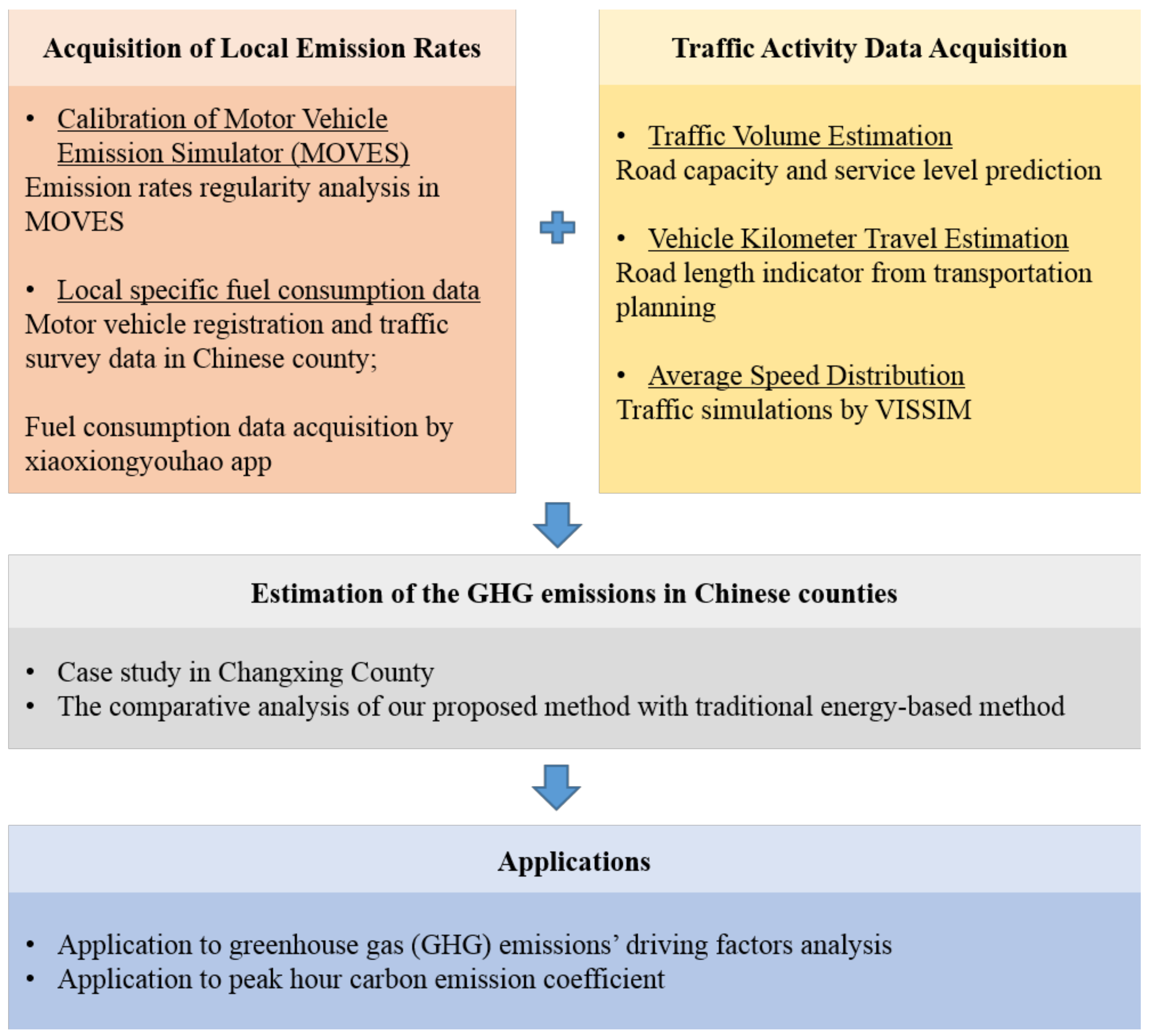
From Equation (1), it was found that the emission rates are the core basis for calculating GHG emissions, and the traffic activity data is another critical parameter. Therefore, the acquisition of emission rates was firstly presented in Section 2.2, and the methods of obtaining and predicting traffic activity data were discussed in Section 2.3. Based on the methodology in Section 2, a case study in Changxing county was conducted in Section 3. Finally, we expand its application on other traffic issues, including the GHG emissions driving factors analysis and the calculation of peak hour emissions coefficient, which were presented in Section 4. Figure 1 illustrates the logical framework of the methodology and its applications in this paper.
2.2. Calibration of MOVES
MOVES, developed by the U.S Environmental Protection Agency (EPA), is a large-scale regulatory traffic emission model in the U.S. (except California). It can estimate road traffic emissions under a variety of scenarios, from macro to micro levels. At present, the MOVES model has developed into one of the most widely used emission calculation models in the world because of its friendly interface and increased customization for international applications. However, MOVES is constructed according to the local traffic conditions in the U.S., so it needs to be calibrated in advance for application in other countries to curb large estimation errors.
The GHG emissions discussed in this paper include carbon dioxide (CO2), methane (CH4), and nitrous oxide (N2O). It is well known that CO2 contributes the most to GHG emissions, the CH4 and N2O emissions are negligible compared to CO2 (approximately one in the thousand). With a comprehensive consideration of the calibration necessity and the workload, we chose to calibrate only CO2 emission rates in this study. For CH4 and N2O, we directly applied the emission rates database embedded in MOVES.
According to the principle of carbon balance (chemical principles), the fuel consumption of vehicles is closely related to its CO2 emissions [32]. The amount of CO2 produced by the fuel is related to the carbon content and the density of the fuel used, as shown in Equation (2).
where is average CO2 emission factor (g/km) vehicle type powered by gasoline and produced in year ; is the average fuel consumption (L/100 km) for vehicle type powered by gasoline and produced in year ; is the density of gasoline; and is the carbon mass fraction of gasoline.
The CO2 emission rates embedded in MOVES generally vary with vehicle speed, model year, temperature (months and hours), vehicle type, and road type. To explore the changing regularity of CO2 emission rates with vehicle speed and model year, we fixed the vehicle type and road type, and then averaged the emission rates at all temperatures in a year. After our exploration of the regularity of MOVES emission rates, it was found that for the different model years, the absolute value of the emission rates under different speed is always unchanged; this relative changing regularity was called speed correction factors (SCF).
Based on the speed correction functions, we can directly develop the local-specific CO2 emission rates model for LDPVs, LDTs, and MCs using the local-specific fuel consumption data, as Equation (3) following.
where is the average CO2 emission factor (g/km) for local vehicle type powered by gasoline and produced in year under an average speed of (km/h); is average CO2 emission factor (g/km) for local vehicle type powered by gasoline and produced in year , which can be derived by Equation (2) based on local real-world average fuel consumption data; and denotes the speed correction function for an average speed of (km/h).
We calculated the average fuel consumption data by model from Xiaoxiongyouhao app and finally got the following data in Table 2.
2.3. Estimation of Traffic Activity Data
The traffic activity data are of significant importance for calculating carbon emissions, and their accuracy directly affect the accuracy of carbon emissions estimation, as described in Section 2.1. Therefore, this subsection mainly describes the acquisition and estimation methods of traffic activity data, including traffic volume, VKT, and average speed distribution.
2.3.1. Hourly Traffic Volume Estimation
It is not always possible to completely derive the actual traffic volume analytically on different road types and during the different time periods under a given transportation planning scheme. In most cases, it is estimated by traffic simulation software (e.g., TransCAD, Paramics). However, it is only applicable to the situation with detailed origin and destination (OD) and road network data. Obtaining OD data is extremely complicated work and also usually produces large errors than the actual travel demand. Therefore, we attempted to explore an alternative method for estimating hourly traffic volume based on road capacity and transportation planning indicators.
Road capacity is divided into basic traffic capacity (or theoretical capacity), possible traffic capacity, and design traffic capacity. The possible capacity refers to the capacity that takes into account the impact of actual road conditions and traffic conditions, which can be derived from the correction of basic capacity, as shown in Equation (4).
where represents the one-way possible traffic capacity on a certain road section, usually expressed in passenger car unit (pcu) per hour per lane. is the basic capacity of a lane, usually we adopt the recommended values of “Urban Road Design Specifications (CJJ 36–90)” according to different road speeds. denotes the correction factor of multiple-lane, which is used to describe the influence on adjacent lane capacity when overtaking of vehicles in the same direction is performed in the case of multiple lanes. is the correction factor of lane width, the width of the lane has a great influence on the driving speed, which in turn affects the road capacity. is the correction factor of mixed environ ment. represents the correction factor of intersections, which mainly depends on the intersection control method and intersection spacing. When the intersection spacing is small, the parking delay at the intersection accounts for a large proportion of the vehicle travel time, which is not conducive to the utilization of road space. represents the correction factor of streetization, buildings on both sides of the road often cause interference from pedestrians and non-motorized vehicles to the car, thereby forcing the car to slow down and reduce road capacity. Finally, is the correction factor of roadside parking. Roadside parking will result in a reduction in the road width and a reduction in lateral clearance. At the same time, the traffic flow will be interfered when a vehicle enters and exits the parking space, which will change the road capacity.
Unlike big cities in China, urban road traffic in counties has its own characteristics. For example, in counties, the lane width is basically less than standard (3.5 m), and the phenomenon of mixed environment of motor vehicle and non-motor vehicle is particularly serious, no matter which type of road. Additionally, due to the improvement of the living standards of the people in the county towns in recent years, vehicle ownership and usage frequency has increased sharply, but the backward parking lot planning has been unable to meet the daily parking demand. Therefore, in the counties of China, the roadside parking phenomenon is particularly serious and is especially obvious on the local roads. The value of the capacity correction coefficient adopted in this paper is shown in Table 3, referring to some empirical values in “Urban Road Design Specifications (CJJ 36–90)” [33]. Note that corresponding changes could be conducted according to the actual situation of their own roads in each county.
It should be noted that the theoretical or possible capacity indicates the maximum traffic flow per unit time passing any selected point on the road using all available lanes. It speaks of how much traffic a road can accommodate. For a given road, its possible traffic capacity should be a fixed value, but actual hourly traffic flow will be different, which will result in different GHG emissions at different times of the day. Level of service (LOS) is related to the capacity, which characterizes how good the operational status of the traffic flow is. For urban roads, the most important indicator to measure the LOS is the saturation of the road section (V/C, namely volume to capacity ratio). Therefore, in this study, we adopted the term “V/C” to derive the actual flow at each time period on a given road. For convenience, three typical time periods of the day are considered and are peak, off-peak, and free flow period.
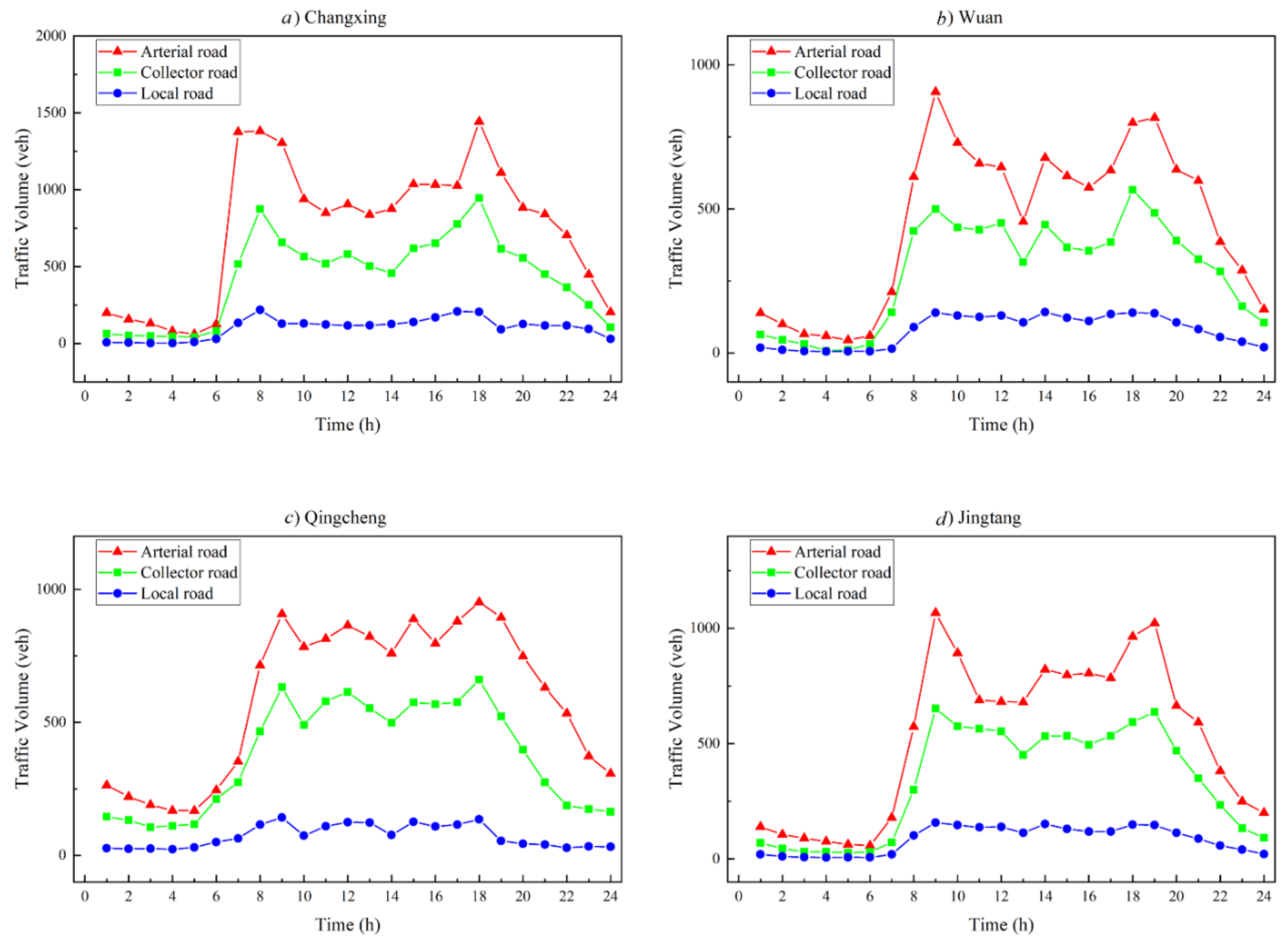
Figure 2 depicts road traffic volume conditions in different time periods in Changxing, Wuan, Qingcheng, and Jintang county. The traffic data were obtained from the bayonet system of the Vehicle Management Office in each county. It can be easily found that there are obvious morning and evening peaks in these four counties. Therefore, according to the travel characteristics presented in Figure 2, the periods 7:00–9:00 a.m. and 17:00–19:00 p.m. are set as peak hour periods, 22:00 p.m.–6:00 a.m. is selected as a free flow period, and other times are set as off-peak hours.
In China, the LOS is divided into four levels ranging from 1 to 4, and the corresponding recommended value of V/C is presented in Table 4. Note that the value of V/C is usually obtained through field observations.
To derive the actual traffic volume, it is necessary to know the service level or V/C ratio of different road types at different times. In general, the intention of road traffic planning is to alleviate road traffic congestion and thus improve LOS. All of the planning indicators are usually designed to meet peak-hour demand so that the LOS at the peak hours cannot exceed the third level, whose average V/C is 0.8. Therefore, 0.8 is adopted in this paper for the V/C on arterial roads during peak hours in the planning year. It is assumed that the travel characteristics will not change much in counties if there are no traffic control measures (e.g., vehicle limit). Therefore, the current travel characteristics can be applied to derive the V/C value on other road types and during different times based on the given V/C for arterial roads during peak hours, as shown in Equation (5).
where and represents the V/C value and the average traffic volume on road classification during period , respectively. represents the arterial road, collector road, and local road, respectively. stands for the different hourly periods, i.e., peak, off-peak, and free flow period, respectively. For example, is the V/C value of arterial road during peak hours. stands for the possible capacity of road classification .
Then, we averaged the parameters derived from the traffic volume data of the four counties, and the final results of the V/C value of different road types during different times adopted in this paper are presented in Table 5.
Note that the unit of the capacity is instead of —in order to facilitate the calculation of GHG emissions of different vehicle categories, it is necessary to derive the actual traffic volume for different vehicle categories based on the vehicle conversion factors. In this paper, we adopted the recommended values in “Urban Road Engineering Design Specifications (CJJ37-2012)” [34]. The conversion factors for LDPV, LDT, and MC are 1.0, 1.2, and 0.4, respectively.
Based on the above analysis, the hourly traffic volume on each classification of urban roads could thus be derived, as shown in Equation (6).
where and stand for one-way traffic volume and V/C value on road classification during period , respectively. represents the possible one-way section throughput of road classification , and and refer to the proportion and vehicle conversion factor of vehicle category , respectively.
Then, hourly vehicle kilometers travel (VKT) can be derived:
where is the vehicle distance traveled by vehicle category during period , and represents the length of road classification .
2.3.2. Prediction of Average Speed Distribution on Different Road Types
As mentioned in Section 2.2, vehicle emissions are closely related to its driving speed. Generally, the lower the speed, the higher the emissions, especially at the idling process, the emissions will increase exponentially. In addition, vehicles driving on different types of roads (with different speed limits or expectations) during different time periods (with different traffic conditions) will produce different speed distributions. In this study, the method of simulation by VISSIM was adopted to obtain the average speed distribution on different road types.
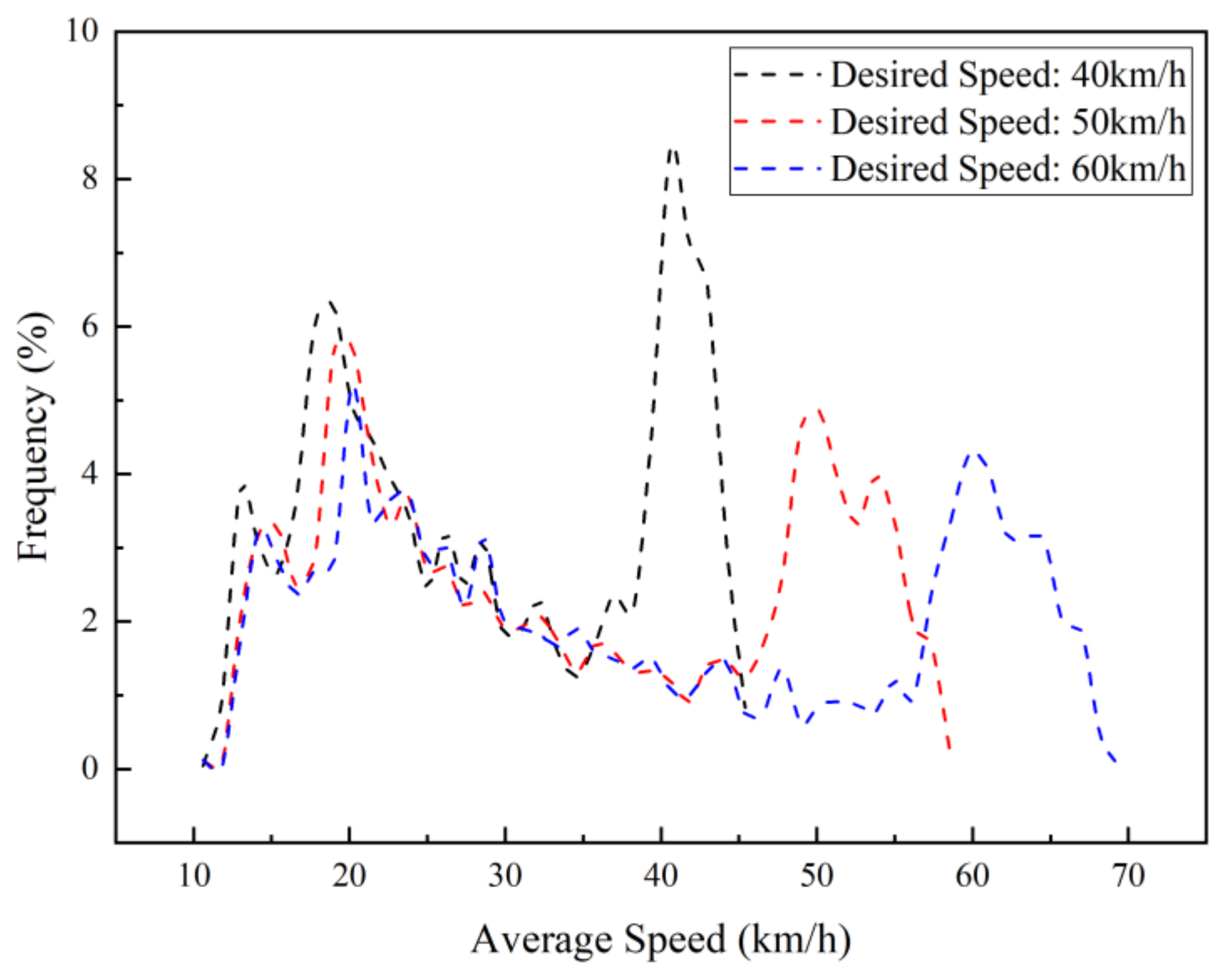
Figure 3 shows three typical average speed distribution at a different desired speeds. The blue, red, and black dotted lines indicate the average speed distributions at the desired speeds of 60 km/h, 50 km/h, and 40 km/h, respectively. Through the analysis of the simulation results, we can find that the vehicle with the average speed in the range of 10–30 km/h will reach the intersection when the signal light is red. On the contrary, the vehicle with the average speed in the interval of 30–60 km/h will pass the intersection during the green light signal. From Figure 3, it can be clearly seen that the distribution of velocity in the interval of 10–30 km/h is roughly consistent at different expected speeds. For different roads at a different desired speed, the biggest difference in the average speed distribution is the distribution that the vehicle passes through the intersection without idling. Therefore, we must conduct a simulation analysis for different road types under different traffic conditions.
In VISSIM, changing the random seed to the same road segment file may derive different results of each simulation. This is because the arrival rules of vehicles are different if we use a different random seed. Through statistical analysis of average values, it can be more reasonable to reflect the average operating condition of the actual or designed traffic system in a certain period. To eliminate the influence of other random factors on the simulation test results, we used the method of changing the random seed to carry out a simulation test to verify the validity of our simulation results. Figure 4 depicts the average speed distribution under the simulation of 1 random seed and 99 random seeds, respectively. It can be easily found that changes in random seeds have less effect on the results of vehicle average speed distribution.
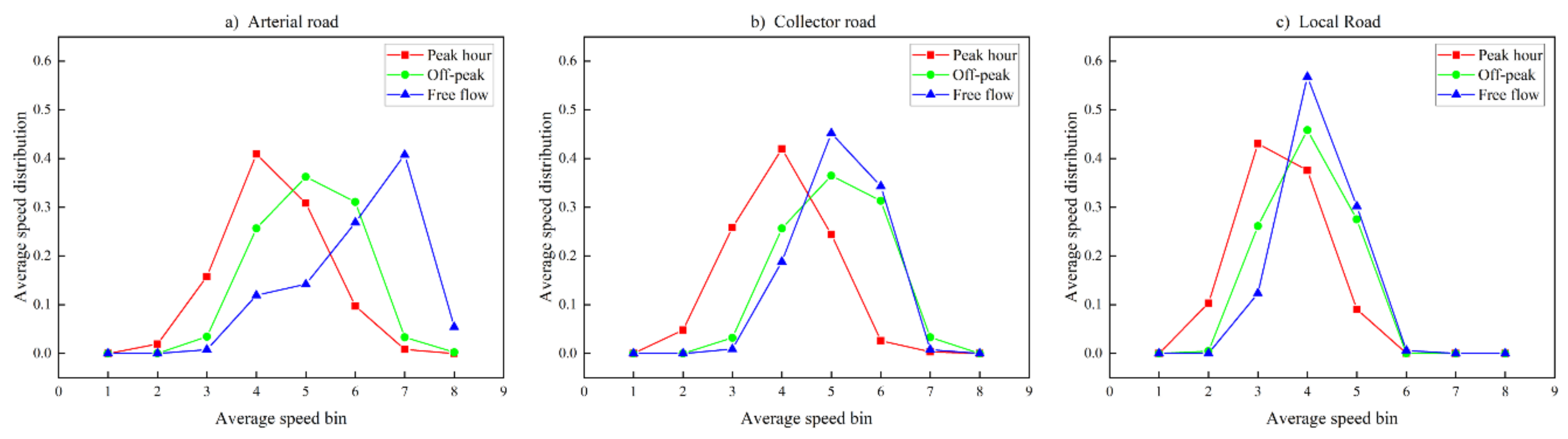
We carried out multiple simulations on the arterial road, collector road, and local road according to the estimated traffic volume during peak hours, off-peak periods, and free flow periods, and finally obtained the average speed distribution of different road sections during different time periods, as shown in Figure 5.
3. Case Study
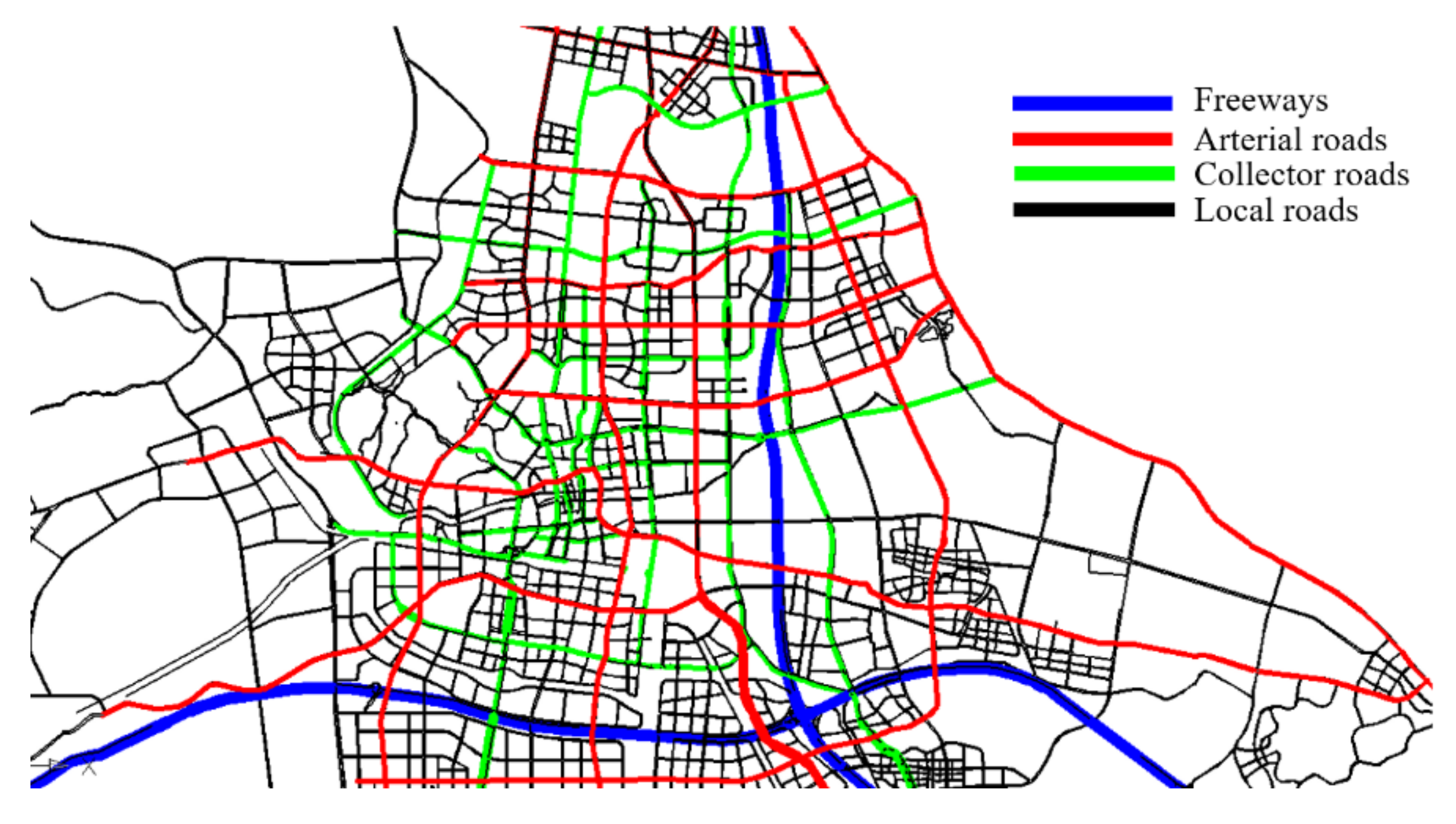
Changxing county, one of the largest and most developed counties in Yangtze River Delta, was selected as the representative county for the case study to validate our proposed method. Figure 6 presents its urban road network plan in 2020. The total length of arterial roads, collector roads, and local roads are 230.5 km, 138.78 km, and 312 km, respectively. The lane number of arterial roads, collector roads, and local roads are 6, 4, and 2, respectively. The design speed of arterial roads, collector roads, and local roads are 60 km/h, 40 km/h, and 30 km/h, respectively.
Based on Table 3, Table 5, Equation (6), and Equation (7), the VKT on different road types during the different time periods can be derived, as shown in Table 6.
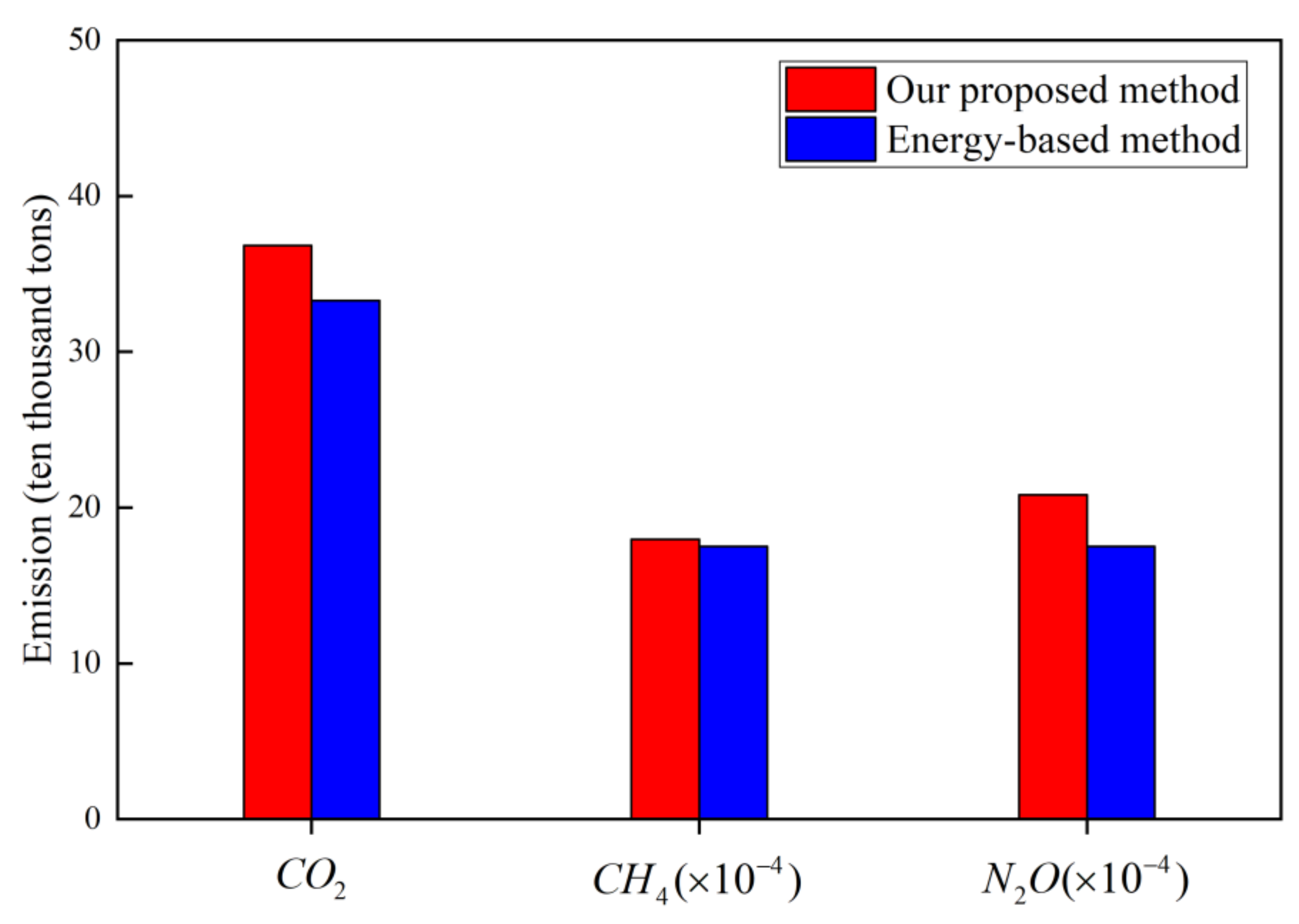
Then, the average speed distribution (see Figure 5) and its corresponding emission rates (see Table 2) can be applied to derive the GHG emissions using the calculation method as shown in Equation (2). The final results of CO2, CH4, and N2O emissions are 368.2600 kt, 0.0179 kt, and 0.0208 kt.
To demonstrate the effectiveness of the method developed in Section 2, the energy-based method [35] was adopted as a benchmark to compare with our results. The total fuel consumption was multiplied by the fuel carbon emission factor to calculate the carbon emissions, as mentioned in Section 1. Hence, if we want to predict emissions in the coming years, it necessary to predict the fuel consumption data by all vehicles, that is, we need to predict future motor vehicle ownership. A motor vehicle ownership prediction method based on support vector machines (SVMs) proposed by Zhang et al. [36] was adopted, and the total number of LDPV, LDT, and MC ownership will reach 192,910 by 2020.
According to Changxing’s motor vehicle registration data, the total number of LDPV, LDT, and MC powered by gasoline in 2017 was 177,289 and its corresponding gasoline consumption was 93,828 tons according to the statistics of energy consumption in Changxing. According to the motor vehicle data and energy consumption statistics of Changxing County in recent years, energy consumption is almost proportional to the number of motor vehicles. Thus, it is assumed that the fuel consumption is also proportional to the number of vehicles in this paper. It can be inferred that the gasoline consumption data in the planning year is 102,095 tons. Then, the total energy released during gasoline combustion could be derived from its heating value (44,000 kJ/kg is adopted), the result is 4492.190 TJ. Finally, the emissions can thus be derived from the emission factors recommended in IPCC (74,100 kg/TJ for CO2, 3.9 kg/TJ for CH4, and 3.9 kg/TJ for N2O), the final results are shown in Figure 7. Note that to better show the results, we multiplied the values of CH4 and N2O by 10,000.
From Figure 7, it can be found that the two methods have almost the same results, except that the carbon dioxide prediction error is slightly larger. We believe that such an error is reasonable and is within an acceptable range. Therefore, it can be concluded that our method is feasible. However, it is worth noting that although the final total emission results we get are almost the same, the energy-based method cannot capture the detailed or fine-grained information of the emissions, such as the emissions on different road types or the emissions during different time periods. This information is often needed by transportation planning designers, and they can help them make better decisions during the low-carbon transportation planning process.
4. Applications
4.1. Application to GHG Driving Factors Analysis
There are many factors affecting the carbon emissions of road networks, such as the level of economic development, motor vehicle ownership, road mileage, as well as arterial road ratio. In this section, we apply the same method proposed in Section 2 to thirty other counties in China in order to calculate the GHG emissions in these counties. Then, we conduct the driving factor analysis to derive the most important factors, which are of great significance for establishing an effective GHG emission prediction model and developing low-carbon traffic road planning in the future.
County Selection
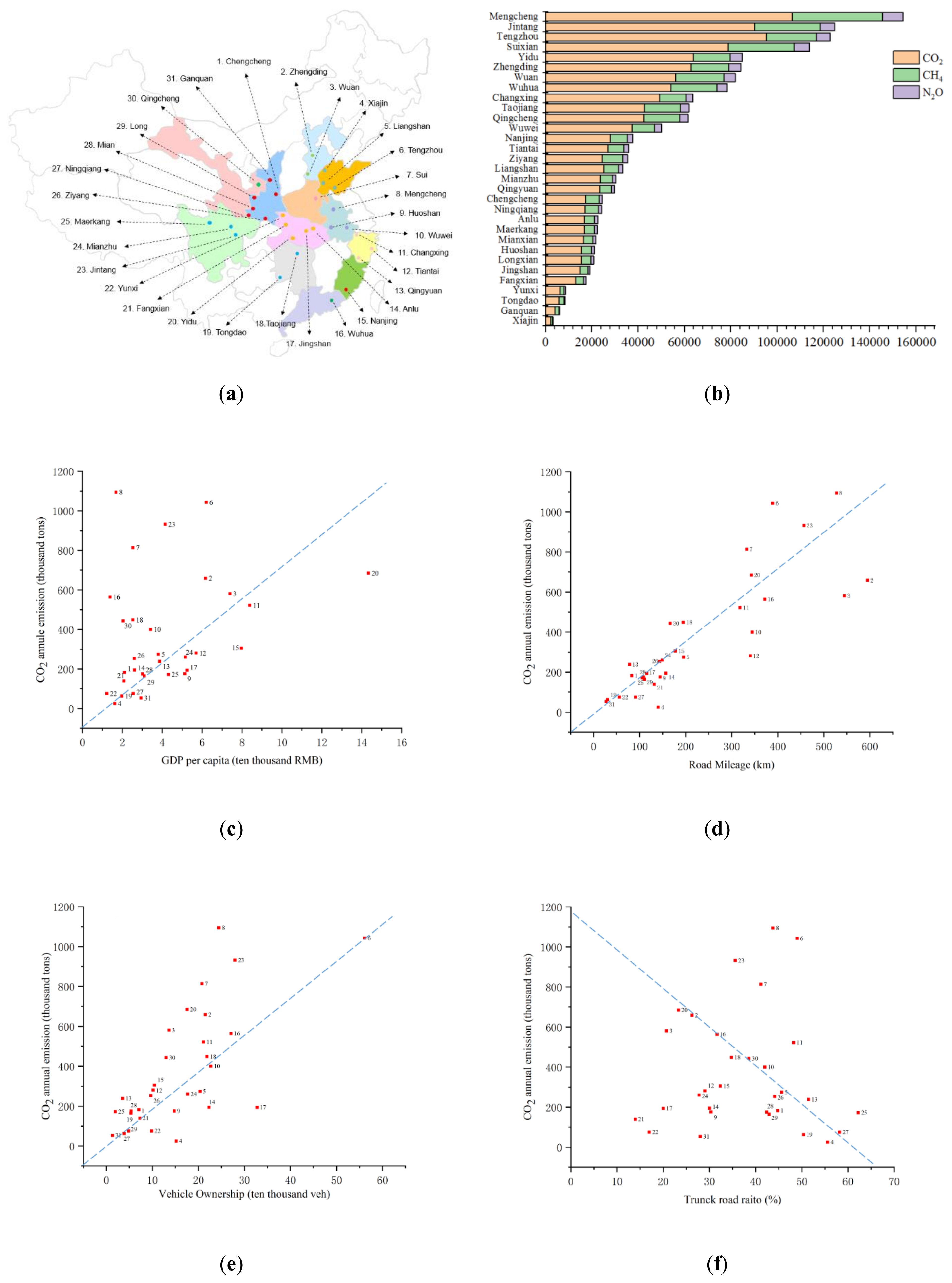
In order to better analyze the driving factors, when selecting the county, we first ensured that the road traffic indicators mentioned in Section 2 were all available in the comprehensive traffic planning of every county. On the basis of ensuring this precondition, taking into account different levels of economic development and different geographical characteristics become our choice to explore the impact of economic development level and regional characteristics. In the end, in addition to Changxing, we chose 30 counties as follows: Shanxi province (Long county, Chenghceng county, Ganquan county, Mian county, Ningqiang county, Ziyang county); Sichuan province (Jintang county, Maerkang county, Mianzhu county); Hubei province (Jingshan county, Anlu county, Yunxi county, Fang county, Yidu county); Anhui province (Wuwei county, Huoshan county, Mengcheng county); Shandong province (Tengzhou county, Liangshan county, Xiajin county); Guangdong province (Wuhua county); Hunan province (Tongdao county, Taojiang county); Hebei province (Zhengding county, Wuan county); Fujian province (Nanjing county); Zhejiang province (Tiantai county, Changxing county, Qingyuan county); Henan province (Suixian county); and Gansu province (Qingcheng county). For convenience, we used the numbers 1 to 31 to represent the counties above in alphabetical order, as shown in Figure 8a. The transportation planning indicators were obtained from the comprehensive transportation planning text of each county (see Table S2 in the Supplementary Data file).
Figure 8b shows the annual GHG emissions in 31 counties. Figure 8c–f depicts the relationship between GDP per capita, road mileage, vehicle ownership, arterial road ratio, and annual CO2 emissions of 31 counties, respectively. It could be found that the emissions were significantly positively correlated with GDP per capita, road mileage, and vehicle ownership in 31 counties. Some counties deviated from the line. This is because carbon emissions are affected by many factors. For example, some counties like Tengzhou and Mengcheng, their road mileage is relatively higher. As road mileage is the main indicator in the traffic planning process, unrestricted road construction will increase carbon emissions according to the growth trend line in Figure 8d. As the urbanization level increases in China, Chinese counties are gradually showing an expansion trend, and emissions from road transportation shall undoubtedly continue to boost unless some effective control measures are implemented. On the other hand, from the Figure 8f, it could be found that arterial road is able to bring benefits to curb road transportation carbon emissions in counties to a certain extent. Therefore, it is of great importance for Chinese counties to better balance the proportion of different grades of urban roads in the road traffic planning process. In order to ensure that the travel needs of residents are met, we should consider increasing the service level of all grade roads as much as possible to reduce congestion, increase the average operating speed, and thus reduce the total carbon emissions.
4.2. Application to Peak Hour Emission Coefficient
As described in Section 2, calculating carbon emissions from road traffic throughout a year is not a simple process but a computationally intensive process. It requires a cumulative amount of hourly emission data, which is a time-consuming and labor-intensive process. Thus, how to find a more concise way to estimate annual carbon emissions is an important and meaningful issue to be investigated.
Traffic volume has the characteristics of changing with time and peak hours. This must be considered when designing road facilities. As the driving factor analysis above shows, road traffic carbon emissions are closely related to traffic volume. Motivated by the conception of design-hour volume (DHV) in road traffic planning, in this paper we propose the concept of peak hour GHG emission coefficient, which can be calculated as:
where is the average peak hour GHG emission (g/h), denotes average daily GHG emissions of the planning year (g/day), and represents the peak hour GHG emission coefficient.
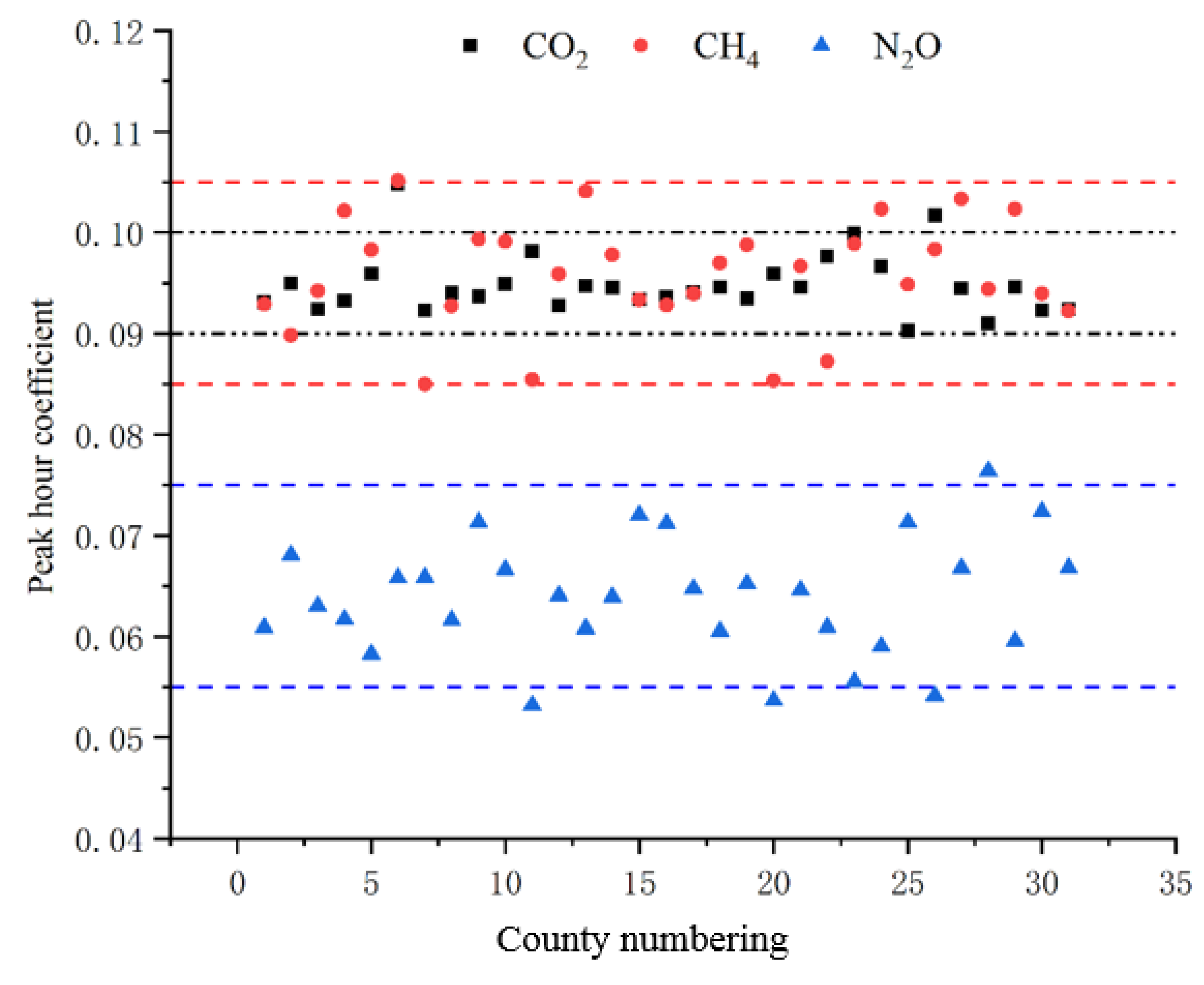
Based on the GHG emission prediction methodology we developed in Section 2, we recalculated peak hour carbon emissions of each county during its morning peak hours. Figure 9 depicts the peak hour emission coefficient of CO2, CH4, and N2O. It can be found that the peak hour coefficients of CO2, CH4, and N2O in these 31 counties are all stable within a certain range. Among them, the peak hour emission coefficient of CO2, CH4, and N2O is distributed in 0.09–0.10, 0.08–0.11, and 0.05–0.08, respectively.
In road traffic planning, all of our planning indicators are generally indicators that meet the maximum demand for travel during peak hours. However, our carbon control indicator is a year-round indicator or a daily average carbon emission indicator. Thus, our analysis results in this section could play the role of a bridge that connects the peak hour’s carbon emissions and annual carbon emissions. Using the peak hour emission coefficient, it is possible to collect only the traffic activity data during peak hours, rather than 24 h a day. It eliminates the most significant barrier for data collection burden and provides a pathway for convenient assessment for annual GHG emissions.
5. Conclusions
Based on urban road transportation planning indicators and open-access emission rates of MOVES, this study developed a novel prediction methodology of hourly GHG emissions from on-road vehicles over the urban roads network of counties and discussed its two possible applications. The case study in Changxing county shows the effectiveness of our proposed method, and the results of driving factors analysis of emissions indicate that the urban road mileage and arterial road ratio are the two most important factors affecting road network GHG emissions in road traffic planning process, requiring special attention for transportation planning designers. The results of hourly emissions analysis indicate that the heavy travel demand during peak hours leads to intensive emissions. The peak hour emission of CO2, CH4, and N2O accounts for approximately 9–10%, 8.5–10.5%, 5.5–7.5% of daily emissions, respectively. Therefore, the control of travel demand during peak hours can effectively reduce emissions, which is the problem to be solved by low-carbon transportation planning. The peak hour emission coefficient can be adopted for quickly estimating daily or annual emissions, greatly reducing the calculation workload.
It is worth noting that our proposed method is not only applicable to the estimation of the road traffic carbon emissions in the planning year but also to existing road networks if current road network indicator data are available. It is expected to promote the implementation of effective low-carbon measures and the development of a sustainable transportation system.
There are some limitations to this study that would need further improvements. First, more available traffic data need to be collected for the purpose of more accurate prediction. This issue will be easier to achieve in the future connected and automated environment. In addition, this study is performed under traditional traffic environment. Therefore, further study may focus on the analysis of the impact of connected and automated vehicles on GHG emissions and try to propose a prediction method of emissions under a connected and automated environment to further expand the research of this study. There are also some other interesting topics that call for more attention in the connected and automated environment in the near future. The transportation planning method as well as the innovation and development of traffic control in a connected environment are two interesting research topics for the sustainable transportation development. Nevertheless, this paper provides a general framework for the traffic GHG emission prediction method.
Supplementary Materials
The following are available online at https://0-www-mdpi-com.brum.beds.ac.uk/2071-1050/12/24/10251/s1, Table S1: The average speed bin description in MOVES, Table S2: The trasporation planning indicators in 31 counties.
Author Contributions
Conceptualization, J.G. and L.L.; methodology, J.G.; software, L.L.; validation, J.G. and Q.X.; formal analysis, J.G.; investigation, L.L.; data curation, J.G.; writing—Original draft preparation, J.G.; writing—Review and editing, B.R.; visualization, L.L.; supervision, Q.X.; project administration, Q.X.; funding acquisition, Q.X. All authors have read and agreed to the published version of the manuscript.
Funding
This study was carried out with the support of the National Key R&D Program of China (Grant No. 2018YFC0704704). In addition, the authors would like to express their appreciation to the MOVES Team for providing the MOVES2014 documentation and for their technical assistance regarding emission regulations and measurements.
Acknowledgments
Part of the research was conducted at the University of Wisconsin-Madison where the first author spent a year as a visiting scholar funded by the China Scholarship Council.
Conflicts of Interest
The authors declare no conflict of interest.
References
- Rubio, E.V.; Rubio, J.M.Q.; Moreno, V.M. Environmental fiscal effort: Spatial convergence within economic policy on taxation. Rev. Econ. Mund. 2017, 45, 87–100. [Google Scholar]
- Helfaya, A.; Whittington, M. Does designing environmental sustainability disclosure quality measures make a difference? Bus. Strategy Environ. 2019, 28, 525–541. [Google Scholar] [CrossRef]
- Janik, A.; Ryszko, A.; Szafraniec, M. Greenhouse gases and circular economy issues in sustainability reports from the energy sector in the European Union. Energies 2020, 13, 5993. [Google Scholar] [CrossRef]
- Birol, F. CO2 Emissions from Fuel Combustion; IEA: Paris, France, 2019; pp. 1–165. [Google Scholar]
- Martín, J.M.M.; Guaita-Martinez, J.M.; Molina-Moreno, V.; Rodríguez, A.S. An analysis of the tourist mobility in the Island of Lanzarote: Car rental versus more sustainable transportation Alternatives. Sustainability 2019, 11, 739. [Google Scholar] [CrossRef] [Green Version]
- Ruiz-Guerra, I.; Molina-Moreno, V.; Cortés-García, F.J.; Núñez-Cacho, P. Prediction of the impact on air quality of the cities receiving cruise tourism: The case of the Port of Barcelona. Heliyon 2019, 5, e01280. [Google Scholar] [CrossRef] [Green Version]
- Nakamura, K.; Hayashi, Y. Strategies and instruments for low-carbon urban transport: An international review on trends and effects. Transp. Policy 2013, 29, 264–274. [Google Scholar] [CrossRef]
- Brand, C.; Anable, J.; Tran, M. Accelerating the transformation to a low carbon passenger transport system: The role of car purchase taxes, feebates, road taxes and scrappage incentives in the UK. Transp. Res. Part A Policy Pract. 2013, 49, 132–148. [Google Scholar] [CrossRef]
- Wang, P. Research on Urban Road Network Structure Optimization Based on the Concept of Low-Carbon; Chongqing Jiaotong University: Chongqing, China, 2015. [Google Scholar]
- Zhang, X.; Liu, P.; Li, Z.; Yu, H. Modeling the effects of low-carbon emission constraints on mode and route choices in transportation networks. Procedia Soc. Behav. Sci. 2013, 96, 329–338. [Google Scholar] [CrossRef] [Green Version]
- Zhang, S.; Wu, Y.; Hu, J.; Huang, R.; Zhou, Y.; Bao, X.; Fu, L.; Hao, J. Can Euro V heavy-duty diesel engines, diesel hybrid and alternative fuel technologies mitigate NOX emissions? New evidence from on-road tests of buses in China. Appl. Energy 2014, 132, 118–126. [Google Scholar] [CrossRef]
- Costa, M.; Sorge, U.; Allocca, L. Increasing energy efficiency of a gasoline direct injection engine through optimal synchronization of single or double injection strategies. Energy Convers. Manag. 2012, 60, 77–86. [Google Scholar] [CrossRef]
- Zhou, Y.; Wu, Y.; Yang, L.; Fu, L.; He, K.; Wang, S.; Hao, J.; Chen, J.; Li, C. The impact of transportation control measures on emission reductions during the 2008 Olympic Games in Beijing, China. Atmos. Environ. 2010, 44, 285–293. [Google Scholar] [CrossRef]
- Tonne, C.; Beevers, S.; Armstrong, B.; Kelly, F.J.; Wilkinson, P. Air pollution and mortality benefits of the London Congestion Charge: Spatial and socioeconomic inequalities. Occup. Environ. Med. 2008, 65, 620–627. [Google Scholar] [CrossRef] [PubMed]
- Henriksson, G.; Hagman, O.; Andréasson, H. Environmentally reformed travel habits during the 2006 congestion charge trial in Stockholm—A qualitative study. Int. J. Environ. Res. Public Health 2011, 8, 3202–3215. [Google Scholar] [CrossRef] [PubMed]
- Tran, N.H.; Yang, S.-H.; Huang, T. Comparative analysis of traffic-and-transportation-planning-related indicators in sustainable transportation infrastructure rating systems. Int. J. Sustain. Transp. 2020, 7, 1–14. [Google Scholar] [CrossRef]
- Köhler, J.; Turnheim, B.; Hodson, M. Low carbon transitions pathways in mobility: Applying the MLP in a combined case study and simulation bridging analysis of passenger transport in the Netherlands. Technol. Forecast. Soc. Chang. 2020, 151, 119314. [Google Scholar] [CrossRef] [Green Version]
- IPCC. 2006 IPCC Guidelines for National Greenhouse Gas Inventories. 2006. Available online: https://www.ipcc-nggip.iges.or.jp/public/2006gl/chinese/index.html (accessed on 8 December 2020).
- Zeng, Y.; Tan, X.; Gu, B.; Wang, Y.; Xu, B. Greenhouse gas emissions of motor vehicles in Chinese cities and the implication for China’s mitigation targets. Appl. Energy 2016, 184, 1016–1025. [Google Scholar] [CrossRef]
- Peng, T.; Ou, X.; Yuan, Z.; Yan, X.; Zhang, X. Development and application of China provincial road transport energy demand and GHG emissions analysis model. Appl. Energy 2018, 222, 313–328. [Google Scholar] [CrossRef]
- Zhang, H.; Kong, X.; Ren, C. Influencing factors and forecast of carbon emissions from transportation-Taking Shandong province as an example. IOP Conf. Ser. Earth Environ. Sci. 2019, 300, 1–6. [Google Scholar] [CrossRef]
- Zheng, B.; Huo, H.; Zhang, Q.; Yao, Z.L.; Wang, X.T.; Yang, X.; Liu, H.; He, K.B. High-resolution mapping of vehicle emissions in China in 2008. Atmos. Chem. Phys. Discuss. 2014, 14, 9787–9805. [Google Scholar] [CrossRef] [Green Version]
- Gong, M.; Yin, S.; Gu, X.; Xu, Y.; Jiang, N.; Zhang, R. Refined 2013-based vehicle emission inventory and its spatial and temporal characteristics in Zhengzhou, China. Sci. Total Environ. 2017, 599–600, 1149–1159. [Google Scholar] [CrossRef]
- Yang, W.; Yu, C.; Yuan, W.; Wu, X.; Zhang, W.; Wang, X. High-resolution vehicle emission inventory and emission control policy scenario analysis, a case in the Beijing-Tianjin-Hebei (BTH) region, China. J. Clean. Prod. 2018, 203, 530–539. [Google Scholar] [CrossRef]
- Liu, Y.; Ma, J.-L.; Li, L.; Lin, X.-F.; Xu, W.-J.; Ding, H. A high temporal-spatial vehicle emission inventory based on detailed hourly traffic data in a medium-sized city of China. Environ. Pollut. 2018, 236, 324–333. [Google Scholar] [CrossRef]
- Kholod, N.; Evans, M.H.; Gusev, E.P.; Yu, S.; Malyshev, V.L.; Tretyakova, S.; Barinov, A. A methodology for calculating transport emissions in cities with limited traffic data: Case study of diesel particulates and black carbon emissions in Murmansk. Sci. Total Environ. 2016, 547, 305–313. [Google Scholar] [CrossRef] [Green Version]
- Gong, M.; Liu, H.; Atif, R.M.; Jiang, X. A study on the factor market distortion and the carbon emission scale effect of two-way FDI. Chin. J. Popul. Resour. Environ. 2019, 17, 145–153. [Google Scholar] [CrossRef]
- Gill, A.R.; Viswanathan, K.K.; Hassan, S. A test of environmental Kuznets curve (EKC) for carbon emission and potential of renewable energy to reduce green house gases (GHG) in Malaysia. Environ. Dev. Sustain. 2017, 20, 1103–1114. [Google Scholar] [CrossRef]
- Huo, H.; Zhang, Q.; He, K.; Yao, Z.; Wang, X.; Zheng, B.; Streets, D.G.; Wang, Q.; Ding, Y. Modeling vehicle emissions in different types of Chinese cities: Importance of vehicle fleet and local features. Environ. Pollut. 2011, 159, 2954–2960. [Google Scholar] [CrossRef] [PubMed]
- Wang, S.; Huang, Y.; Zhou, Y. Spatial spillover effect and driving forces of carbon emission intensity at the city level in China. J. Geogr. Sci. 2019, 29, 231–252. [Google Scholar] [CrossRef] [Green Version]
- EPA. MOVES and Other Mobile Source Emissions Models. Available online: https://www.epa.gov/moves (accessed on 8 December 2020).
- Pinto, G.; Oliver-Hoyo, M.T. Using the relationship between vehicle fuel consumption and CO2 emissions to illustrate chemical principles. J. Chem. Educ. 2008, 85, 218–220. [Google Scholar] [CrossRef]
- Beijing Municipal Design and Research Institute. Urban Road Design Specifications (CJJ 36-90); China Construction Industry Press: Beijing, China, 2006. [Google Scholar]
- Ministry of Housing and Urban-Rural Development of the People’s Republic of China. Urban Road Engineering Design Specifications (CJJ37-2012); China Construction Industry Press: Beijing, China, 2016.
- IPCC. 2019 Refinement to the 2006 IPCC Guidelines for National Greenhouse Gas Inventories. Available online: http://www.ipcc.ch/report/2019-refinement-to-the-2006-ipcc-guidelines-for-national-greenhouse-gas-inventories/ (accessed on 8 December 2020).
- Zhang, X.H.; Hu, M.Q.; Peng, X.Y.; Gan, J.; Xiang, Q.J. Prediction of motor vehicle ownership in county towns based on support vector machine. In Proceedings of the 4th International Conference on Intelligent Transportation Engineering (ICITE), Singapore, 6–8 September 2018; pp. 311–315. [Google Scholar]
Figure 1.
Flow diagram of the methodology.

Figure 2.
Road traffic volume condition in different time periods in different counties.

Figure 3.
Average speed distribution under the different desired speed.

Figure 4.
Average speed distribution under different random seed of simulations.

Figure 5.
Average speed distribution on different road type during different time periods.

Figure 6.
The urban road network plan of Changxing County in 2020.

Figure 7.
The comparative results of our proposed method to the energy-based method.

Figure 8.
The GHG Emissions in 31 counties and driving factors analysis. (a) Location of the 31 counties we selected; (b) annual GHG emissions in 31 counties; (c) CO2 emission-GDP per capita; (d) CO2 emission-road mileage; (e) CO2 emission-vehicle ownership; (f) CO2 emission-arterial road ratio.
Figure 8.
The GHG Emissions in 31 counties and driving factors analysis. (a) Location of the 31 counties we selected; (b) annual GHG emissions in 31 counties; (c) CO2 emission-GDP per capita; (d) CO2 emission-road mileage; (e) CO2 emission-vehicle ownership; (f) CO2 emission-arterial road ratio.

Figure 9.
Peak hour emission coefficient of CO2, CH4, and N2O.


Table 1.
Definition of vehicle categories in this study.
| Vehicle Category | Abbreviation | Description | Fuel Type |
|---|---|---|---|
| Light-duty passenger vehicle | LDPV | Any coupe, compact car, sedan, SUVs, minivans whose primary purpose is to carry passengers | gasoline |
| Light-duty truck | LDT | Trucks with a gross vehicle weight rating (GVWR) less than 8500 pounds | gasoline |
| Motorcycle | MC | All two- or three-wheeled motorized vehicles | gasoline |
Table 2.
Benchmark fuel consumption and speed correction functions for LDPV, LDT, and MC.
| Vehicle Category | Fuel Type | Benchmark Speed Bin | Benchmark Fuel Consumption (L/100 km) | Speed Correction Functions |
|---|---|---|---|---|
| LDPV | Gasoline | 5 | 8.86 | 4.38495x−0.90741 |
| LDT | Gasoline | 5 | 10.87 | 4.27765x−0.89292 |
| MC | Gasoline | 5 | 3.82 | 3.98090x−0.74419 |
Note: 16 average speed bin are defined in MOVES for emission rates, ranging from 4− to 120 + km/h (see Table S1 in the Supplementary Data file).
Table 3.
Basic capacity and its correction factors of counties in China.
| Parameter | Arterial Road | Arterial Road | Collector Road | Local Road |
|---|---|---|---|---|
| Lane number (one-way) | 3 | 2 | 2 | 1 |
| (km/h) | 50 | 50 | 40 | 30 |
| (pcu/h/lane) | 1690 | 1690 | 1640 | 1550 |
| 2.60 | 1.87 | 1.87 | 1.00 | |
| 0.75 | 0.75 | 0.75 | 0.75 | |
| 0.90 | 0.90 | 0.80 | 0.70 | |
| 0.52 | 0.52 | 0.68 | 0.65 | |
| 0.90 | 0.90 | 0.85 | 0.80 | |
| 0.95 | 0.95 | 0.95 | 0.9 | |
| (pcu/h) | 1319 | 948 | 1010 | 380 |
Table 4.
Level of service (LOS) classification and its corresponding volume to capacity ratio (V/C).
Table 4.
Level of service (LOS) classification and its corresponding volume to capacity ratio (V/C).
| LOS | One | Two | Three | Four |
|---|---|---|---|---|
| V/C | Less than 0.6 | 0.6–0.75 | 0.75–0.9 | Over 0.9 |
Table 5.
The V/C value of different road types during different times in the planning year.
| Time Period | Arterials | Collector Roads | Local Roads |
|---|---|---|---|
| Peak periods | 0.80 | 0.58 | 0.44 |
| Off-peak periods | 0.59 | 0.41 | 0.30 |
| Free-flow periods | 0.13 | 0.08 | 0.05 |
Table 6.
Estimation of vehicle kilometers travel (VKT) during different times over the entire urban road network.
Table 6.
Estimation of vehicle kilometers travel (VKT) during different times over the entire urban road network.
| Road Classification | Arterial Road | Collector Road | Local Road | |||||||
|---|---|---|---|---|---|---|---|---|---|---|
| Period | Peak | Off-Peak | Free Flow | Peak | Off-Peak | Free Flow | Peak | Off-Peak | Free Flow | |
| VKT (veh·km/h) | LDPV | 190,212 | 140,281 | 31,448 | 63,578 | 44,943 | 8922 | 40,797 | 27,816 | 4717 |
| LDT | 20,260 | 14,942 | 3350 | 6772 | 4787 | 950 | 4345 | 2962 | 502 | |
| MC | 20,816 | 15,352 | 3441 | 6958 | 4918 | 976 | 4465 | 3044 | 516 | |
Publisher’s Note: MDPI stays neutral with regard to jurisdictional claims in published maps and institutional affiliations. |
© 2020 by the authors. Licensee MDPI, Basel, Switzerland. This article is an open access article distributed under the terms and conditions of the Creative Commons Attribution (CC BY) license (http://creativecommons.org/licenses/by/4.0/).
Share and Cite
MDPI and ACS Style
Gan, J.; Li, L.; Xiang, Q.; Ran, B. A Prediction Method of GHG Emissions for Urban Road Transportation Planning and Its Applications. Sustainability 2020, 12, 10251. https://0-doi-org.brum.beds.ac.uk/10.3390/su122410251
AMA Style
Gan J, Li L, Xiang Q, Ran B. A Prediction Method of GHG Emissions for Urban Road Transportation Planning and Its Applications. Sustainability. 2020; 12(24):10251. https://0-doi-org.brum.beds.ac.uk/10.3390/su122410251
Chicago/Turabian StyleGan, Jing, Linheng Li, Qiaojun Xiang, and Bin Ran. 2020. "A Prediction Method of GHG Emissions for Urban Road Transportation Planning and Its Applications" Sustainability 12, no. 24: 10251. https://0-doi-org.brum.beds.ac.uk/10.3390/su122410251
Note that from the first issue of 2016, this journal uses article numbers instead of page numbers. See further details here.