A Grid-Based Spatial Analysis for Detecting Supply–Demand Gaps of Public Transports: A Case Study of the Bangkok Metropolitan Region


Abstract
:1. Introduction
- Proposed new public transport performance indicators from the reviewed existing index and analyzed public transport service results.
- Provided an accurate transport planning analysis of the public transport supply–demand and its gaps using the geospatial gridded model (100 m) together with public transport equity measurement.
- The proposed method is well established with possible replication and scale to other cities.
- Demonstrated a real case study of BMR, Thailand with the analysis results for the public transport system.
- The paper’s contents are structured as follows. Section 2 presents a summary of the research context related to public transport measurement and supply–demand gaps analysis. Section 3 provides the details of the methodology used in this study. Section 4 provides the dataset applied in the demonstration. Section 5 then summarizes the results with existing public transport service, supply–demand gaps, and equity. Section 6 discusses the results of the key findings regarding studies on public transport. Section 7 then concludes the research study with recommended indicators for future development and assessment.
2. Related Research
3. Methodology
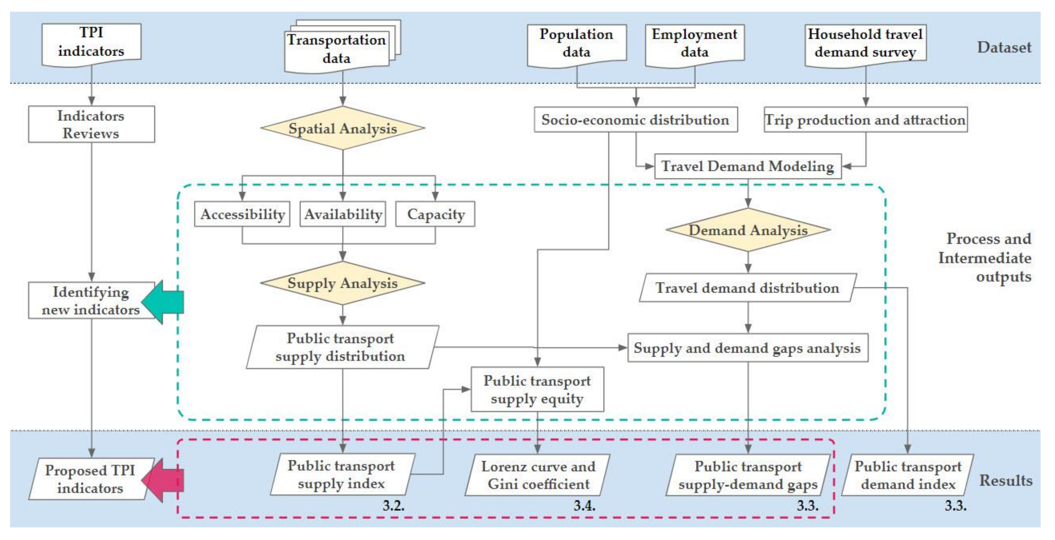
3.1. Overall Methodology
- Method for proposing new TPI indicators
- Method for supply–demand gaps analysis
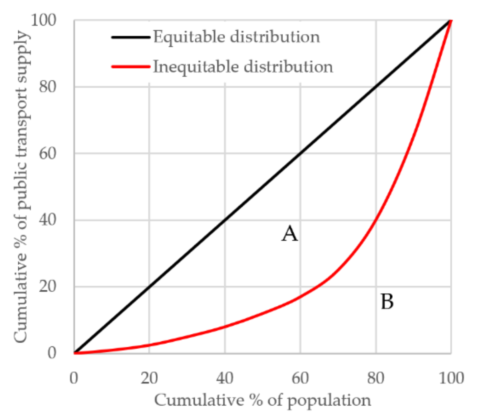
- Lorenz curve and Gini coefficient
3.2. Method for Proposing New TPI Indicators
- 400 m for heavy rail stations, boat piers, and van stations
- 800 m for bus stops and bus rapid transit (BRT) stations
- 1000 m for taxis
- 1500 m for train stations
3.3. Method for Supply–Demand Gaps Analysis
3.4. Lorenz Curves and Gini Coefficient
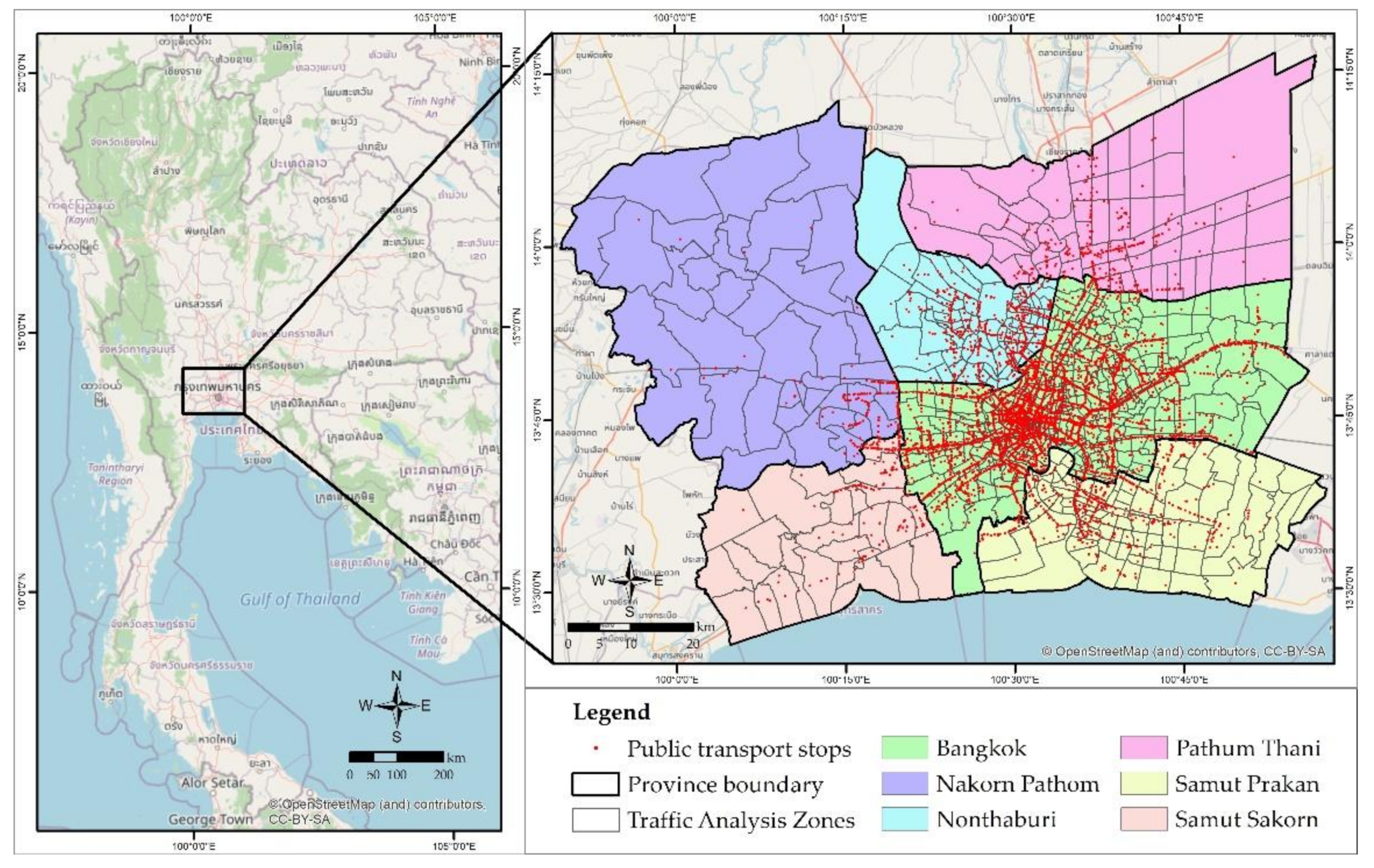
4. Study Area and Dataset
4.1. Study Area
4.2. Dataset for Supply Index
4.2.1. GIS-Based Transportation Data
4.2.2. Transportation Service Information
4.3. Dataset for Demand Index
5. Results
5.1. Proposed New TPI Indicators
5.2. Supply Index
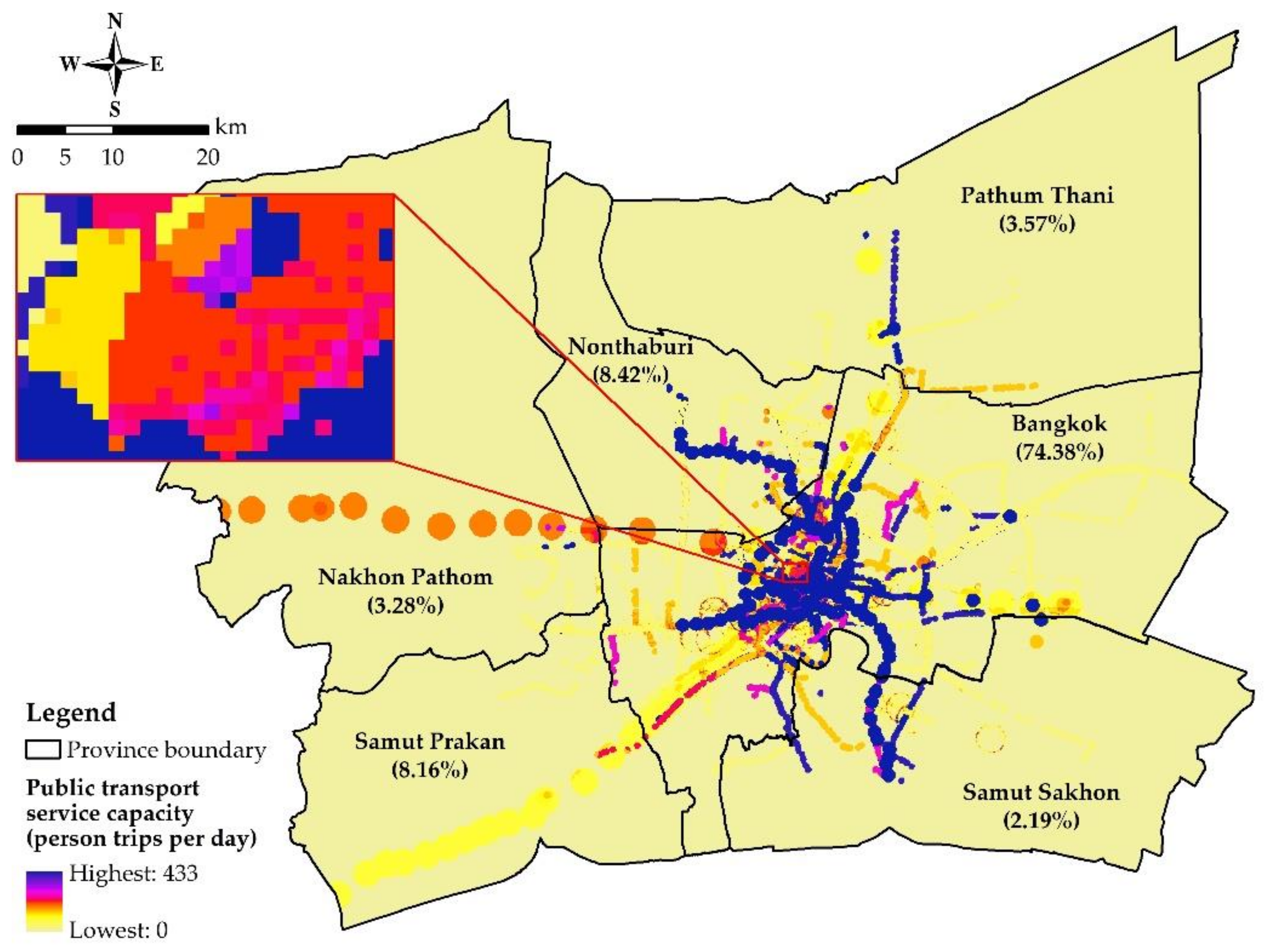
5.2.1. Public Transport Availability and Capacity
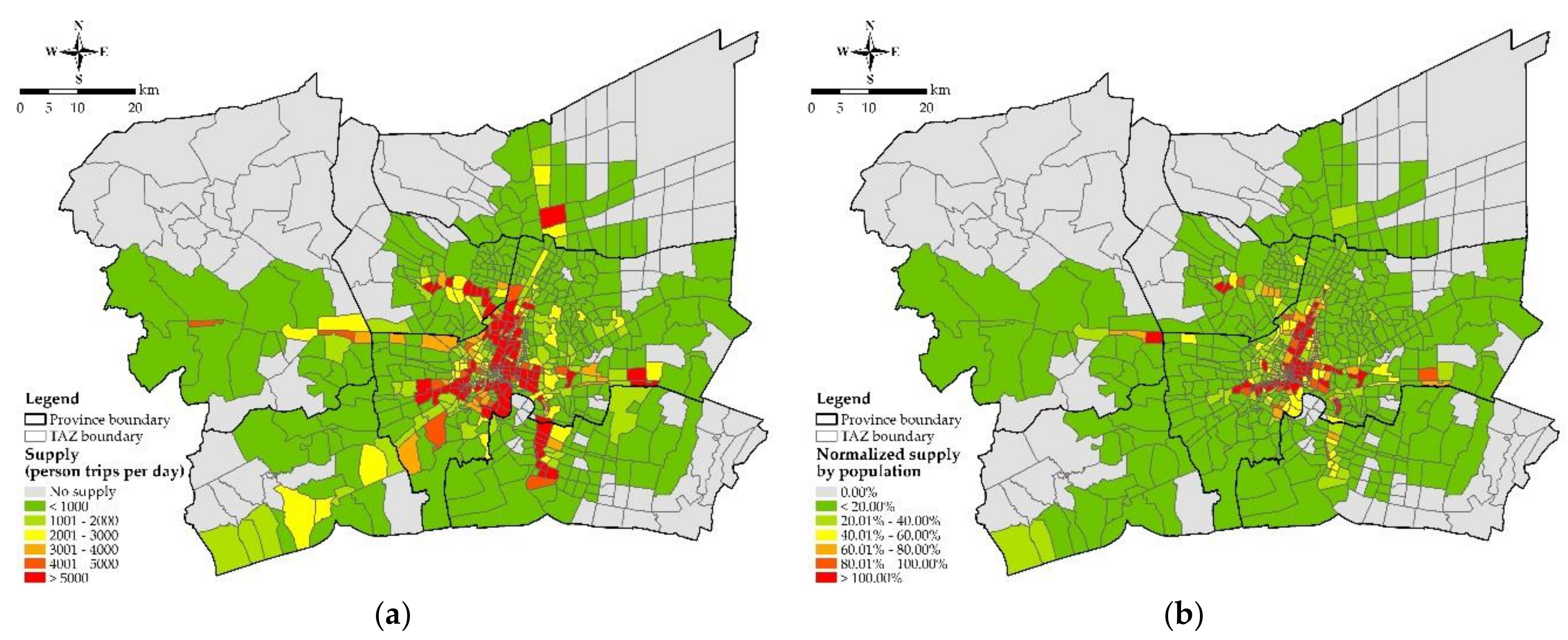
5.2.2. Supply Index and Normalized Supply Index
- In total, 1.6 million residents in Bangkok or about 30% of the population receive zero supply of public transport. Approximately 50% of the population receive a low public transport supply (<20, 20–40), and about 20% of the population receive a high supply of public transport (>40).
- In the Nonthaburi and Samut Prakan provinces, 53% and 65% of the population receive zero supply of public transport, respectively. It was indicated that 40% of residents in Nonthaburi and about 29% of residents in Samut Prakan receive low supply (<20, 20–40). The high public transport supply (>40) serves the population in Nonthaburi and Samut Prakan for 7% and 6%, respectively.
- In the Pathum Thani, Nakhon Pathom, and Samut Sakorn provinces, approximately 84%, 83%, and 73% of the population receive zero supply of public transport, respectively. It was shown that 16% of residents in Nonthaburi and Nakhon Pathom, and 28% of the population in Samut Sakorn receive low supply (<20, 20–40). Interestingly, there has no high public transport supply (>40) that serves residents in Pathum Thani, Nakhon Pathom, and Samut Sakorn provinces.
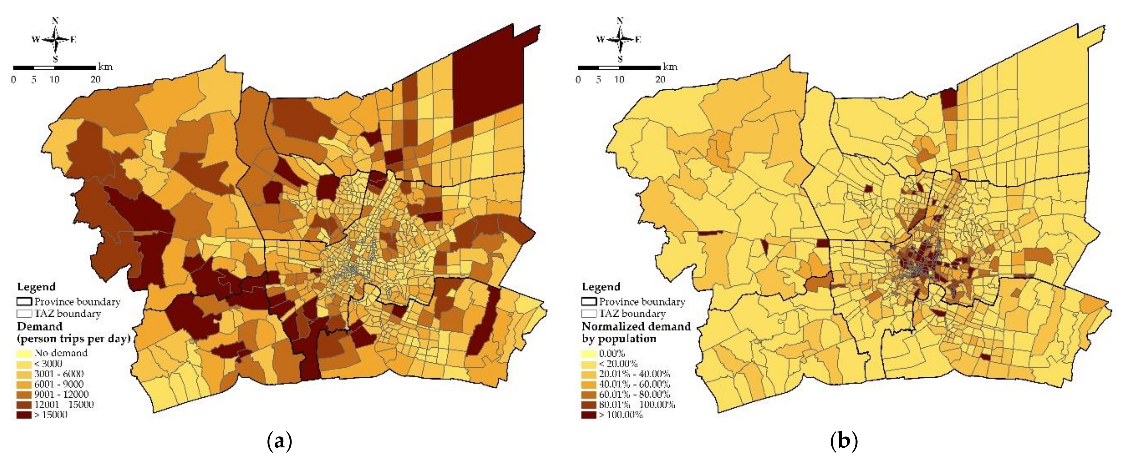
5.3. Demand Index
- In total, 2.5 million residents in Bangkok or about 45% of the residents desire less public transport service (<20). However, 37% of Bangkok residents require moderate public transport service (20–60), while 18% of the population require high public transport service (>60).
- A total of 70% of Nonthaburi residents and 78% of Pathum Thani residents demand less public transport service (<20). Further, 20% of the population in Nonthaburi and 16% of the population in Pathum Thani desire moderate public transport supply (20–60). For the high public transport demand (>60) were sought from 10% and 6% in Nonthaburi and Pathum Thani.
- The populations of Nakhon Pathom, Samut Prakan, and Samut Sakhon require less public transport service (<20), and accounted for 62%, 54%, and 67% share, respectively. In total, 34% of Nakhon Pathom residents, 45% of Samut Prakan residents, and 26% of Samut Sakhon residents seek moderate public transport supply (20–60). A lot less of the population in Nakhon Pathom, Samut Prakan, and Samut Sakhon demand high public transport supply (>60), and account for 4%, 1%, and 7% share of the population, respectively.
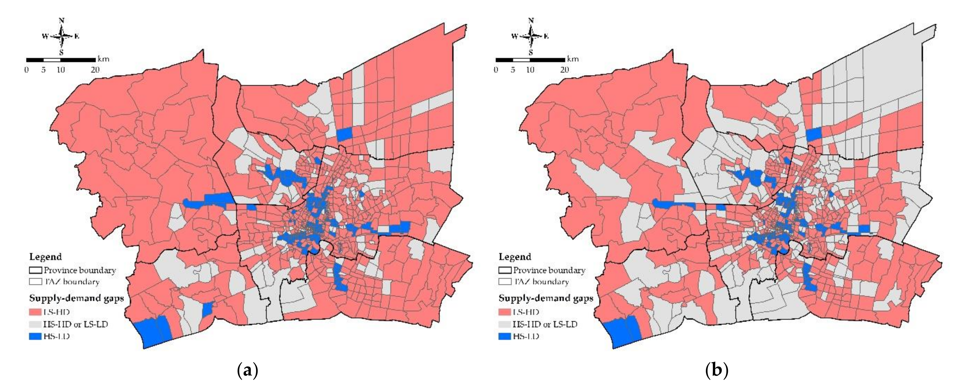
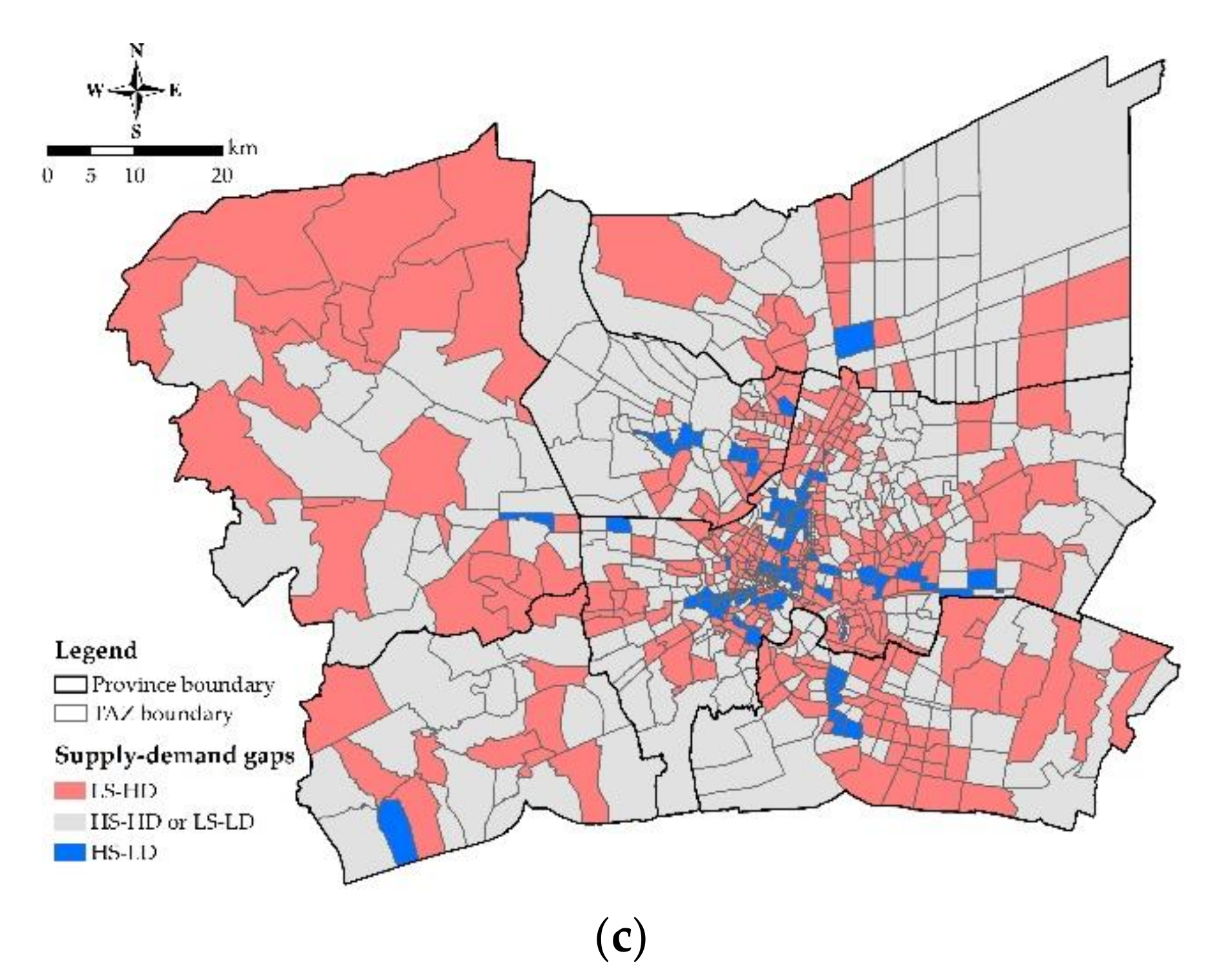
5.4. Supply–Demand Gaps
- High gap areas with high public transport supply are mostly the business area along the metro lines which has many office buildings and large popular shopping centers. These areas have commuting demand for work purposes as well as other activities such as school, hospital, shopping, as well as government services. On the other hand, high gap areas with low public transport supply are mostly in residential areas, including non-business areas such as agricultural areas, livestock areas, and countryside.
- Overall supply–demand gaps show that most of the population in BMR are placed under the LS-HD area. Moreover, most of the low-income households (<30,000) in vicinities were found in these LS-HD categories but in Bangkok and Nonthaburi were found in the middle-income household (30,000–50,000). The second proportion of the population in BMR was placed under LS-LD or HS-HD area. Lastly, the very small size of the population was placed under the HS-LD area.
- The results display that it has more than 50% of the population proportion, which has big gaps between supply–demand for public transport. The largest gaps between the supply–demand were found in Nakhon Pathom province followed by Samut Prakan, Pathum Thani, and Samut Sakhon, which accounts for the population proportion about 88%, 72%, 71%, and 69% respectively. Additionally, it was found that the LS-HD area occurs mostly in the surrounding provinces with low-income households’ distribution except for Bangkok and Nonthaburi, where the LS-HD area was found in middle-income households more than low-income household.
- The results also show that HS-HD or LS-LD area was indicated about 20% to 40% of the population in BMR. Nonthaburi province has the largest number of populations placed under the HS-HD or LS-LD area, and accounted for about 40% of the population followed by Samut Prakan, Pathum Thani, and Bangkok, which accounted for about 27%, 24%, and 20% of the population proportion, respectively. For Bangkok and Nonthaburi, HS-HD or LS-LD area was mostly distributed in middle-income households’ area, whereas the remaining provinces was distributed in low-income households’ area.
- Only three provinces appeared in the HS-LD area for public transport more than 10% of the population proportion; which are Bangkok, Nonthaburi, and Samut Prakan. Bangkok has the most population distribution placed under the HS-LD area for public transportation, and accounted for about 14% of the total population. Moreover, it occurred in middle-income and high-income household’s distribution areas. For Pathum Thani, Nakhon Pathom, and Samut Sakhon provinces, less than 5% of population distribution area were indicated as an HS-LD area.
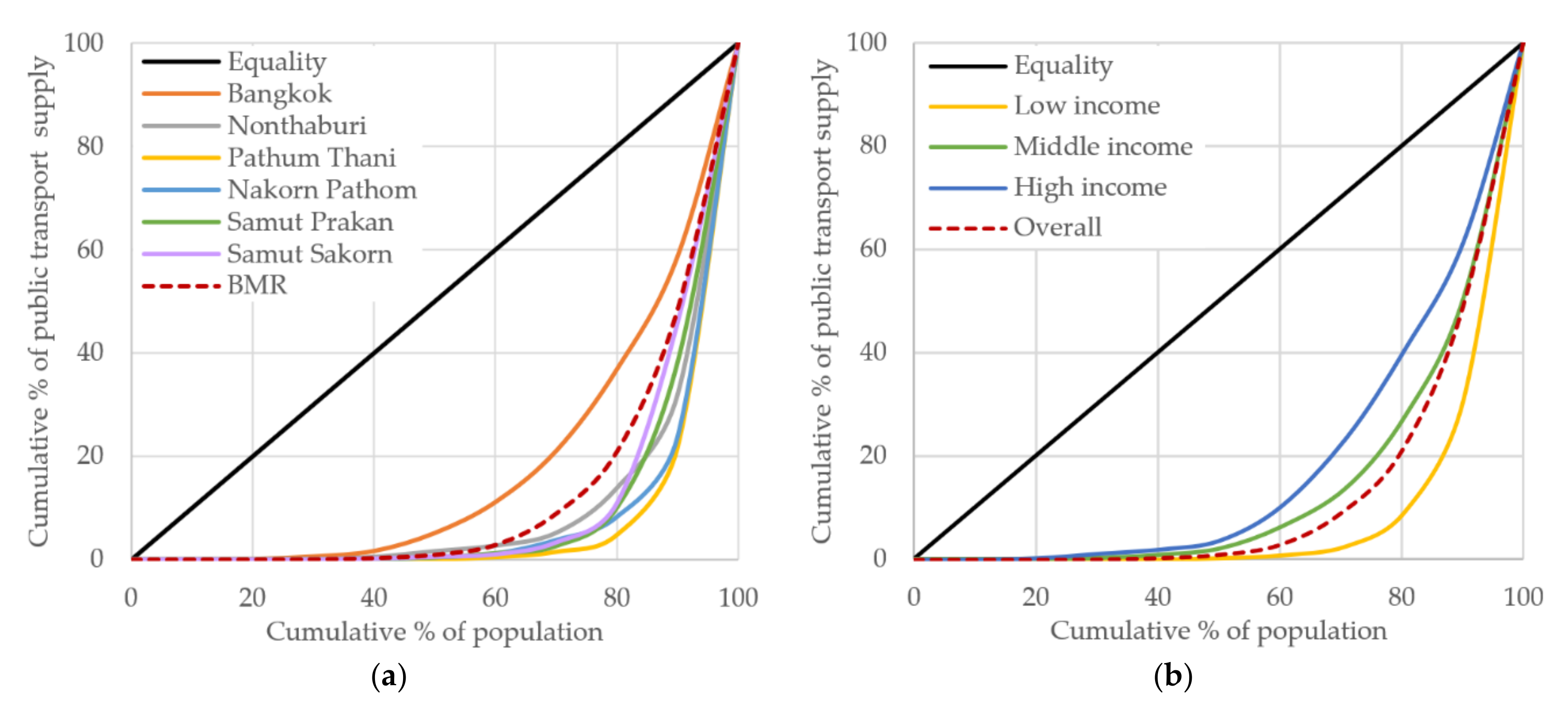
5.5. Lorenz Curves and Gini Coefficients
6. Discussion
7. Conclusions
Author Contributions
Funding
Acknowledgments
Conflicts of Interest
References
- Hideo, N.; Mikiharu, A.; Yoshikuni, K.; Hideo, N. Overview of Urban Transport and the Environment. In Urban Transport and the Environment; Emerald Group Publishing Limited: Bingley, UK, 2004; pp. 11–36. [Google Scholar]
- Daniel, S.; Shinya, H.; Akira, O.; Makoto, O.; Wolfgang, S.; Masaharu, Y. Environmental Impacts Due to Urban Transport. In Urban Transport and the Environment; Emerald Group Publishing Limited: Bingley, UK, 2004; pp. 99–190. [Google Scholar]
- Nielsen, R.S. Problems and Possible Solutions in Urban Transport Planning in Australia. Aust. J. Public Adm. 1972, 31, 168–174. [Google Scholar] [CrossRef]
- Cao, X.; Chen, H.; Liang, F.; Wang, W. Measurement and Spatial Differentiation Characteristics of Transit Equity: A Case Study of Guangzhou, China. Sustainability 2018, 10, 1069. [Google Scholar] [CrossRef] [Green Version]
- Lope, D.J.; Dolgun, A. Measuring the Inequality of Accessible Trams in Melbourne. J. Transp. Geogr. 2020, 83, 102657. [Google Scholar] [CrossRef]
- Alotaibi, O.; Potoglou, D. Perspectives of Travel Strategies in Light of the New Metro and Bus Networks in Riyadh City, Saudi Arabia. Transp. Plan. Technol. 2017, 40, 4–27. [Google Scholar] [CrossRef] [Green Version]
- Oviedo, D.; Guzman, L.A. Revisiting Accessibility in a Context of Sustainable Transport: Capabilities and Inequalities in Bogota. Sustainability 2020, 12, 4464. [Google Scholar] [CrossRef]
- Tennøy, A.; Tønnesen, A.; Gundersen, F. Effects of Urban Road Capacity Expansion—Experiences from Two Norwegian Cases. Transp. Res. Part D 2019, 69, 90–106. [Google Scholar] [CrossRef]
- Pucher, J.; Korattyswaropam, N.; Mittal, N.; Ittyerah, N. Urban Transport Crisis in India. Transp. Policy 2005, 12, 185–198. [Google Scholar] [CrossRef]
- Gakenheimer, R. Urban Mobility in the Developing World. Transp. Res. Part A 1999, 33, 671–689. [Google Scholar] [CrossRef]
- Tanaboriboon, Y. Bangkok Traffic. IATSS Res. 1993, 17, 14–23. [Google Scholar]
- Vichiensan, V. Dynamics of Urban Structure in Bangkok Based on Employment Cluster and Commuting Pattern. J. East. Asia Soc. Transp. Stud. 2007, 7, 1559–1574. [Google Scholar]
- Pala-En, N.; Manomaiphiboon, K.; Boonyoo, T.; Kokkaew, E.; Pattaramunikul, S.; Nakharin, P. Traffic-Model-Based Emissions for Transportation Sector to Support PM2.5 Management in Bangkok and Its Vicinity: Initial Results. In National Conference on Air Quality in Thailand: PM2.5; Thailand network center on Air Quality Management (TAQM): Bangkok, Thailand, 2019; pp. 80–87. [Google Scholar]
- Rujopakarn, W. Transportation System and Urban Planning in Bangkok. Kasetsart Eng. J. 1992, 17, 51–61. [Google Scholar]
- The Office of Traffic and Transport Policy and Planning. 20 Years’ Thailand Transport System Development Strategy (2017–2036); Minister of Transport: Bangkok, Thailand, 2015. [Google Scholar]
- Office of the National Economic and Social Development Board. The Twelfth National Economic and Social Development Plan (2017–2021); Office of the Prime Minister: Bangkok, Thailand, 2017. [Google Scholar]
- SEA Consult Engineering Co.; PSK Consulttants Co.; Thammasat University Research and Consultancy Institute; Plan Pro Corp. Thailand Transport and Traffic Database for Competitiveness Assessment; Ministry of Transport: Bangkok, Thailand, 2016. [Google Scholar]
- Pojani, D.; Stead, D. Sustainable Urban Transport in the Developing World: Beyond Megacities. Sustainability 2015, 7, 7784–7805. [Google Scholar] [CrossRef] [Green Version]
- Vichiensan, V. Urban Mobility and Employment Accessibility in Bangkok: Present and Future; Cooperation for Urban Mobility in the Developing World (CODATU): Dakar, Senegal, 2008. [Google Scholar]
- The Office of Traffic and Transport Policy and Planning. Travel of the People of Bangkok, Vicinity and Continuous Areas; Minister of Transport: Bangkok, Thailand, 2018. [Google Scholar]
- Kii, M.; Hanaoka, S. Comparison of Sustainability between Private and Public Transport Consideration Urban Structure. IATSS Res. 2003, 27, 6–15. [Google Scholar] [CrossRef] [Green Version]
- Permana, A.S.; Petchsasithon, A. Assessing the Seamlessness of Bangkok Metropolitan Public Transport by Using Modified Quantitative Gap Analysis. Int. J. Built Environ. Sustain. 2020, 7, 81–97. [Google Scholar] [CrossRef]
- Macioszek, E.; Świerk, P.; Kurek, A. The Bike-Sharing System as an Element of Enhancing Sustainable Mobility—A Case Study Based on a City in Poland. Sustainability 2020, 12, 3285. [Google Scholar] [CrossRef] [Green Version]
- Nikiforiadis, A.; Ayfantopoulou, G.; Stamelou, A. Assessing the Impact of COVID-19 on Bike-Sharing Usage: The Case of Thessaloniki, Greece. Sustainability 2020, 12, 8215. [Google Scholar] [CrossRef]
- Politis, I.; Fyrogenis, I.; Papadopoulos, E.; Nikolaidou, A.; Verani, E. Shifting to Shared Wheels: Factors Affecting Dockless Bike-Sharing Choice for Short and Long Trips. Sustainability 2020, 12, 8205. [Google Scholar] [CrossRef]
- Ibrahim, A.N.H.; Borhan, M.N.; Rahmat, R.A.O.K. Understanding Users’ Intention to Use Park-and-Ride Facilities in Malaysia: The Role of Trust as a Novel Construct in the Theory of Planned Behaviour. Sustainability 2020, 12, 2484. [Google Scholar] [CrossRef] [Green Version]
- MacIoszek, E.; Kurek, A. The Use of a Park and Ride System a Case Study Based on the City of Cracow (Poland). Energies 2020, 13, 3473. [Google Scholar] [CrossRef]
- Pomlaktong, N.; Jongwilaiwan, R.; Theerawattanakul, P.; Pholpanich, R. Road Transport in Thailand. In Priorities and Pathways in Services Reform—Part II Political Economy Studies; Findlay, C., Ed.; World Scientific Publishing Company: Singapore, 2013; pp. 227–243. [Google Scholar]
- Currie, G. Quantifying Spatial Gaps in Public Transport Supply Based on Social Needs. J. Transp. Geogr. 2010, 18, 31–41. [Google Scholar] [CrossRef]
- Delbosc, A.; Currie, G. Using Lorenz Curves to Assess Public Transport Equity. J. Transp. Geogr. 2011, 19, 1252–1259. [Google Scholar] [CrossRef]
- Dobranskyte-Niskota, A.; Perujo, A.; Pregl, M. Indicators to Assess Sustainability of Transport Activities; Joint Research Centre Institute for Environment and Sustainability Contact: Luxembourg, 2007. [Google Scholar]
- The Vancouver Conference. Towards Sustainable Transportation. In Towards Sustainable Transportation; The Secretary-General, the Government of Canada: Vancouver, BC, Canada, 1996. [Google Scholar]
- Litman, T. Well Measured: Developing Indicators for Sustainable and Livable Transport Planning; Victoria Transport Policy Institute: Victoria, BC, Canada, 2016; pp. 10–15. [Google Scholar]
- Meyer, M. Measuring that Which Cannot Be Measured—At Least According to Conventional Wisdom. In Performance Measures to Improve Transportation Systems and Agency Operations; National Academies Press: Washington, DC, USA, 2001; pp. 105–125. [Google Scholar]
- Kittelson & Associates; Urbitran; LKC Consulting Service; MORPACE International; Queensland University of Technology; Nakanishim, Y. A Guidebook for Developing a Transit Performance-Measurement System; Transportation Research Board: Washington, DC, USA, 2003. [Google Scholar]
- Dhingra, C. Measuring Public Transport Performance—Lessons for Developing Cities; Deutsche Gesellschaft für Internationale Zusammenarbeit (GIZ): Berlin/Heidelberg, Germany, 2011. [Google Scholar]
- Eboli, L.; Mazzulla, G. Performance Indicators for an Objective Measure of Public Transport Service Quality. Eur. Transp. 2012, 51, 1–21. [Google Scholar]
- D’Arcier, B.F. Measuring the Performance of Urban Public Transport in Relation to Public Policy Objectives. Res. Transp. Econ. 2014, 48, 67–76. [Google Scholar]
- Litman, B.T. Measuring Transportation: Traffic, Mobility and Accessibility. Inst. Transp. Eng. 2011, 73, 28–32. [Google Scholar]
- Moseley, M.J. Accessibility: The Rural Challenge; University Paperbacks: Methuen, MA, USA, 1979. [Google Scholar]
- Wu, B.M.; Hine, J.P. A PTAL Approach to Measuring Changes in Bus Service Accessibility. Transp. Policy 2003, 10, 307–320. [Google Scholar] [CrossRef]
- Hine, J.; Mitchell, F. Transport Disadvantage and Social Exclusion: Exclusionary Mechanisms in Transport in Urban Scotland; Routledge: Abingdon, UK, 2017. [Google Scholar]
- Currie, G. Gap Analysis of Public Transport Needs Measuring Spatial Distribution of Public Transport Needs and Identifying Gaps in the Quality of Public Transport Provision. J. Transp. Res. Board 2004, 1895, 137–146. [Google Scholar] [CrossRef]
- De Palma, A.; Lindsey, R. Transportation: Supply and Congestion; Pergamon: Oxford, UK, 2001; pp. 5882–15888. [Google Scholar]
- Jiao, J.; Dillivan, M. Transit Deserts: The Gap between Demand and Supply. J. Public Transp. 2013, 16, 23–39. [Google Scholar] [CrossRef] [Green Version]
- Fransen, K.; Neutens, T.; Farber, S.; De Maeyer, P.; Deruyter, G.; Witlox, F. Identifying Public Transport Gaps Using Time-Dependent Accessibility Levels. J. Transp. Geogr. 2015, 48, 176–187. [Google Scholar] [CrossRef] [Green Version]
- Chen, Y.; Bouferguene, A.; Xian, H.; Liu, H.; Shen, Y. Spatial Gaps in Urban Public Transport Supply and Demand from the Perspective of Sustainability. J. Clean. Prod. 2018, 195, 1237–1248. [Google Scholar] [CrossRef]
- Litman, T. Evaluating Transportation Equity. World Transp. Policy Pract. 2002, 8, 50–65. [Google Scholar]
- Guzman, L.A.; Oviedo, D. Accessibility, Affordability and Equity: Assessing ‘Pro-Poor’ Public Transport Subsidies in Bogotá. Transp. Policy 2018, 68, 37–51. [Google Scholar] [CrossRef]
- Lee, S.; Mark, S.; Lee, K. Journal of King Saud University—Engineering Sciences Original Article A Gini Coefficient Based Evaluation on the Reliability of Travel Time Forecasting. J. King Saud Univ. Eng. Sci. 2019, 31, 314–319. [Google Scholar]
- Prasertsubpakij, D.; Nitivattananon, V. Evaluating Accessibility to Bangkok Metro Systems Using Multi-Dimensional Criteria across User Groups. IATSS Res. 2012, 36, 56–65. [Google Scholar] [CrossRef] [Green Version]
- Openshaw, S. The Modifiable Areal Unit Problem; Geo-Books: Norwich, UK, 1983. [Google Scholar]
- Armstrong-Wright, A.; Thiriez, S. Bus Services—Reducing Costs, Raising Standards; World Bank: Washington, DC, USA, 1987; p. 56. [Google Scholar]
- Yang, R.; Liu, Y.; Liu, Y.; Liu, H.; Gan, W. Comprehensive Public Transport Service Accessibility Index—A New Approach Based on Degree Centrality and Gravity Model. Sustainability 2019, 11, 5634. [Google Scholar] [CrossRef] [Green Version]
- Currie, G.; Wallis, I. Determining Priorities for Passenger Transport Funding: The Needs Assessment Approach. Australas. Transp. Res. Forum. 1992, 17, 55–67. [Google Scholar]
- Kittelson & Associates; KFH Groups; Parsons Brinckerhoff Quade & Douglass; Zaworski, K.H. Transit Capacity and Quality of Service Manual, Second Ed., 2nd ed.; Transportation Research Board: Washington, DC, USA, 2003. [Google Scholar]
- Chalermpong, S.; Wibowo, S.S. Transit Station Access Trips and Factors Affecting Propensity to Walk to Transit Stations in Bangkok, Thailand. J. East. Asia Soc. Transp. Stud. 2007, 7, 1806–1819. [Google Scholar]
- McNally, M.G. The Four Step Model. Handb. Transp. Model. 2000, 1, 35–41. [Google Scholar]
- McNally, M.G. The Four-Step Model. In Handbook of Transport Modelling; Hensher, D.A., Button, K.J., Eds.; Emerald Group Publishing Limited: Bingley, UK, 2007; Volume 1, pp. 35–53. [Google Scholar]
- Lorenz, M.O. Methods of Measuring the Concentration of Wealth. Publ. Am. Stat. Assoc. 1905, 9, 209–219. [Google Scholar] [CrossRef]
- Chen, Y.; Tan, H.; Berardi, U. Energy & Buildings a Data-Driven Approach for Building Energy Benchmarking Using the Lorenz Curve. Energy Build. 2018, 169, 319–331. [Google Scholar]
- Groves-Kirkby, C.J.; Denman, A.R.; Phillips, P.S. Lorenz Curve and Gini Coefficient: Novel Tools for Analysing Seasonal Variation of Environmental Radon Gas. J. Environ. Manage. 2009, 90, 2480–2487. [Google Scholar] [CrossRef]
- Pavkova, K.; Currie, G.; Delbosc, A.; Sarvi, M. Selecting Tram Links for Priority Treatments—The Lorenz Curve Approach. J. Transp. Geogr. 2016, 55, 101–109. [Google Scholar] [CrossRef]
- Yang, A.; Fan, H.; Jing, N.; Sun, Y.; Zipf, A. Temporal Analysis on Contribution Inequality in OpenStreetMap: A Comparative Study for Four Countries. Int. J. Geo-Inf. 2016, 5, 5. [Google Scholar] [CrossRef]
- Groot, L. Carbon Lorenz Curves. Resour. Energy Econ. 2010, 32, 45–64. [Google Scholar] [CrossRef]
- Gini, C.W. Variability and Mutability, Contribution to the Study of Statistical Distributions and Relations; Studi Economico-Giuridici Della R. Universita de Cagliari; Unione Arti Grafiche: Cagliari, Italy, 1912. [Google Scholar]
- Ranjit, S.; Witayangkurn, A.; Nagai, M.; Shibasaki, R. Agent-Based Modeling of Taxi Behavior Simulation with Probe Vehicle Data. ISPRS Int. J. Geo-Inf. 2018, 7, 177. [Google Scholar] [CrossRef] [Green Version]
- Grubler, A. The Transportation Sector: Growing Demand and Emissions. Pac. Asian J. Energy 1994, 3, 179–199. [Google Scholar]
- Peungnumsai, A.; Witayangkurn, A.; Nagai, M.; Miyazaki, H. A Taxi Zoning Analysis Using Large-Scale Probe Data: A Case Study for Metropolitan Bangkok. Rev. Socionetwork Strateg. 2018, 12, 21–45. [Google Scholar] [CrossRef]
- Institute for Research and Academic Service (IRAS), A.U. Bangkok Media and Broadcasting Online. Available online: https://www.pptvhd36.com/news/%E0%B8%9B%E0%B8%A3%E0%B8%B0%E0%B9%80%E0%B8%94%E0%B9%87%E0%B8%99%E0%B8%A3%E0%B9%89%E0%B8%AD%E0%B8%99/80498 (accessed on 9 August 2020).
- Peungnumsai, A.; Witayangkurn, A.; Nagai, M.; Arai, A.; Ranjit, S.; Ghimire, B.R. Bangkok Taxi Service Behavior Analysis Using Taxi Probe Data and Questionnaire Survey. In Proceedings of the 4th Multidisciplinary International Social Networks Conference; Association for Computing Machinery: New York, NY, USA, 2017; pp. 1–8. [Google Scholar]
- TomTom International BV. TomTom Traffic Index: Global Traffic Congestion Up as Bengaluru Takes Crown of ‘World’s Most Traffic Congested City; TomTom N.V.: Amsterdam, The Netherlands, 2020; pp. 1–4. [Google Scholar]
- Hicks, W. Bangkok Post Web Page. Available online: https://www.bangkokpost.com/business/1905450/outbreak-jump-starts-work-from-home (accessed on 9 August 2020).
- Saxena, S. Asian Development Blog. Available online: https://blogs.adb.org/blog/work-home-beat-traffic (accessed on 9 August 2020).


| Dataset | Data Type | Data Description | Number of Transport Routes/Stations/Vehicles | Data Source |
|---|---|---|---|---|
| Heavy rails | Points and lines | Consists of sky trains and subways; BTS 1, MRTA 2, and ARL 3 | 111 stations 5 lines | OTP |
| Buses | Points and lines | Comprise of non-AC buses, AC buses, and Bus Rapid Transit (BRT) | 4773 bus stops 2715 buses 197 routes | Bangkok Mass Transit Authority (BMTA) Bangkok Metropolitan Administration (BMA) |
| Vans | Points | Contain the main vans stations in Bangkok and vicinities | 24 stations | Open Street Map (OSM) |
| Taxis | Points | Stay points of taxis obtaining from taxi probe data | 2678 taxis | Taxi stay point analyzed by Ranjit [67] |
| Boats | Points and lines | Consists of boat lines and piers along Chao Phraya river and Saen Saep canal | 69 piers 6 lines (Chao Phraya river) 2 lines (Saen Saep canal) | Marine Department |
| Trains | Points and lines | Intercity trains on the Northern, North Eastern, and Southern Train Lines stop. | 69 stations 5 routes | State Railway of Thailand (SRT) OSM |
| Dataset | Section Name | Survey Information | Boundary | Number of Zones | Data Source |
|---|---|---|---|---|---|
| Household travel demand survey | Household information | House type, number of a family member, number of own vehicles in the household | TDS | 1607 zones | OTP, MOT |
| Personal Travel Details (Age between 4 to 80) | Vehicle type, trip information, trip number, trip purpose, origin, destination, travel mode | ||||
| Population Density | - | Number of people in each area | Admin | 477 zones | BORA |
| Income | - | Average household income | TAZ | 846 zones | OTP, MOT |
| Major Dimension | Minor Dimension | Current Indicators | Proposed Indicators |
|---|---|---|---|
| Supply/ Availability/ Capacity | Availability | The density of the public transit network The density of transit station | Number of public transport mode availability The proportion of area covered by public transport walking catchment |
| Capacity | - | Number of service capacity The proportion of the number of service capacity and population | |
| Supply | Public transport supply index | ||
| Equity * | Service equity | - | Public transport supply–demand gap Gini coefficients |
| Descriptor | Bangkok | Vicinities | Total | ||||
|---|---|---|---|---|---|---|---|
| Nonthaburi | Pathum Thani | Nakhon Pathom | Samut Prakan | Samut Sakhon | |||
| Number of TAZs | 546 | 81 | 58 | 41 | 93 | 27 | 846 |
| Total area (sq. km) | 1571.02 | 637.46 | 1512.39 | 2149.01 | 999.97 | 863.92 | 7733.77 |
| Average area of TAZ (sq. km) | 2.88 | 7.87 | 26.08 | 52.41 | 10.75 | 32.00 | 9.14 |
| Number of transport stops | |||||||
| Heavy rail (stations) | 88 | 13 | 0 | 0 | 10 | 0 | 111 |
| Buses (stops) | 3720 | 319 | 170 | 143 | 301 | 121 | 4774 |
| Vans (stops) | 11 | 5 | 2 | 2 | 2 | 2 | 24 |
| Taxis (stay points) | 1665 | 312 | 192 | 43 | 387 | 78 | 2677 |
| Boats (Piers) | 58 | 11 | 0 | 0 | 0 | 0 | 69 |
| Trains (stations) | 37 | 1 | 2 | 10 | 0 | 17 | 67 |
| Total number of transport stops | 5579 | 661 | 366 | 198 | 700 | 218 | 7722 |
| % number of transport stops | 72.25% | 8.56% | 4.74% | 2.56% | 9.07% | 2.82% | 100.00% |
| Total public transport service area (sq. km) | 579.50 | 84.63 | 49.33 | 83.08 | 76.61 | 102.57 | 975.72 |
| % Public transport service area | 36.89% | 13.28% | 3.26% | 3.87% | 7.66% | 11.87% | 12.62% |
| Total number of service capacity (number of trips) | 1,650,871 | 186,803 | 79,174 | 72,813 | 181,172 | 48,544 | 2,219,377 |
| % Number of service capacity | 74.38% | 8.42% | 3.57% | 3.28% | 8.16% | 2.19% | 100.00% |
| BMR | NSIP Categories | Total | |||||||
|---|---|---|---|---|---|---|---|---|---|
| No Supply | <20 | 21–40 | 41–60 | 61–80 | 81–100 | >100 | |||
| Bangkok | Number of TAZs | 87 | 157 | 63 | 49 | 43 | 25 | 122 | 546 |
| Population | 1,651,202 | 2,171,232 | 522,294 | 381,405 | 202,697 | 126,004 | 385,120 | 5,439,954 | |
| % Population | 30.35 | 39.91 | 9.60 | 7.01 | 3.73 | 2.32 | 7.08 | 100.00 | |
| Nontha-buri | Number of TAZs | 36 | 30 | 6 | 3 | 3 | 1 | 2 | 81 |
| Population | 669,900 | 437,442 | 73,397 | 26,633 | 29,644 | 6222 | 11,898 | 1,255,136 | |
| % Population | 53.37 | 34.85 | 5.85 | 2.12 | 2.36 | 0.50 | 0.95 | 100.00 | |
| Pathum Thani | Number of TAZs | 51 | 6 | 1 | 0 | 0 | 0 | 0 | 58 |
| Population | 1,028,639 | 142,870 | 56,479 | 0 | 0 | 0 | 0 | 1,227,988 | |
| % Population | 83.77 | 11.63 | 4.60 | 0.00% | 0.00% | 0.00% | 0.00 | 100.00 | |
| Nakhon Pathom | Number of TAZs | 30 | 8 | 1 | 0 | 1 | 0 | 1 | 41 |
| Population | 831,732 | 161,292 | 6152 | 0 | 5652 | 0 | 3001 | 1,007,829 | |
| % Population | 82.53 | 16.00 | 0.61 | 0.00 | 0.56 | 0.00 | 0.30 | 100.00 | |
| Samut Prakan | Number of TAZs | 65 | 15 | 5 | 5 | 2 | 1 | 0 | 93 |
| Population | 926,489 | 309,366 | 106,047 | 72,559 | 15,824 | 7202 | 0 | 1,437,487 | |
| % Population | 64.45 | 21.52 | 7.38 | 5.05 | 1.10 | 0.50 | 0.00 | 100.00 | |
| Samut Sakhon | Number of TAZs | 17 | 8 | 2 | 0 | 0 | 0 | 0 | 27 |
| Population | 502,842 | 177,936 | 11,291 | 0 | 0 | 0 | 0 | 692,069 | |
| % Population | 72.66 | 25.71 | 1.63 | 0.00 | 0.00 | 0.00 | 0.00 | 100.00 | |
| BMR | NDIP Categories | Total | ||||||
|---|---|---|---|---|---|---|---|---|
| <20 | 21–40 | 41–60 | 61–80 | 81–100 | >100 | |||
| Bangkok | Number of TAZs | 139 | 111 | 76 | 61 | 28 | 131 | 546 |
| Population | 2,456,083 | 1,299,956 | 700,245 | 376,007 | 188,326 | 419,337 | 5,439,954 | |
| % Population | 45.15 | 23.90 | 12.87 | 6.91 | 3.46 | 7.71 | 100.00 | |
| Nontha-buri | Number of TAZs | 49 | 21 | 2 | 2 | 4 | 3 | 81 |
| Population | 872,595 | 219,439 | 37,871 | 42,994 | 62,009 | 20,228 | 1,255,136 | |
| % Population | 69.52 | 17.48 | 3.02 | 3.43 | 4.94 | 1.61 | 100.00 | |
| Pathum Thani | Number of TAZs | 45 | 6 | 4 | 2 | 0 | 1 | 58 |
| Population | 955,556 | 148,011 | 72,481 | 27,860 | 0 | 24,080 | 1,227,988 | |
| % Population | 77.82 | 12.05 | 5.90 | 2.27 | 0.00 | 1.96 | 100.00 | |
| Nakhon Pathom | Number of TAZs | 23 | 11 | 4 | 0 | 0 | 3 | 41 |
| Population | 628,471 | 283,544 | 59,650 | 0 | 0 | 36,164 | 1,007,829 | |
| % Population | 62.36 | 28.13 | 5.92 | 0.00 | 0.00 | 3.59 | 100.00 | |
| Samut Prakan | Number of TAZs | 49 | 37 | 4 | 1 | 0 | 2 | 93 |
| Population | 775,237 | 599,066 | 44,224 | 732 | 0 | 18,228 | 1,437,487 | |
| % Population | 53.93 | 41.67 | 3.08 | 0.05 | 0.00 | 1.27 | 100.00 | |
| Samut Sakhon | Number of TAZs | 19 | 7 | 0 | 1 | 0 | 0 | 27 |
| Population | 463,180 | 183,298 | 0 | 45,591 | 0 | 0 | 692,069 | |
| % Population | 66.93 | 26.48 | 0.00 | 6.59 | 0.00 | 0.00 | 100.00 | |
| Regions | Supply–Demand Gaps Categories (10% Threshold) | |||||||||
|---|---|---|---|---|---|---|---|---|---|---|
| LS-HD | LS-LD or HS-HD | HS-LD | Sum Pop (%) | |||||||
| TAZs | Pop | %Pop | TAZs | Pop | %Pop | TAZs | Pop | %Pop | ||
| Bangkok | ||||||||||
| <30,000 | 61 | 625,729 | 11.50 | 10 | 128,567 | 2.36 | 17 | 80,939 | 1.49 | 15.35 |
| 30,000–50,000 | 213 | 2,506,162 | 46.70 | 42 | 783,282 | 14.40 | 83 | 576,092 | 10.59 | 71.06 |
| >50,000 | 64 | 438,670 | 8.07 | 11 | 177,333 | 3.26 | 45 | 123,180 | 2.26 | 13.59 |
| Total | 338 | 3,570,561 | 65.64 | 63 | 1,089,182 | 20.02 | 145 | 780,211 | 14.34 | 100.00 |
| Nonthaburi | ||||||||||
| <30,000 | 4 | 56,113 | 4.47 | 3 | 68,661 | 5.47 | 16 | 152,300 | 12.13 | 22.07 |
| 30,000–50,000 | 41 | 536,390 | 42.74 | 14 | 346,793 | 27.63 | 0 | 0 | 0 | 70.37 |
| >50,000 | 2 | 46,630 | 3.72 | 1 | 48,249 | 3.84 | 0 | 0 | 0 | 7.56 |
| Total | 47 | 639,133 | 50.93 | 18 | 463,703 | 39.94 | 16 | 152,300 | 12.13 | 100.00 |
| Pathum Thani | ||||||||||
| <30,000 | 32 | 661,190 | 53.84 | 8 | 190,429 | 15.51 | 1 | 56,479 | 4.60 | 73.95 |
| 30,000–50,000 | 14 | 211,895 | 17.26 | 3 | 107,994 | 8.79 | 0 | 0 | 0 | 26.05 |
| >50,000 | 0 | 0 | 0 | 0 | 0 | 0 | 0 | 0 | 0 | 0 |
| Total | 46 | 873,085 | 71.10 | 11 | 298,423 | 24.30 | 1 | 56,479 | 4.60 | 100.00 |
| Nakhon Pathom | ||||||||||
| <30,000 | 32 | 760,763 | 75.48 | 3 | 88,179 | 8.75 | 3 | 31,934 | 3.17 | 87.40 |
| 30,000–50,000 | 3 | 126,953 | 12.60 | 0 | 0 | 0 | 0 | 0 | 0 | 12.60 |
| >50,000 | 0 | 0 | 0 | 0 | 0 | 0 | 0 | 0 | 0 | 0 |
| Total | 35 | 887,716 | 88.08 | 3 | 88,179 | 8.75 | 3 | 31,934 | 3.17 | 100.00 |
| Samut Prakan | ||||||||||
| <30,000 | 57 | 872,962 | 60.73 | 13 | 239,894 | 16.69 | 11 | 144,255 | 10.03 | 87.45 |
| 30,000–50,000 | 8 | 81,170 | 5.65 | 0 | 0 | 0 | 0 | 0 | 0 | 5.65 |
| >50,000 | 3 | 84,999 | 5.91 | 1 | 14,208 | 0.99 | 0 | 0 | 0 | 6.90 |
| Total | 68 | 1,039,131 | 72.29 | 14 | 254,102 | 17.68 | 11 | 144,255 | 10.03 | 100.00 |
| Samut Sakhon | ||||||||||
| <30,000 | 17 | 478,188 | 69.09 | 7 | 186,565 | 26.96 | 3 | 27,316 | 3.95 | 100.00 |
| 30,000–50,000 | 0 | 0 | 0 | 0 | 0 | 0 | 0 | 0 | 0 | 0 |
| >50,000 | 0 | 0 | 0 | 0 | 0 | 0 | 0 | 0 | 0 | 0 |
| Total | 17 | 478,188 | 69.09 | 7 | 186,565 | 26.96 | 3 | 27,316 | 3.95 | 100.00 |
| Categorized By | Gini Coefficients | |
|---|---|---|
| Province | Bangkok | 0.64 |
| Nonthaburi | 0.81 | |
| Pathum Thani | 0.88 | |
| Nakhon Pathom | 0.86 | |
| Samut Prakan | 0.81 | |
| Samut Sakhon | 0.78 | |
| Household income | Low income | 0.83 |
| Middle income | 0.70 | |
| High income | 0.63 | |
| Overall BMR | 0.75 | |
Publisher’s Note: MDPI stays neutral with regard to jurisdictional claims in published maps and institutional affiliations. |
© 2020 by the authors. Licensee MDPI, Basel, Switzerland. This article is an open access article distributed under the terms and conditions of the Creative Commons Attribution (CC BY) license (http://creativecommons.org/licenses/by/4.0/).
Share and Cite
Peungnumsai, A.; Miyazaki, H.; Witayangkurn, A.; Kim, S.M. A Grid-Based Spatial Analysis for Detecting Supply–Demand Gaps of Public Transports: A Case Study of the Bangkok Metropolitan Region. Sustainability 2020, 12, 10382. https://0-doi-org.brum.beds.ac.uk/10.3390/su122410382
Peungnumsai A, Miyazaki H, Witayangkurn A, Kim SM. A Grid-Based Spatial Analysis for Detecting Supply–Demand Gaps of Public Transports: A Case Study of the Bangkok Metropolitan Region. Sustainability. 2020; 12(24):10382. https://0-doi-org.brum.beds.ac.uk/10.3390/su122410382
Chicago/Turabian StylePeungnumsai, Apantri, Hiroyuki Miyazaki, Apichon Witayangkurn, and Sohee Minsun Kim. 2020. "A Grid-Based Spatial Analysis for Detecting Supply–Demand Gaps of Public Transports: A Case Study of the Bangkok Metropolitan Region" Sustainability 12, no. 24: 10382. https://0-doi-org.brum.beds.ac.uk/10.3390/su122410382