Hydrochemical and Isotopic Applications in the Western Aosta Valley (Italy) for Sustainable Groundwater Management

 , and
, and
Abstract
:1. Introduction
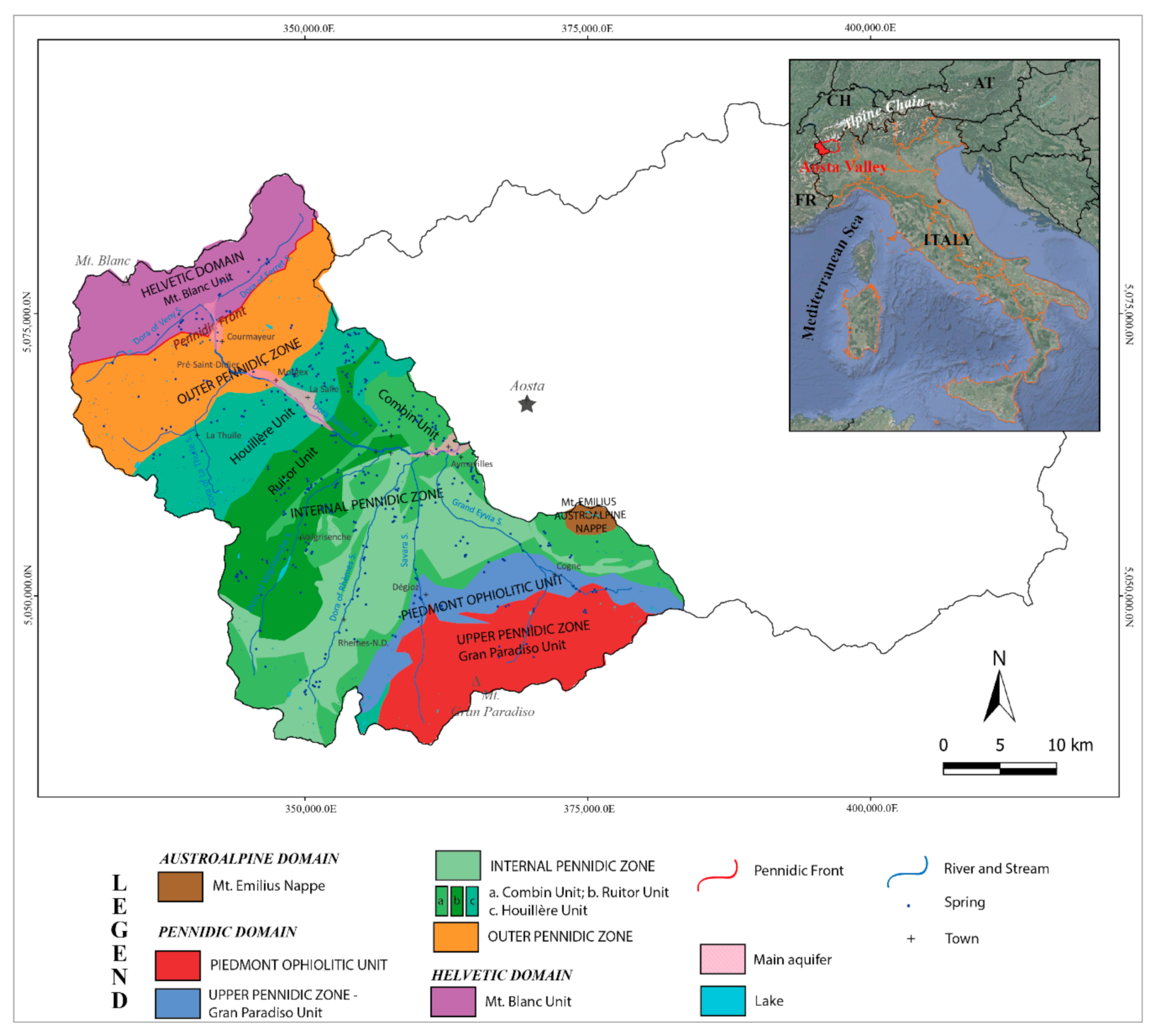
2. Study Area
Previous Isotopic Studies in the Study Area
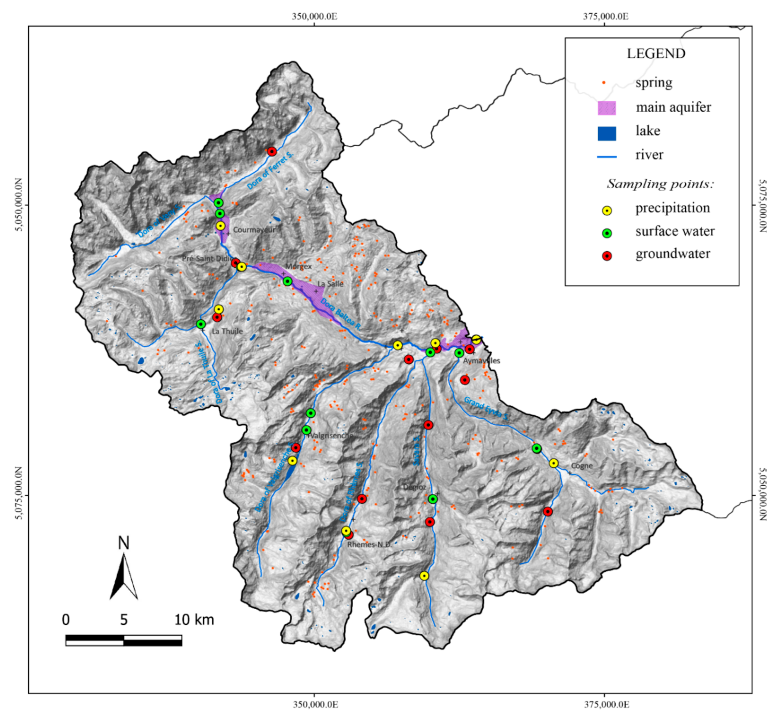
3. Materials and Methods
- -
- One aliquot was collected inside a polyethylene cylindrical bottle with a capacity of 250 mL and a wide neck, screw cap, and sealing disc.One aliquot (the control sample) was collected inside a polyethylene terephthalate (PET) bottle with a capacity of 500 mL.
- -
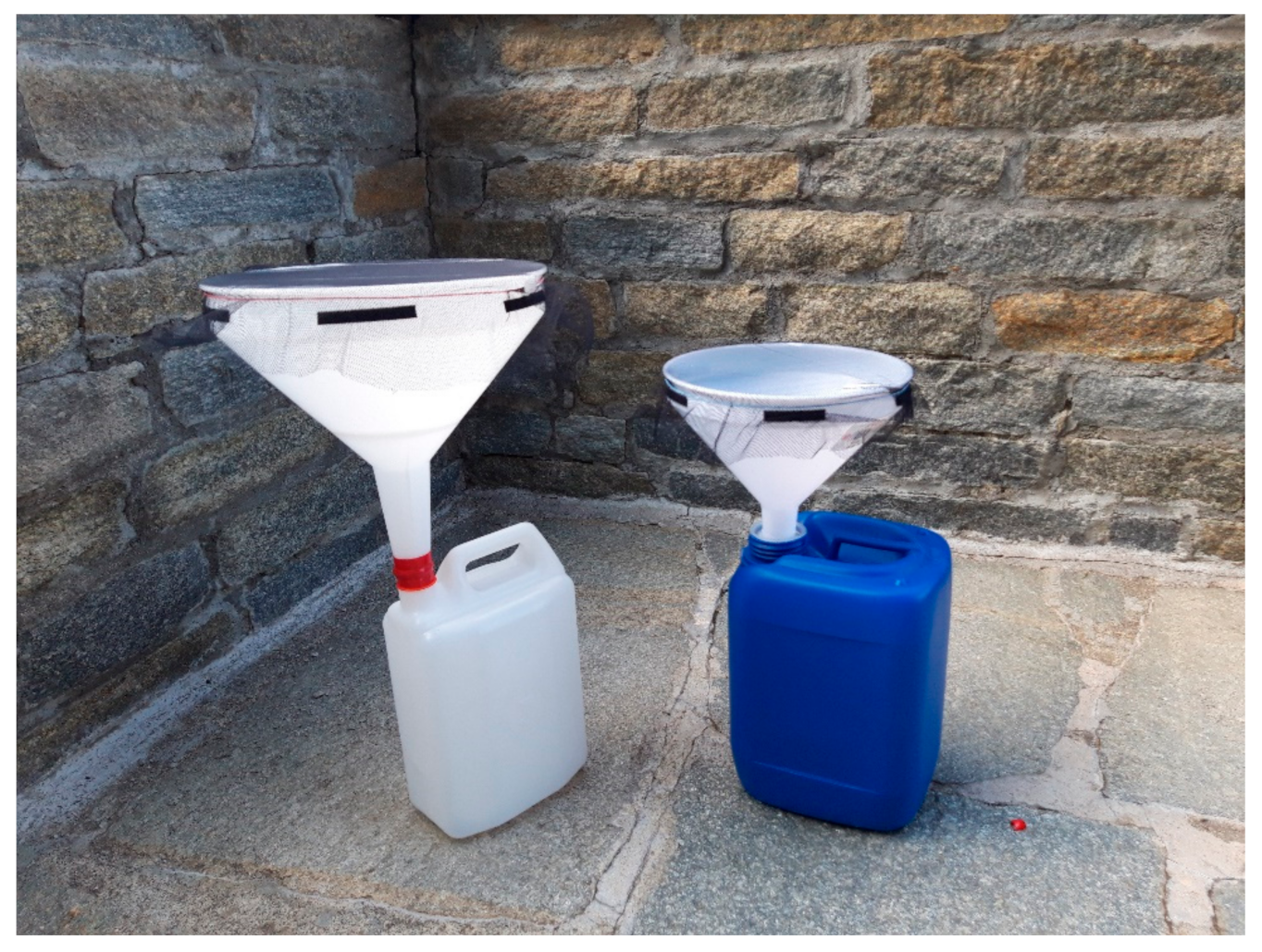
- One aliquot was collected inside a polyethylene cylindrical bottle with a capacity of 250 mL and a wide neck, screw cap, and sealing disc, and one aliquot (the control sample) was collected inside a PET bottle with a capacity of 500 mL; both were collected from precipitation samples taken from the rain gauges without the paraffin oil.
- -
- One aliquot was collected inside a polyethylene cylindrical bottle with a capacity of 250 mL and a wide neck, screw cap, and sealing disc, and one aliquot (the control sample) was collected inside a PET bottle with a capacity of 500 mL; both were collected from a precipitation sample taken from the rain collector with paraffin oil.
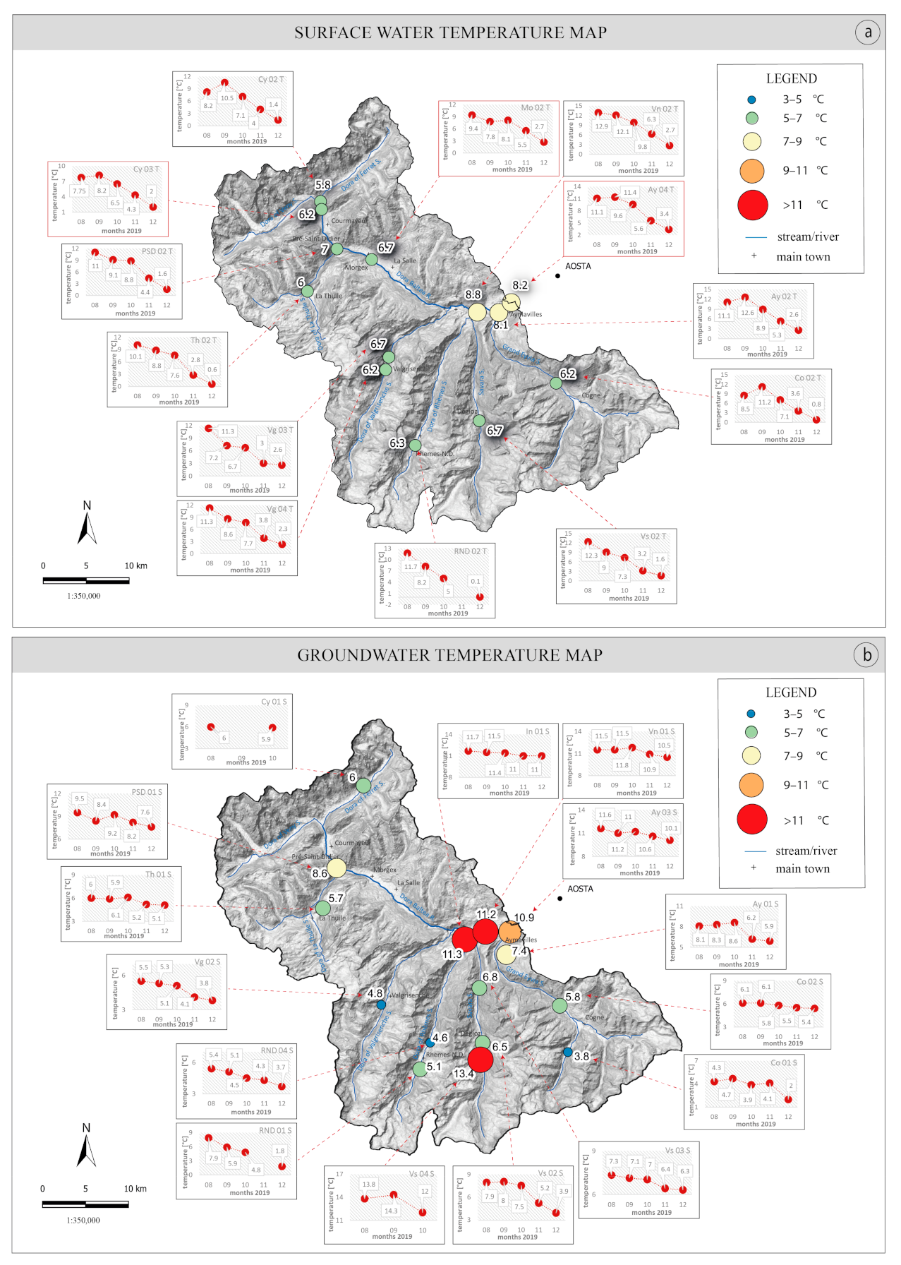
4. Results and Discussion
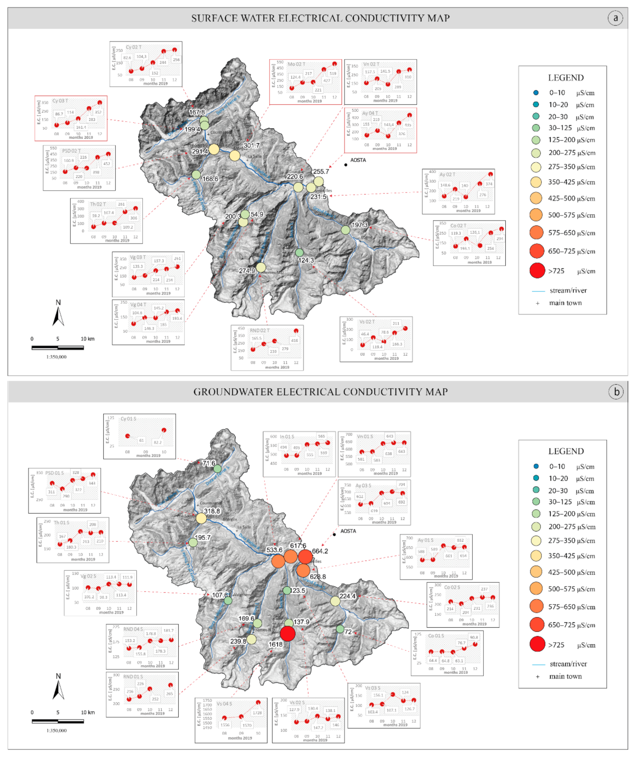
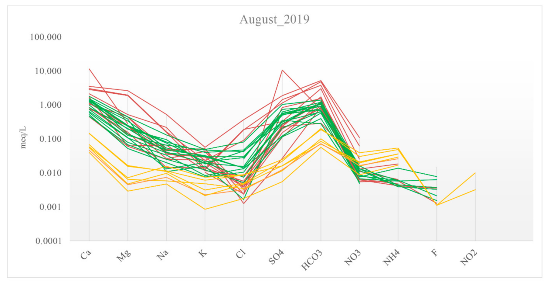
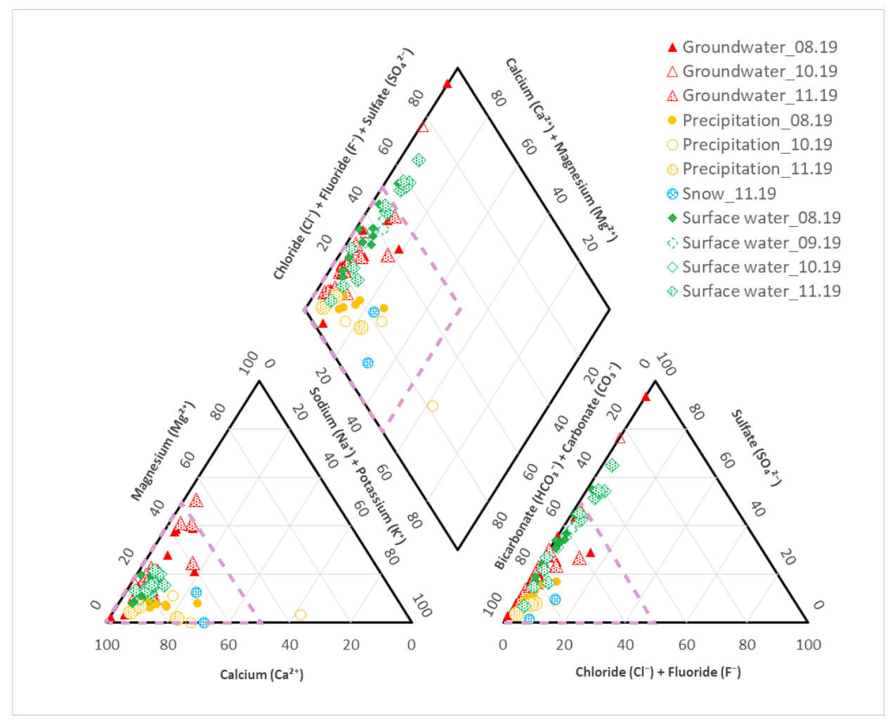
4.1. Chemical Analyses
4.2. Isotopic Analyses
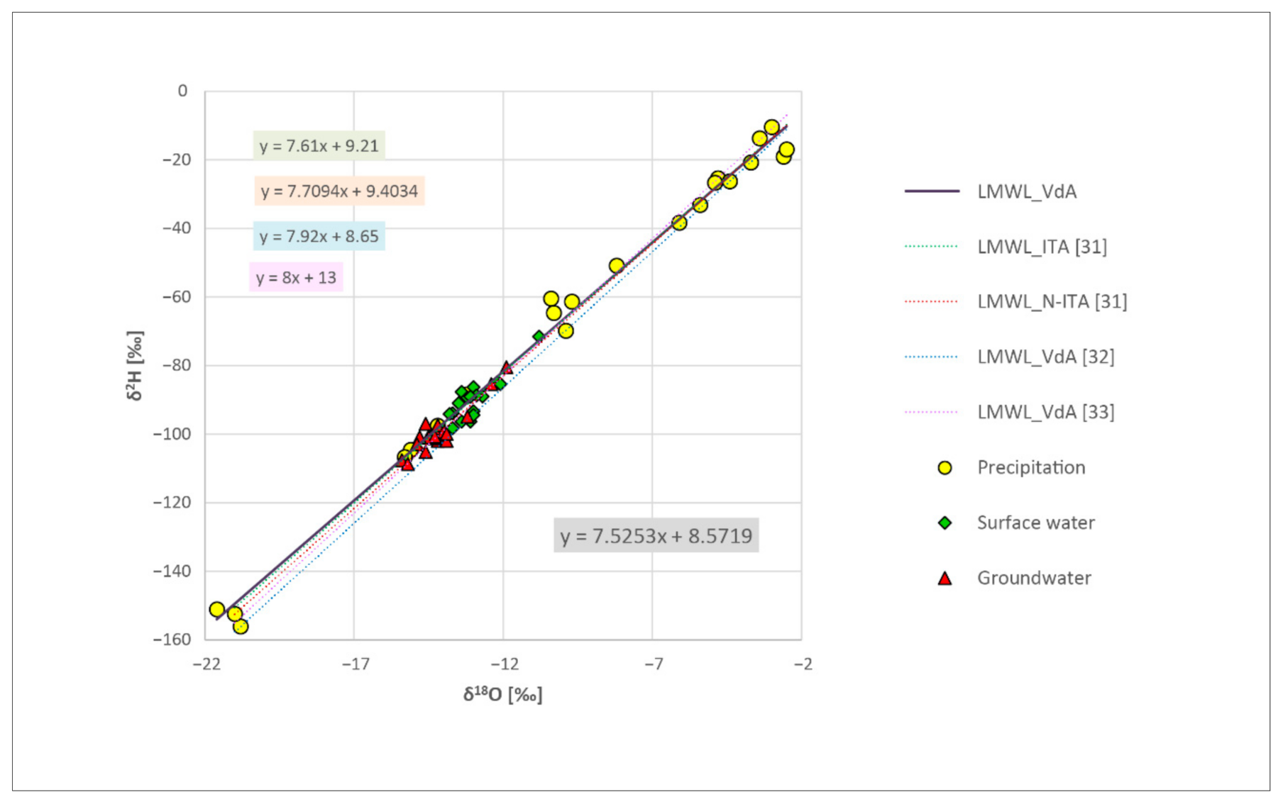
4.2.1. Local Meteoric Water Line (LMWL)
4.2.2. Vertical Isotopic Gradient
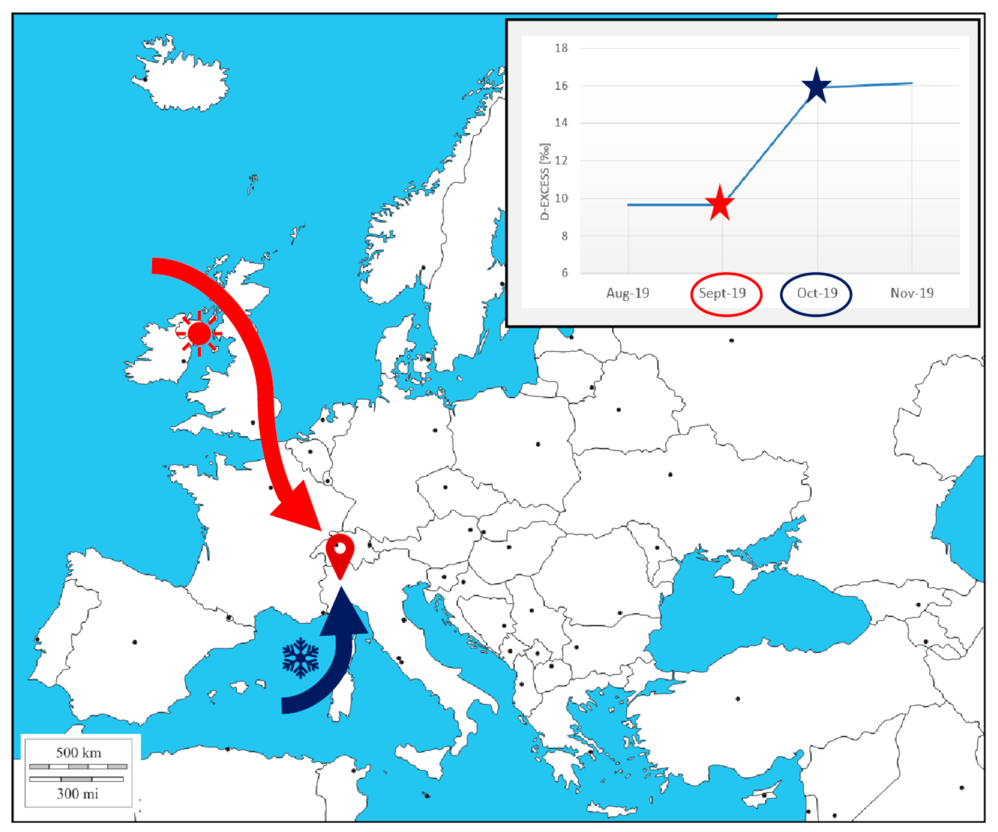
4.2.3. Atlantic and Mediterranean Origin of Precipitation
5. Conclusions and Future Developments
Author Contributions
Funding
Institutional Review Board Statement
Informed Consent Statement
Data Availability Statement
Acknowledgments
Conflicts of Interest
References
- Konikow, L.F.; Kendy, E. Groundwater depletion: A global problem. Hydrogeol. J. 2005, 13, 317–320. [Google Scholar] [CrossRef]
- Taylor, R.G.; Scanlon, B.; Döll, P.; Rodell, M.; Van Beek, R.; Wada, Y.; Longuevergne, L.; Leblanc, M.; Famiglietti, J.S.; Edmunds, M.; et al. Ground water and climate change. Nat. Clim. Chang. 2013, 3, 322–329. [Google Scholar] [CrossRef] [Green Version]
- Gorelick, S.M.; Zheng, C. Global change and the groundwater management challenge. Water Resour. Res. 2015, 51, 3031–3051. [Google Scholar] [CrossRef]
- Lasagna, M.; Mancini, S.; De Luca, D.A. Aquifer protection from overexploitation: Example of actions and mitigation activi-ties used in the Maggiore Valley (Asti Province, NW Italy). Geoingegneria Ambientale e Mineraria 2019, 156, 30–38. [Google Scholar]
- Lasagna, M.; Ducci, D.; Sellerino, M.; Mancini, S.; De Luca, D.A. Meteorological Variability and Groundwater Quality: Examples in Different Hydrogeological Settings. Water 2020, 12, 1297. [Google Scholar] [CrossRef]
- Department of Economic and Social Affairs Sustainable Development. Available online: https://sdgs.un.org/topics/water-and-sanitation (accessed on 15 November 2020).
- Alley, W.M.; Reilly, T.E.; Franke, O.L. Sustainability of Ground-Water Resources; US Geological Survey Circular 1186; USGS: Denver, CO, USA, 1999. [Google Scholar]
- Bhaduri, A.; Bogardi, J.; Siddiqi, A.; Voigt, H.; Vörösmarty, C.; Pahl-Wostl, C.; Bunn, S.E.; Shrivastava, P.; Lawford, R.; Foster, S.; et al. Achieving Sustainable Development Goals from a Water Perspective. Front. Environ Sci. 2016, 4, 64. [Google Scholar] [CrossRef] [Green Version]
- Dzhamalov, R.G.; Zlobina, V.L. Precipitation pollution effect on groundwater hydrochemical regime. Environ. Earth Sci. 1995, 25, 65–68. [Google Scholar] [CrossRef]
- Barbieri, M. Isotopes in Hydrology and Hydrogeology. Water 2019, 11, 291. [Google Scholar] [CrossRef] [Green Version]
- Regione Valle d’Aosta. Available online: http://cf.regione.vda.it/i_giorni_piu.php (accessed on 15 November 2020).
- Polino, R.; Dal Piaz, G.V.; Gosso, G. Tectonic erosion at the Adria margin and accretionary processes for the Cretaceous orogeny of the Alps. Mémoires de la Société Géologique de France (1833) 1990, 156, 345–367. [Google Scholar]
- Lagabrielle, Y.; Lemoine, M. Alpine, Corsican and Apennine ophiolites: The slow-spreading ridge model. Comptes Rendus de l’Académie des Sci. Ser. IIA-Earth Planet. Sci. 1997, 325, 909–920. [Google Scholar] [CrossRef]
- Gasco, I.; Gattiglio, M.; Borghi, A. Review of metamorphic and kinematic data from Internal Crystalline Massifs (Western Alps): PTt paths and exhumation history. J. Geodyn. 2013, 63, 1–19. [Google Scholar] [CrossRef]
- Elter, G. La zona Pennidica dell’Alta e Media Valle D’Aosta e le Unità Limitrofe: Con 22 Figure, 1 tavola fuori testo e 1 Carta Tettonica alla Scala 1: 100 000; Società cooperativa tipografica: Padova, Italy, 1960. [Google Scholar]
- Ellero, A.; Loprieno, A. Nappe stack of Piemonte-Ligurian units south of Aosta Valley: New evidence from Urtier Valley (Western Alps). Geol. J. 2018, 53, 1665–1684. [Google Scholar] [CrossRef]
- Bousquet, R.; Engi, M.; Gosso, G.; Berger, A.; Spalla, M.I.; Zucali, M.; Goffè, B. Explanatory notes to the map: Metamorphic structure of the Alps in Central Alps. Mitt. Österr. Min. Ges. 2004, 149, 41–51. [Google Scholar]
- Forno, M.G.; Comina, C.; Gattiglio, M.; Gianotti, F. Preservation of Quaternary sediments in DSGSD environments: The Mont Fallère case study (Aosta Val-ley, NW Italy). Alp. Mediterr. Quat. 2016, 29, 181–191. [Google Scholar]
- Guillot, F.; Schaltegger, U.; Bertrand, J.-M.; Deloule, E.; Baudin, T. Zircon U–Pb geochronology of Ordovician magmatism in the polycyclic Ruitor Massif (Internal W Alps). Int. J. Earth Sci. 2016, 91, 964–978. [Google Scholar] [CrossRef]
- Bertrand, J.M.; Pidgeon, R.T.; Leterrier, J.; Guillot, F.; Gasquet, G.; Gattiglio, M. SHRIMP and IDTIMS U-Pb zircon ages of the pre-Alpine basement in the Internal Western Alps (Savoy and Piemont). Schweiz. Mineral. Pet-Rographische Mitt. 2000, 80, 225–248. [Google Scholar]
- Elter, G.; Elter, P. Carta Geologica Della Regione del Piccolo S. Bernardo (Versante Italiano); Note Illustrative; Litografia Artistica Cartografica: Firenze, Italy, 1965; p. 53. [Google Scholar]
- Loprieno, A.; Bousquet, R.; Bucher, S.; Ceriani, S.; Torre, F.H.D.; Fügenschuh, B.; Schmid, S.M. The Valais units in Savoy (France): A key area for understanding the palaeogeography and the tectonic evolution of the Western Alps. Int. J. Earth Sci. 2010, 100, 963–992. [Google Scholar] [CrossRef] [Green Version]
- Trumpy, R. Remarques sur la correlation des unites penniques externes entre la Savoie et le Valais et sur l’origine des nappes prealpines. Bsgf Earth Sci. Bull. 1955, 6, 217–231. [Google Scholar] [CrossRef]
- RAVA. Progetti via 992 PRAE: Verifica E Aggiornamento Triennale del Piano Regionale Delle Attività Estrattive; Dipartimento Territorio Ed Ambiente: Aosta, Italy, 2012. [Google Scholar]
- Leloup, P.H.; Arnaud, N.; Sobel, E.R.; Lacassin, R. Alpine Thermal and Structural Evolution of the Highest External Crystal-Line Massif: The Mont Blanc. Tectonics 2005, 24, TC4002. [Google Scholar] [CrossRef] [Green Version]
- Rocco, R.; Santelli, E. Water Resources Management in Valle d’Aosta (Northwest of Italy). AQUA Mundi 2010, Am01013, 93–100. [Google Scholar]
- ARPA Valle d’Aosta. Available online: https://www.arpa.vda.it/it/archivio-news/3246-monitoraggio-delle-acque-sotterranee-%E2%80%93-sintesi-anno-2019 (accessed on 15 November 2020).
- Stefania, G.; Rotiroti, M.; Fumagalli, L.; Zanotti, C.; Bonomi, T. Numerical Modeling of Remediation Scenarios of a Groundwater Cr(VI) Plume in an Alpine Valley Aquifer. Geoscience 2018, 8, 209. [Google Scholar] [CrossRef] [Green Version]
- De Luca, D.A.; Abdin, E.C.; Forno, M.G.; Gattiglio, M.; Gianotti, F.; Lasagna, M. The Montellina Spring as an Example of Water Circulation in an Alpine DSGSD Context (NW Italy). Water 2019, 11, 700. [Google Scholar] [CrossRef] [Green Version]
- Giustini, F.; Brilli, M.; Patera, A. Mapping oxygen stable isotopes of precipitation in Italy. J. Hydrol. Reg. Stud. 2016, 8, 162–181. [Google Scholar] [CrossRef] [Green Version]
- Longinelli, A.; Selmo, E. Isotopic composition of precipitation in Italy: A first overall map. J. Hydrol. 2003, 270, 75–88. [Google Scholar]
- Novel, J.P.; Ravello, M.; Dary, M.; Pollicini, F.; Zuppi, G.M. Contribution isotopique (18O, 2H, 3H) à la compréhension des mécanismes d’écoulements des eaux de surface et des eaux souterraines en Vallée d’Aoste (Italie). Geogr. Fis. Dinam. Quat. 1995, 18, 315–319. [Google Scholar]
- Novel, J.P.; Puig, J.M.; Zuppi, G.M.; Dray, M.; Dzikowski, M.; Jusserand, C.; Money, E.; Nicoud, G.; Parriaux, A.; Pollicini, F. Complexité des circulations dans l’aquifère alluvial de la plaine d’Aoste (Italie): Mise en évidence par l’hydrogéochimie. Eclogae Geol. Helv. 2002, 95, 323–331. [Google Scholar]
- Vuillermoz, R. Idrogeologia del versante italiano del massiccio del Monte Bianco. Master’s Thesis, University of Torino, Turin, Italy, 1993. [Google Scholar]
- Alemani, P.; Bistacchi, A.; Bonetto, F.; Piazzardi, M.; Tognoni, A. Studi ed indagini per la definizione delle caratteristiche idrogeologiche dell’acquifero termale di Pré St. Didier (Ao). Acque Sotter. 1999, 63, 17–30. [Google Scholar]
- Ravello, M. Bilancio dei Ghiacciai con il Metodo Isotopico. Master’s Thesis, University of Torino, Turin, Italy, 1991. Unpublished. [Google Scholar]
- Bolognini, D. Idrogeologia del Versante Italiano del Massiccio del Monte Bianco: Val Veny (Valle d’Aosta). Master’s Thesis, University of Torino, Turin, Italy, 1993. Unpublished. [Google Scholar]
- IAEA. Available online: http://www-naweb.iaea.org/napc/ih/documents/other/gnip_manual_v2.02_en_hq.pdf (accessed on 15 November 2020).
- Merlivat, L.; Jouzel, J. Global climatic interpretation of the deuterium-oxygen 18 relationship for precipitation. J. Geophys. Res. Space Phys. 1979, 84, 5029–5033. [Google Scholar] [CrossRef]
- Dansgaard, W. Stable isotopes in precipitation. Tellus 1964, 16, 436–468. [Google Scholar] [CrossRef]
- Schoeller, H. Les Eaux Souterraines; Masson et Cie Éditeurs: Paris, France, 1962; p. 642. [Google Scholar]
- Bucci, A.; Lasagna, M.; De Luca, D.A.; Acquaotta, F.; Barbero, D.; Fratianni, S. Time series analysis of underground temperature and evaluation of thermal properties in a test site of the Po plain (NW Italy). Environ. Earth Sci. 2020, 79, 1–15. [Google Scholar] [CrossRef]
- Prinetti, F. Andar per sassi. Le Rocce Alpine fra Natura e Cultura; Musumeci Editore: Aosta, Italy, 2010. [Google Scholar]
- Chabod, A.; Blanc, S. La montagna Abita Valsavarenche; IL Valico edizioni: Firenze, Italy, 2008; p. 192. [Google Scholar]
- ARPA Valle d’Aosta. Available online: http://www.arpa.vda.it/it/aria/3045-mappe-concentrazioni-annuali2020 (accessed on 25 October 2020).
- Diémoz, H.; Barnaba, F.; Magri, T.; Pession, G.; Dionisi, D.; Pittavino, S.; Tombolato, I.K.F.; Campanelli, M.; Della Ceca, L.S.; Hervo, M.; et al. Transport of Po Valley aerosol pollution to the northwestern Alps—Part 1: Phenomenology. Atmos. Chem. Phys. Discuss. 2019, 19, 3065–3095. [Google Scholar] [CrossRef] [Green Version]
- Diémoz, H.; Gobbi, G.P.; Magri, T.; Pession, G.; Pittavino, S.; Tombolato, I.K.; Campanelli, M.; Barnaba, F. Transport of Po Valley aerosol pollution to the northwestern Alps—Part 2: Long-term impact on air quality. Atmos. Chem. Phys. 2019, 19, 10129–10160. [Google Scholar] [CrossRef] [Green Version]
- Craig, H. Isotopic Variations in Meteoric Waters. Science 1961, 133, 1702–1703. [Google Scholar] [CrossRef] [PubMed]
- Scandellari, F.; Penna, D. Gli isotopi stabili nell’acqua fra suolo, pianta e atmosfera. Italus Hortus 2017, 24, 51–67. [Google Scholar] [CrossRef]
- Froehlich, K.; Gibson, J.J.; Aggarwal, P.K. Deuterium Excess in Precipitation and Its Climatological Significance; IAEA-CSP—13/P; IAEA: Vienna, Austria, 2002. [Google Scholar]
- Gat, J.R.; Carmi, I. Evolution of the isotopic composition of atmospheric waters in the Mediterranean Sea area. J. Geophys. Res. Space Phys. 1970, 75, 3039–3048. [Google Scholar] [CrossRef]


| Domain | Unit | Subunit | Main Lithology |
|---|---|---|---|
| Penninic | Piedmont Ophiolitic Unit | Combin | The ophiolitic units represent the relicts of the Jurassic Piemonte–Ligurian ocean. The Combin Unit is the upper unit of the Piedmont Zone (it is composed of the Zermatt-Saas Unit that preserves several eclogitic relicts and consists of different ophiolite complexes and the Combin Unit). It is composed of mainly metasediments, metabasite and metaophiolites with blueschist metamorphic imprinting and local preserved relicts of alpine eclogitic paragenesis [13,14]. |
| Penninic | Upper Zone— Internal Crystalline Massif | Gran Paradiso Unit | The Gran Paradiso Unit is one of the Internal Crystalline Massifs belonging to the Briançonnais Nappes system. This nappes system consists of several tectonic units of basement rocks and sedimentary cover [15,16] and is characterized by different metamorphic evolutions within a range of greenschist to blueschist facies [17]. |
| Penninic | Internal Zone | Ruitor Unit Houillère Unit | The Middle Penninic is represented by the Palaeozoic basement of the Gran San Bernard Nappe. This area consists of garnet micaschist and albitic paragneiss with some minor metabasite bodies and is covered by discontinuous lower Mesozoic dolomitic metabreccia and marble [18,19]. The Ruitor Unit is composed of a polymetamorphic basement of prevailing micaschists and metabasites of Paleozoic age, with Ordovician intrusions [20]. The Houillère unit is a permo-carboniferous sequence. |
| Penninic | Outer Zone | The more external units of the Penninic Domain (i.e., the Valais units) were derived from the Valaisan Domain, a stretched area that for some authors represents a narrow Cretaceous oceanic basin interposed between the Briançonnais terrane and the European passive continental margin [21,22,23]. This area consists of a set of completely uprooted covering nappes with local ophiolites and few bedrock elements [24]. | |
| Helvetic | External Crystalline Massifs | Mont Blanc Unit | The Mt. Blanc Massif consists of coarse-grained granites and gneisses that form the basement of the Alps and once were part of the Mesozoic European middle crust. The Mt. Blanc Unit is one of the external crystalline massifs, which forms large dome-shaped structures surrounded by sedimentary rocks that once were deposited onto the Mesozoic European plate [25]. |
| Area | Equation |
|---|---|
| Italy | δD = 7.61 δ18O + 9.21 |
| Northern Italy | δD = 7.7094 δ18O + 9.4034 |
| Central Italy | δD =7.0479 δ18O + 5.608 |
| Southern Italy | δD = 6.97 δ18O + 7.3165 |
| Area | Equation |
|---|---|
| Italy | δD = 8.32 (±0.13) δ18O + 15.37 (±1.01) (N = 220; R2 = 0.95). |
| Northern Italy | δD = 8.04 (±0.13) δ18O + 11.47 (±1.18) |
| Central Italy | δD = 7.46 (±0.32) δ18O + 8.29 (±2.33) |
| Southern Italy | δD = 6.94 (±0.45) δ18O + 6.41 (±2.65) |
| Area | Equation |
|---|---|
| Western Aosta Valley (1995) | δD = 7.92 δ18O + 8.65 |
| Aosta Valley (2002) | δD = 8.0 δ18O + 13 |
| Date | δ18O [‰] | Date | δ18O [‰] |
|---|---|---|---|
| 08/92 | −14.79 | 30/01/93 | −14.29 |
| 09/92 | −14.45 | 07/03/93 | −13.58 |
| 10/92 | −14.45 | 28/03/93 | −14.15 |
| 11/92 | −14.67 | 05/93 | −13.77 |
| 12/92 | −14.65 | 06/93 | −14.34 |
| 05/01/93 | −14.43 | 07/93 | −13.58 |
| Sampling Campaign | Number of Collected Samples | Number of Performed Chemical Analyses | Number of Performed Isotopic Analyses | ||||||
|---|---|---|---|---|---|---|---|---|---|
| P | S | G | P | S | G | P | S | G | |
| August | 7 | 13 | 15 | 7 | 13 | 15 | 7 | 13 | 15 |
| September | 7 | 13 | 14 | 0 | 2 | 0 | 3 | 2 | 2 |
| October | 10 | 13 | 15 | 4 | 2 | 4 | 5 | 2 | 0 |
| November | 8 (+3 snow) | 12 | 12 | 3 (+2) | 12 | 12 | 4 (+3) | 2 | 6 |
| December | 2 | 13 | 13 | 0 | 0 | 0 | 0 | 0 | 0 |
| Subtotal | 34 (+3 snow) | 64 | 69 | 14 (+2) | 29 | 32 | 19 (+3) | 19 | 23 |
| Total | 167 (+3 snow) | 75 (+2 snow) | 61 (+3 snow) | ||||||
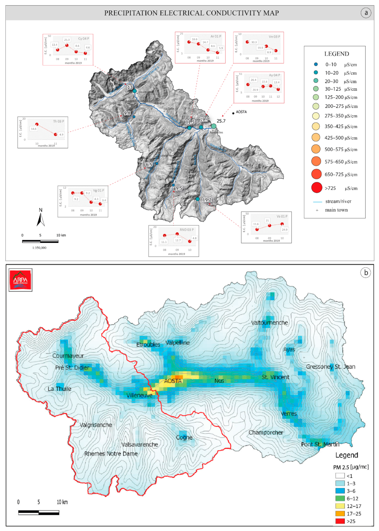
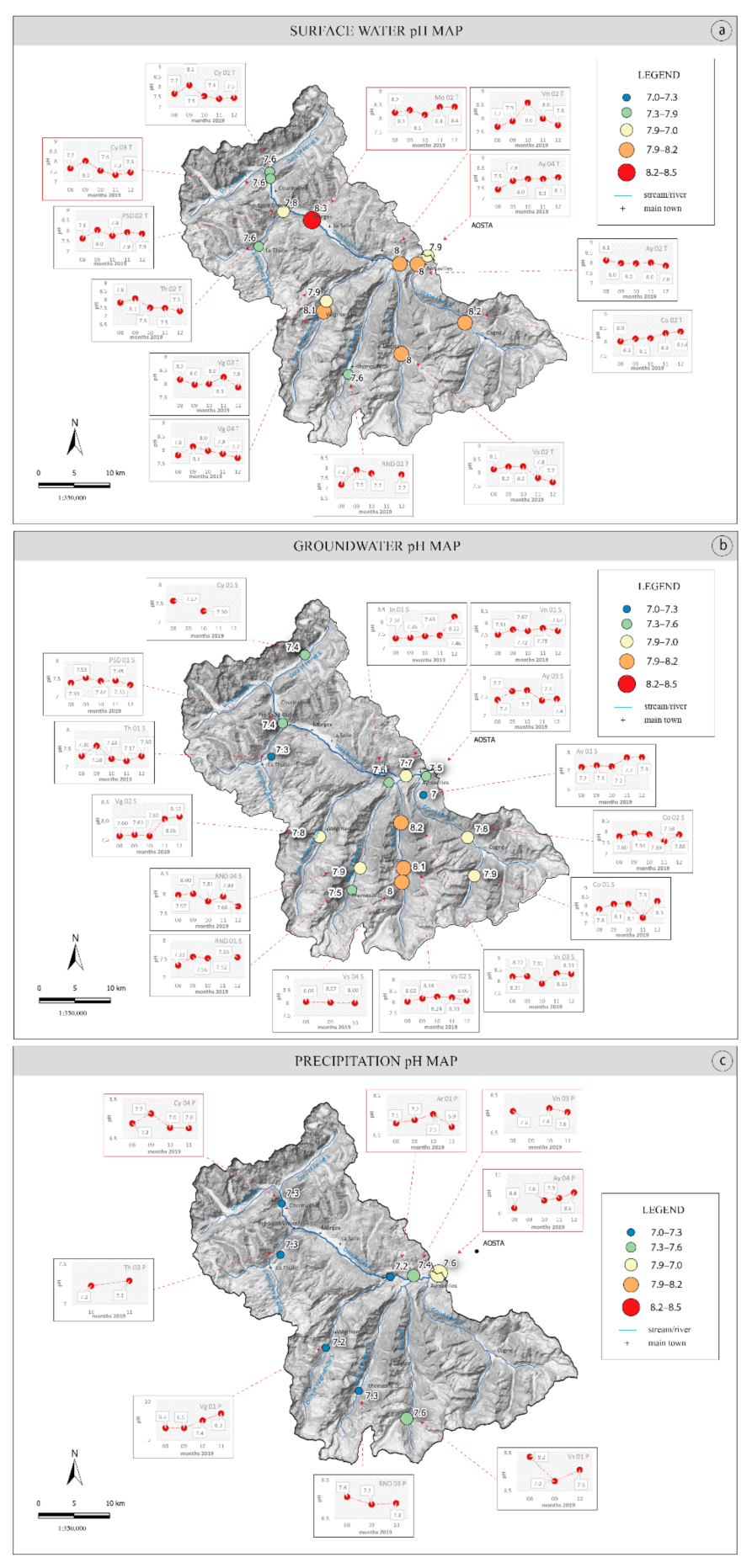
| Temperature (°C) | Electrical Conductivity (µS/cm) | pH | ||||||||||
|---|---|---|---|---|---|---|---|---|---|---|---|---|
| max | min | avg | std. dev. | max | min | avg | std. dev. | max | min | avg | std. dev. | |
| PRECIPITATION | - | - | - | - | 30.3 | 3.4 | 13.8 | 7.7 | 8.6 | 6.5 | 7.3 | 0.5 |
| SURFACE WATER | 12.9 | 0.1 | 6.8 | 3.5 | 519.0 | 46.4 | 182.1 | 104.1 | 8.6 | 7.2 | 7.9 | 0.3 |
| GROUNDWATER | 14.3 | 1.8 | 7.38 | 2.9 | 704.0 | 61.0 | 298.2 | 216.0 | 8.3 | 7.2 | 7.7 | 0.3 |
| HCO3− | F− | Cl− | ||||||||||
|---|---|---|---|---|---|---|---|---|---|---|---|---|
| min | max | avg | std. dev | min | max | avg | std. dev. | min | max | avg | std. dev. | |
| Rain | 2.6 | 16.1 | 7.4 | 4,1 | 0.02 | 0.03 | 0.2 | 0.00 | 0.06 | 1.04 | 0.24 | 0.24 |
| Surface water | 17.0 | 116.8 | 67.2 | 26.1 | 0 | 0.15 | 0.06 | 0.06 | 0.06 | 7.2 | 1.93 | 1.8 |
| Groundwater | 17.4 | 325 | 130.3 | 96.1 | 0 | 0.3 | 0.04 | 0.07 | 0 | 29.1 | 3.8 | 7.3 |
| NO3− | NO2− | SO4= | ||||||||||
| min | max | avg | std. dev. | min | max | avg | std. dev. | min | max | avg | std. dev. | |
| Rain | 0.14 | 2.4 | 1.02 | 0.70 | 0 | 0.46 | 0.10 | 0.13 | 0.23 | 1.18 | 0.64 | 0.3 |
| Surface water | 0 | 1.0 | 0.6 | 0.28 | 0 | 0.15 | 0.01 | 0.03 | 4.3 | 119.8 | 35.3 | 30.2 |
| Groundwater | 0.34 | 10.9 | 2.07 | 2.85 | 0 | 0.09 | 0.01 | 0.02 | 1.3 | 89.4 | 30.4 | 27.8 |
| Ca++ | K+ | Mg++ | ||||||||||
| min | max | avg | std. dev. | min | max | avg | std. dev. | min | max | avg | std. dev. | |
| Rain | 0.46 | 3.8 | 1.75 | 1.23 | 0.03 | 1.2 | 0.22 | 0.3 | 0 | 0.2 | 0.09 | 0.06 |
| Surface water | 9.2 | 64.9 | 29.6 | 14.0 | 0 | 1.9 | 1.04 | 0.48 | 0.6 | 7.9 | 3.56 | 2.14 |
| Groundwater | 9.0 | 77.5 | 36.04 | 20.9 | 0.4 | 5.4 | 1.6 | 1.1 | 0.5 | 39.0 | 9.75 | 11.3 |
| Na+ | NH4+ | |||||||||||
| min | max | avg | std. dev. | min | max | avg | std. dev. | |||||
| Rain | 0.1 | 1.2 | 0.27 | 0.28 | 0.08 | 3.0 | 0.62 | 0.74 | ||||
| Surface water | 0.25 | 6.86 | 2.13 | 1.6 | 0 | 0.6 | 0.15 | 0.14 | ||||
| Groundwater | 0.33 | 24.2 | 3.65 | 5.9 | 0 | 1.0 | 0.17 | 0.23 | ||||
| δ18O [‰] | δ2H [‰] | Deuterium Excess [‰] | ||||||||||
|---|---|---|---|---|---|---|---|---|---|---|---|---|
| max | min | avg | std.dev. | max | min | avg | std.dev. | max | min | avg | std.dev. | |
| PRECIPITATION (RAIN) | −2.5 | −15.3 | −7.7 | 4.4 | −10.5 | −106.7 | −49.3 | 32.2 | 22.3 | 1.7 | 12.7 | 5.0 |
| PRECIPITATION (SNOW) | −20.8 | −21.6 | −21.1 | 0.4 | −151.1 | −156.1 | −153.2 | 2.6 | 21.7 | 10.1 | 15.9 | 5.8 |
| SURFACE WATER | −10.8 | −14.4 | −13.1 | 0.8 | −71.6 | −101.9 | −91.1 | 6.8 | 19.3 | 8.8 | 13.9 | 3.0 |
| GROUNDWATER | −11.9 | −15.4 | −14.2 | 0.8 | −80.5 | −108.7 | −99.5 | 6.1 | 19.4 | 9.5 | 13.8 | 2.4 |
Publisher’s Note: MDPI stays neutral with regard to jurisdictional claims in published maps and institutional affiliations. |
© 2021 by the authors. Licensee MDPI, Basel, Switzerland. This article is an open access article distributed under the terms and conditions of the Creative Commons Attribution (CC BY) license (http://creativecommons.org/licenses/by/4.0/).
Share and Cite
Grappein, B.; Lasagna, M.; Capodaglio, P.; Caselle, C.; Luca, D.A.D. Hydrochemical and Isotopic Applications in the Western Aosta Valley (Italy) for Sustainable Groundwater Management. Sustainability 2021, 13, 487. https://0-doi-org.brum.beds.ac.uk/10.3390/su13020487
Grappein B, Lasagna M, Capodaglio P, Caselle C, Luca DAD. Hydrochemical and Isotopic Applications in the Western Aosta Valley (Italy) for Sustainable Groundwater Management. Sustainability. 2021; 13(2):487. https://0-doi-org.brum.beds.ac.uk/10.3390/su13020487
Chicago/Turabian StyleGrappein, Barbara, Manuela Lasagna, Pietro Capodaglio, Chiara Caselle, and Domenico Antonio De Luca. 2021. "Hydrochemical and Isotopic Applications in the Western Aosta Valley (Italy) for Sustainable Groundwater Management" Sustainability 13, no. 2: 487. https://0-doi-org.brum.beds.ac.uk/10.3390/su13020487