A Study of Inbound Logistics Mode Based on JIT Production in Cruise Ship Construction

Abstract

The cruise market has developed rapidly in recent years. The opulence of the cruise market has also augmented the demand for the cruise construction industry. Cruise ship construction is a huge and intricate heavy industry that can cause serious environmental problems. Therefore, optimal use of advanced logistics systems, to meet the demands at the lowest possible cost and unnecessary waste, has become a key issue. This paper developed two typical inbound logistics system modes based on JIT (Just In Time)-logistics policy and formulated two single-objective nonlinear models to simultaneously determine the ordering strategy under the inbound logistics system and the optimal selection strategy of two typical inbound logistics modes. Numerical experiments depicted the variations of optimal inbound logistics mode over three different kinds of cruise parts. These two models could provide insights in making inbound logistics decisions, and serve as a reference in the mass customization logistics service for cruise ship construction to control costs, which is helpful for promoting the sustainability of the cruise market.

1. Introduction

According to Cruise Lines International Association, the United States continues to account for the largest share of cruise demand (11.5%), followed by China (2.1%) in 2018. The Caribbean remains the key region of cruise line deployment (35.4%), followed by the Mediterranean (15.8%), Europe without the Mediterranean (11.3%), and China (6%). China is the main driver of passenger growth in Asia, accounting for almost half of regional passenger volume in 2015. China is quickly gaining ground in cruise development, given its growth rate of 183% in 2016 over 2015; it also ranks second in terms of total port calls and leads the Asian source market in terms of passenger volume. These findings demonstrate considerable demand for cruise experiences among Chinese travelers. Although the cruise industry in China remains in its infancy, this development is promising for various reasons, including the potential of the emerging middle class in China to support a robust cruise industry [1]. As a result, the number of orders for cruise ship construction has increased.

The cruise ship construction industry is one kind of heavy industry that can cause serious environmental problems. Green supply chain management had an emphasis on the characteristics of environment, flow, and coordination focuses [2]. Using lean manufacturing methods can reduce unnecessary steps, waste of human resources, and saving materials, which is helpful for pollution mitigation. Lean manufacturing is a strategy that aims to achieve a high level of performance using less effort, time, and material by eliminating waste and non-value-added activities from the entire cycle of operation. The principles of lean manufacturing encourage and improve teamwork, communication, efficient use of resources, and continuous improvement. As a system, it provides a better and more effective product, higher productivity, and greater customer loyalty [3].

At the Seatrade Asia Pacific cruise conference, Dr. Liu Zinan, President of China and North Asia region of Royal Caribbean International Cruise, shared how Royal Caribbean Cruises promote the sustainable development of the cruise industry. He proposed that the cruise industry is consumer-oriented. The sustainable development of the industry depends on the degree of satisfaction it creates for consumers, which, reducing cruise construction costs, can promote the sustainability of the market. Economical is one of the key characteristics for market sustainability [4].

The construction of cruise ships has three significant characteristics [5]. The first is high modularization. The second is that the parts span many fields. The third is that the number of parts is huge. Cruise ship construction is a complex project, involving a huge number of different kinds of parts. Many suppliers are involved in inbound logistics, and different parts have different logistics requirements, meaning that a link error can cause a chain reaction. Moreover, because cruise owners usually arrange the operating plan before the cruise ship is completed, construction delays can cause serious losses.

In summary, the implementation of the mass customization logistics service model has become an effective means for cruise ship construction to control costs in order to implement better sustainable operations strategies of the shipyard and promote the sustainability of the cruise market. However, although it is highly relevant to the actual needs, there has been little research on this topic. With this paper, we aimed to fill the gap in the research literature.

The remainder of the paper is organized as follows. Section 2 presents a literature review and outlines the innovative points and contributions of this paper. Section 3 describes the problem and puts forward the assumptions and notations for the model. Section 4 formulates the problem and establishes the modes of the two typical patterns of inbound logistics in cruise ship construction. Section 5 applies the models to numerical examples of shipyards. Section 6 discuss the managerial implications of numerical analysis. Section 7 concludes the paper and offers future research directions.

2. Literature Review

We focused our attention on the literature on inbound logistics modes in lean production and on models for selecting the optimal inbound logistics mode for different parts in cruise ship construction.

High-quality supply chain management is one of the key points in cruise ship construction, and inbound logistics is an essential key link in supply chain management. Previous research on inbound logistics has mostly been carried out on automobile manufacturing, steel plants, and fast-moving consumer goods industries, such as the dairy industry. Boysen et al. described the elementary process steps in part logistics in the automotive industry, from the initial call order to the return of empty part containers [6]. Thousands of parts and suppliers, a multitude of different types of equipment, and hundreds of logistics workers need to be coordinated so that the final assembly lines never run out of parts [6]. Mincuzzi et al. investigated the potential of a data integration solution to support a set of interacting decision-support tools for inbound logistics in automotive manufacturing [7]. Mukherjee et al. presented an approach for inbound logistics capacity design by uncovering the hidden capacities of an integrated steel plant’s raw material handling system [8]. Costa et al. identified how the relationships between inbound logistics (IL) activities can contribute to organizational resilience. In total, two in-depth case-based studies were conducted in the dairy industry [9]. Fink and Benz presented a process-oriented approach for the measurement and planning of IL flexibility in global production networks [10].

Compared with automobile factories and the fast-moving consumer goods industry, parts in cruise construction are much more complex. Most of the parts in automobile factories are standard parts that can easily be transported to the assembly line. The products of automobile factories have a high degree of similarity and can be built on a large scale. However, shipyards are different: because each cruise ship is designed individually, the proportion of standard parts is much lower than in an automobile factory. Semini et al. concluded that the ship design and construction industry serves a considerable range of market segments, with different levels of required customization, different demand volumes, and other product and market variations [11], especially in cruise ship construction. It is, therefore, worthwhile to conduct research on IL in line with the characteristics of cruise ship construction to fill the gaps in the research literature. Kovacs and Kot introduced Industry 4.0 conception which will change the production and logistical processes drastically [12]. Prajogo indicated that lean production processes have a positive effect on inbound supply performance [13].

Warnecke described “lean production” as an intellectual approach consisting of a system of measures and methods which, when taken together, have the potential to produce a lean and, therefore, a particularly competitive state in a company [14]. Shah and Ward addressed the confusion and inconsistency associated with “lean production,” and their configuration theory provides the theoretical underpinnings to explain the synergistic relationships among its underlying components [15]. Storch and Lim explored lean production in the shipbuilding industry. They claimed that the basis for the establishment of lean thinking in shipbuilding is the appropriate application of group technologies through the use of a product-oriented work-breakdown structure [16]. The IL mode is one of the group of technologies involved in lean production in shipbuilding. Supply chain management (SCM) in shipbuilding depends essentially on improving the relationship with suppliers and adopting appropriate information and communication technology (ICT) [17]. Saudi et al. indicates that lean practices have significant positive relationship with supply chain performance [18]. Fullerton et al. conducted a study that demonstrates that implementing the continuous quality improvement and waste-reduction practices embodied in the JIT philosophy can enhance firm competitiveness. Their study indicates that JIT is a vital manufacturing strategy for building and sustaining a competitive advantage [19]. JIT purchasing has a direct positive relationship with agile manufacturing, and the positive relationship between JIT production and agile manufacturing is mediated by JIT purchasing [20]. Belekoukias et al. indicated that JIT and automation have the strongest significance for operational performance, whereas kaizen, TPM (Total Productive Maintenance), and VSM (Value Stream Mapping) seem to have lesser, or even negative, effects on it [21]. Therefore, an IL mode based on a JIT production strategy will facilitate the smooth implementation of production plans in an efficient and economical way. Recently, many scholars have studied IL planning in JIT policy. Schoeneberg et al. presented a two-stage stochastic mixed integer linear programming model to determine robust delivery profile assignments under uncertain and infrequent demands and complex tariff systems [22]. Lee et al. proposed a simultaneous control method for combining vehicle scheduling and inventory control for IL for an Original Equipment Manufacturing (OEM) manufacturer to achieve a short production time and implement JIT policy [23]. Straka et al. focused on the job sequence problem of transport processes at the rail terminal and used computer simulation system for the solution [24]. Calabro et al. presented the first results of an agent-based model aimed at solving a Capacitated Vehicle Routing Problem (CVRP) for IL using a novel Ant Colony Optimization (ACO) algorithm, developed and implemented in the Net Logo multi-agent modeling environment [25].

In summary, most previous studies have focused on the micro level of path and inventory research, and the fields of application are mostly in areas with a high degree of standardization. The design factors of parts logistics systems encompass logistics network design, parts vendor selection, and transportation mode selection [26]. The lack of research on macro fields thus makes it necessary to conduct research on IL modes based on JIT production in cruise ship construction.

3. Problem Description, Assumption, and Notation

3.1. Problem Description

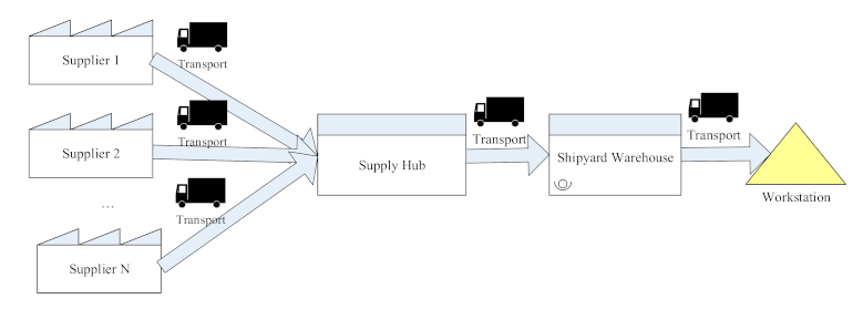
Suppose there is a shipyard that adopts a JIT-logistics (small lot size delivery) policy for cruise ship construction; there will be two feasible IL modes for collecting parts [27,28]. Mode 1 consists of multiple suppliers, a supply hub, a shipyard warehouse, and a workstation. Suppliers transport parts to the supply hub at certain intervals called $R_{sh}$. The parts are then centralized and stored in the supply hub, and then transported to the shipyard warehouse at certain intervals called $R_{hw}$. Finally, the parts are distributed from the shipyard warehouse to the workstation. The processes in Mode 1 are described in Figure 1.

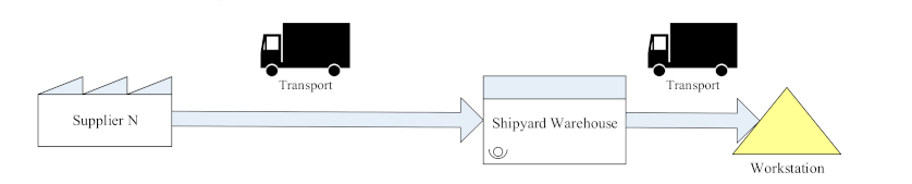
Mode 2 consists of one supplier, a shipyard warehouse, and a workstation. Parts are transported directly by the supplier to the shipyard warehouse at certain intervals called $R_{sw}$ and then distributed to the workstation. The processes in Mode 2 are described in Figure 2.

Based on the background of cruise ship construction, the main questions of this study are:

Q1: How should the logistics costs in large cruise ship construction be quantified?

Q2: How should the optimal logistics mode be decided on, depending on the kinds of parts?

Q3: How does demand for certain parts impact the operational decisions of the logistics model?

Q4: What managerial implications can be derived from this study for shipyards to implement better sustainable operations strategies?

To answer these questions, we developed two typical inbound logistics system modes based on JIT-logistics policy [29,30], to simultaneously determine the ordering strategy under the inbound logistics system and the optimal selection strategy of two typical inbound logistics modes. The objective of Model 1 and Model 2 is to minimize the total inbound logistics cost of parts in cruise construction [31,32].

3.2. Assumption and Notation

Assumption 1:

The supplier has enough capacity to ensure the supply of the shipyard. The shipyard warehouse has enough space to meet the requirements.

Assumption 2:

The supplier products parts at certain intervals. The production volume equals the demand for shipyard workstations in the interval.

Assumption 3:

The supplier transport parts at the same intervals. The transportation volume equals the demand for shipyard workstations in the interval. The Transport Lead Time remains unchanged, assuming that the value is 0. The production intervals are equal to the transportation intervals of the supplier.

Assumption 4:

In supply hub mode, the supply hub is near the shipyard. High-frequency transportation is conducted to reduce the storage in the shipyard warehouse, so the transportation interval from the supply hub to the shipyard warehouse is relatively short. Suppose the transportation interval from the supplier to the supply hub is N times that from the supply hub to the shipyard warehouse. In the optimum design, N is an integer.

Assumption 5:

Under normal conditions, the transportation time from the supply hub to the shipyard warehouse, from the shipyard warehouse to the workstation, and from the supplier to the shipyard warehouse or supply hub remain unchanged and determined [33].

Assumption 6:

Delays may occur during transportation or cargo may be damaged. For the sake of catching up with the schedule, shipyard workers may have to work overtime. Overtime is related to delays.

Assumption 7:

The supply hub has safety stock to mitigate the effect of delays.

Assumption 8:

Parts will incur a certain cost when stored in the supply hub and shipyard warehouse. As a storage area, the storage cost of the supply hub is lower than that of the shipyard warehouse.

Assumption 9:

The transportation cost each time from the supply hub to the shipyard warehouse remains unchanged.

Assumption 10:

The transportation cost from the shipyard warehouse to the workstation is 0.

Table 1. Model notation and description.

Notation	Description
$i$	The code for the parts
$d_i$	The demand of the shipyard workstation for parts i per unit time.
$S_i$	Setup production cost of parts i per unit batch
$O_i$	Variable production cost of parts i per unit batch
$E_i$	Extra production cost of parts i
$P_i$	Production time of parts i
$D_{is}$	The distance between supplier and shipyard
$h_{si}$	Storage cost of parts i in the supplier
$h_{hi}$	Storage cost of parts i in the supply hub
$h_{wi}$	Storage cost of parts i in the shipyard warehouse
$h_f$	Storage cost of Safety stock in supply hub
$b$	Operating cost of supply hub
$T_{fsh}$	Fixed transportation cost of parts i from the supplier to the supply hub per unit batch
$T_{vsh}$	Variable transportation cost of parts i from the supplier to the supply hub per unit batch
$T_{fsw}$	Fixed transportation cost of parts i from the supplier to the shipyard warehouse per unit batch
$T_{vsw}$	Variable transportation cost of parts i from the supplier to the shipyard warehouse per unit batch
$T_{hw}$	Transportation cost of parts i from the supply hub to the shipyard warehouse per unit batch
$C_{sh}$	Transport capacity from the supplier to the supply hub
$C_{sw}$	Transportation capacity from the supplier to the shipyard warehouse
$C_{hw}$	Transportation capacity of parts i from the supply hub to the shipyard warehouse
$G_{di}$	Cargo damage rate of parts i
$Y_l$	Labor pay of shipyard per unit time
$Y_o$	Overtime pay of shipyard per unit time
$R_{sh}$	Replenishment interval of parts i from the supplier to the supply hub per unit time.
$R_{sw}$	Replenishment interval of parts i from the supply hub to the shipyard warehouse per unit time.
$R_{hw}$	Replenishment interval of parts i from the supply hub to the shipyard warehouse per unit time.
$L$	The delay of parts i in transportation
$T{C}_i$	Total inbound logistics cost of parts i.

shows notations and descriptions in the model.

4. Model Specification

4.1. Mode 1: Supply Hub

4.1.1. Model Objective Function

Objective: To minimize the total IL cost of part I [34,35].

$C_1$ represents the production cost per unit time of parts i, which is composed of fixed cost and variable cost. Variable cost $O_i$ is determined by the quantity of production $R_{sh}{d}_i$. $O_0$ is a parameter[36,37].

$$C_1=\frac{S_i+O_i}{R_{sh}}$$

(1)

$$O_i=O_0\times R_{sh}{d}_i$$

(2)

$C_2$ represents the transportation cost per unit time of parts i. In (3), the first term represents the transportation cost from the supplier to the supply hub per unit time, which is composed of fixed costs and variable costs. The second term represents the transportation cost per unit time when parts i are transported from the supply hub to the shipyard warehouse. Variable cost $T_{vsh}$ is determined by the distance between the supplier and the supply hub $D_{is}$. $T_0$ is a parameter.

$$C_2=\frac{T_{fsh}+T_{vsh}}{R_{sh}}\times \lceil \frac{d_i{R}_{sh}}{C_{sh}}\rceil +\frac{T_{hw}}{R_{hw}}\times \lceil \frac{R_{hw}}{C_{hw}}\rceil$$

(3)

$$T_{vsh}=T_0\times D_{is}$$

(4)

$C_3$ represents the storage cost of parts i. In (5), the first term represents the storage cost of parts i in the supplier warehouse per unit time. The second term represents the storage cost of parts i in the supply hub per unit time. The third term represents the storage cost of parts i in the shipyard warehouse per unit time [38].

$$C_3=\frac{1}{2}{h}_{si}{p}_i{d}_i^2{R}_{sh}+\frac{1}{2}{h}_{hi}{d}_i\left(R_{sh}-R_{hw}\right)+\frac{1}{2}{h}_{wi}{d}_i{R}_{hw}$$

(5)

$C_4$ represents the cargo damage cost of parts i. Cargo damage also causes delays. However, there is safety stock to avoid this.

$$C_4=E_i\times G_{di}\times d_i$$

(6)

$C_5$ represents the maintenance cost of safety stock and operating cost of the supply hub.

$$C_5=h_f+b$$

(7)

4.1.2. Model Constraints

The constraints of the model are based on the actual situation; the replenishment interval must be greater than 0. So, $R_{sh}>0c>0$.

Formula $R_{hw}\le C_{hw}$ is the constraint of the logistics distribution capacity of the supply hub. $d_i{R}_{sh}\le C_{sh}$ is the constraint of the logistics distribution capacity of the supplier.

Because of the limited area of the workstation, the distribution interval from the shipyard warehouse to the workstation is generally short. In most cases, a single delivery equals 6- or 12-hours’ consumption on the workstation, whereas the distribution interval of a supplier to the shipyard warehouse or supply hub is relatively long. In optimum operation, the distribution interval is an integral multiple of that from the shipyard warehouse to the workstation. Therefore, $R_{sh}=N{R}_{hw}N\ge 1,\mathrm{where}N\mathrm{is}\mathrm{an}\mathrm{integral}$ [39].

4.1.3. Joint Decision Model and Solution

$$minT{C}_i={\displaystyle \sum }_{i=1}^5{C}_i=\frac{S_i+O_0\times R_{sh}{d}_i}{R_{sh}}+\frac{T_{fsh}+T_{vsh}}{R_{sh}}\times \lceil \frac{d_i{R}_{sh}}{C_{sh}}\rceil +\frac{T_{hw}}{R_{hw}}\times \lceil \frac{d_i{R}_{hw}}{C_{hw}}\rceil +\frac{1}{2}{h}_{si}{p}_i{d}_i^2{R}_{sh}+\frac{1}{2}{h}_{hi}{d}_i\left(R_{sh}-R_{hw}\right)+\frac{1}{2}{h}_{wi}{d}_i{R}_{hw}+E_i\times G_{di}\times d_i+h_f+b$$

(8)

$S.T.$

$$R_{sh}>0 R_{hw}>0$$

(9)

$$d_i{R}_{hw}\le C_{hw}$$

(10)

$$d_i{R}_{sh}\le C_{sh}$$

(11)

$$R_{sh}=N{R}_{hw}N\ge 1,\mathrm{N}\mathrm{is}\mathrm{an}\mathrm{integral}$$

(12)

Plug (9) to Formula (12) into objective function (8):

$$minT{C}_i=\frac{S_i}{N{R}_{hw}}+O_i\times d_i+\frac{T_{fsh}+T_{vsh}}{N{R}_{hw}}+\frac{T_{hw}}{R_{hw}}+\frac{1}{2}N{h}_{si}{p}_i{d}_i^2{R}_{hw}+\frac{1}{2}{d}_i{R}_{hw}{d}_i\times \left[\left(N-1\right)h_{hi}+h_{wi}\right]+E_i\times G_{di}\times d_i+h_f+b$$

(13)

Derivation of (13):

$$\mathrm{Because}\frac{d^{2}T{C}_i}{d{R}_{hw}^2}=2\times \frac{S_i+N{T}_{hw}+T_{fsh}+T_{vsh}}{N{R}_{hw}^3}>0$$

(14)

$T{C}_i\left(R_{hw}\right)$ is a lower convex function.

$T{C}_i\left(R_{hw}\right)$ has a minimum value and when:

$$\frac{dT{C}_i}{d{R}_{hw}}=-\frac{S_i+N{T}_{hw}+T_{fsh}+T_{vsh}}{N{R}_{hw}^2}+\frac{1}{2}N{h}_{si}{p}_i{d}_i^2+\frac{1}{2}{d}_i\left[h_{hi}\left(N-1\right)+h_{wi}\right]=0$$

(15)

$$R_{ws}=\sqrt{\frac{2\times \left(S_i+N{T}_{hw}{T}_{fsh}+T_{vsh}\right)}{N^2{h}_{si}{p}_i{d}_i^2+N{d}_i\left[h_{hi}\left(N-1\right)+h_{wi}\right]}}$$

(16)

$T{C}_i\left(R_{hw}\right)$ obtains a minimal value [40].

4.2. Mode 2: Direct Sending

4.2.1. Model Objective Function

Objective: To minimize the total IL cost of part i.

$C_1$ represents the production cost per unit time of parts i, which is composed of fixed cost and variable cost. Variable cost $O_i$ is determined by the quantity of production $R_{sw}{d}_i$. $O_0$ is a parameter [36,37].

$$C_1=\frac{S_i+O_i}{R_{sw}}$$

(17)

$$O_i=O_0\times R_{sw}{d}_i$$

(18)

$C_2$ represents the transportation cost per unit time of parts i. Formula (16) represents the transportation cost from the supplier to the shipyard warehouse per unit time, which is composed of fixed costs and variable costs. Variable cost $T_{vsw}$ is determined by the distance between the supplier and the shipyard warehouse $D_{is}$. $T_0$ is a parameter.

$$C_2=\frac{T_{fsw}+T_{vsw}}{R_{sw}}\times \lceil \frac{d_i{R}_{sw}}{C_{sw}}\rceil$$

(19)

$$T_{vsw}=T_0\times D_{is}$$

(20)

$C_3$ represents the storage cost of parts i. In (5), the first term represents the storage cost of parts i in the supplier warehouse per unit time. The second term represents the storage cost of parts i in the shipyard warehouse per unit time.

$$C_3=\frac{1}{2}{h}_{si}{p}_i{d}_i^2{R}_{sw}+\frac{1}{2}{h}_{wi}{d}_i{R}_{sw}$$

(21)

$C_4$ represents the cargo damage cost of parts i. The first term represents the extra production cost of parts i per unit time.

$$C_4=E_i\times G_{di}\times d_i$$

(22)

$C_5$ represents the delay cost of parts i in transportation. The delay $L$ is due to cargo damage and transportation. The first term represents the delay cost due to cargo damage if assembling parts i is a key step. The formula $L\times Y_i$ indicates the waste of labor because assembling parts i is a key step and shipyard workers have to wait for the parts i. The formula $kL\times Y_o$ indicates the overtime cost. For the sake of catching up with the schedule, shipyard workers have to work overtime. Overtime is related to delays. k is a parameter. The second term represents the delay cost if assembling parts i is not a key step. If assembling parts i is a key step in the construction, $M_1=1,M_2=0$, else $M_1=0,M_2=1$.

$$C_5=\left(L\times Y_i+kL\times Y_o\right)M_1+\left(kL\times Y_o\right)M_2$$

(23)

4.2.2. Model Constraints

Among the constraints of the model, the formula$R_{wt}>0$ indicates that the replenishment interval must be greater than 0;

Formula $d_i{R}_{sw}\le C_{sw}$ is the constraint of the logistics distribution capacity of the supplier.

4.2.3. Joint Decision Model and Solution

$$minT{C}_i={\displaystyle \sum }_{i=1}^5{C}_i=\frac{S_i+O_0\times R_{sw}{d}_i}{R_{sw}}+\frac{T_{fsw}+T_{vsw}}{R_{sw}}\times \lceil \frac{d_i{R}_{sw}}{C_{sw}}\rceil +\frac{1}{2}{h}_{si}{p}_i{d}_i^2{R}_{sw}+\frac{1}{2}{h}_{wi}{d}_i{R}_{sw}+E_i\times G_{di}+\left(k\left(p_i+m{D}_{is}\right)\times Y_o\right)M_2+\left(L\times Y_i+kL\times Y_o\right)M_1+\left(kL\times Y_o\right)M_2$$

(24)

$S.T.$

$$R_{sw}>0$$

(25)

$$d_i{R}_{sw}\le C_{sw}$$

(26)

Plug Formulas (25)–(26) into objective function (24):

$$minT{C}_i=\frac{S_i}{R_{sw}}+O_o\times d_i+\frac{T_{fsw}+T_{vsw}}{R_{sw}}+\frac{1}{2}{h}_{si}{p}_i{d}_i^2{R}_{sw}+\frac{1}{2}{h}_{wi}{d}_i{R}_{SW}+E_i\times G_{di}+\left(k\left(p_i+m{D}_{is}\right)\times Y_o\right)M_2+\left(L\times Y_i+kL\times Y_o\right)M_1+\left(kL\times Y_o\right)M_2$$

(27)

Derivation of (27)

Because:

$$\mathrm{Because}\frac{d^{2}T{C}_i}{d{R}_{sw}^2}=2\times \frac{S_i+T_{fsw}+T_{vsw}}{R_{sw}^3}>0$$

(28)

$T{C}_i\left(R_{sw}\right)$ is a lower convex function.

$T{C}_i\left(R_{sw}\right)$ has a minimum value and when:

$$\frac{dT{C}_i}{d{R}_{sw}}=-\frac{S_i+T_{fsw}+T_{vsw}}{R_{sw}^2}+\frac{1}{2}{h}_{si}{p}_i{d}_i^2+\frac{1}{2}{h}_{wi}{d}_i=0$$

(29)

$$R_{sw}=\sqrt{\frac{2S_i+T_{fsw}+T_{vsw}}{h_{si}{p}_i{d}_i^2+h_{wi}{d}_i}}$$

(30)

$T{C}_i$ obtains an optimal value [40].

5. Analysis of Numerical Examples and Model Application

5.1. Parameters Settings

As an illustration, three typical parts in two IL mode are discussed. The numerical value of each parameter is provided by China State Shipbuilding Corporation Limited. The input parameters for the base example are given in the

Table A1. Parameters settings of ship plates in Mode 1.

Parameters	Units	Value
$d_i$	quantity	125
$S_i$	thousand RMB/batch	10
$O_i$	thousand RMB/quantity	3
$E_i$	thousand RMB/quantity	3.1
$P_i$	month	0.05
$D_{is}$	km	200
$h_{si}$	thousand RMB/month*quantity	1
$h_{hi}$	thousand RMB/month*quantity	0.5
$h_{wi}$	thousand RMB/month*quantity	1
$h_f$	thousand RMB/month	30
$b$	thousand RMB/month	15
$N$	/	5
$T_{fsh}$	thousand RMB/batch	5
$T_0$	thousand RMB/km	0.1
$T_{hw}$	thousand RMB/batch	0.2
$C_{sh}$	quantity	10,000
$C_{hw}$	quantity	1000
$G_{di}$	/	0.03

,

Table A2. Parameters settings of ship plates in Mode 2.

Parameters	Units	Value
$d_i$	quantity	125
$S_i$	thousand RMB/batch	10
$O_i$	thousand RMB/quantity	3
$E_i$	thousand RMB/quantity	3.1
$P_i$	month	0.05
$D_{is}$	km	200
$h_{si}$	thousand RMB/month*quantity	1
$h_{hi}$	thousand RMB/month*quantity	0.5
$h_{wi}$	thousand RMB/month*quantity	1
$T_{fsw}$	thousand RMB/batch	5
$C_{sw}$	quantity	1000
$G_{di}$	/	0.01
$Y_l$	thousand RMB/month	100
$Y_o$	thousand RMB/month	110
$L$	month	0.2
$k$	/	0.4
$M_1$	/	0
$M_2$	/	1

,

Table A3. Parameters settings of prefabricated cabins in Mode 1.

Parameters	Units	Value
$d_i$	quantity	30
$S_i$	thousand RMB/batch	25
$O_i$	thousand RMB/quantity	40
$E_i$	thousand RMB/quantity	50
$P_i$	month	0.2
$D_{is}$	km	1500
$h_{si}$	thousand RMB/month*quantity	3
$h_{hi}$	thousand RMB/month*quantity	1.5
$h_{wi}$	thousand RMB/month*quantity	3
$h_f$	thousand RMB/month	80
$b$	thousand RMB/month	20
$N$	/	5
$T_{fsh}$	thousand RMB/batch	50
$T_0$	thousand RMB/km	0.1
$T_{hw}$	thousand RMB/batch	1
$C_{sh}$	quantity	10,000
$C_{hw}$	quantity	1000
$G_{di}$	/	0.05

,

Table A4. Parameters settings of prefabricated cabins in Mode 2.

Parameters	Units	Value
$d_i$	quantity	30
$S_i$	thousand RMB/batch	25
$O_i$	thousand RMB/quantity	40
$E_i$	thousand RMB/quantity	50
$P_i$	month	0.2
$D_{is}$	km	1500
$h_{si}$	thousand RMB/month*quantity	3
$h_{hi}$	thousand RMB/month*quantity	1.5
$h_{wi}$	thousand RMB/month*quantity	3
$T_{fsw}$	thousand RMB/batch	50
$C_{sw}$	quantity	1000
$G_{di}$	/	0.001
$Y_l$	thousand RMB/month	80
$Y_o$	thousand RMB/month	88
$L$	month	0.1
$k$	/	0.4
$M_1$	/	1
$M_2$	/	0

,

Table A5. Parameters settings of outfitting item in Mode 1.

Parameters	Units	Value
$d_i$	quantity	500
$S_i$	thousand RMB/batch	2
$O_i$	thousand RMB/quantity	0.3
$E_i$	thousand RMB/quantity	0.3
$P_i$	month	0.08
$D_{is}$	km	180
$h_{si}$	thousand RMB/month*quantity	0.5
$h_{hi}$	thousand RMB/month*quantity	0.25
$h_{wi}$	thousand RMB/month*quantity	0.5
$h_f$	thousand RMB/month	5
$b$	thousand RMB/month	5
$N$	/	5
$T_{fsh}$	thousand RMB/batch	1.5
$T_0$	thousand RMB/km	0.1
$T_{hw}$	thousand RMB/batch	0.2
$C_{sh}$	quantity	100,000
$C_{hw}$	quantity	10,000
$G_{di}$	/	0.02

and

Table A6. Parameters settings of outfitting item in Mode 2.

Parameters	Units	Value
$d_i$	quantity	500
$S_i$	thousand RMB/batch	2
$O_i$	thousand RMB/quantity	0.3
$E_i$	thousand RMB/quantity	0.3
$P_i$	month	0.08
$D_{is}$	km	180
$h_{si}$	thousand RMB/month*quantity	0.5
$h_{hi}$	thousand RMB/month*quantity	0.25
$h_{wi}$	thousand RMB/month*quantity	0.5
$T_{fsw}$	thousand RMB/batch	0.8
$C_{sw}$	quantity	10,000
$G_{di}$	/	0.01
$Y_l$	thousand RMB/month	120
$Y_o$	thousand RMB/month	132
$L$	month	0.08
$k$	/	0.4
$M_1$	/	0
$M_2$	/	1

.

5.2. Analysis of the Effect of Ordering Strategy on the Total Logistics Cost

To test the effect of ordering strategy on the total logistics cost. The values of other parameters are shown in Table A1. We use Formulas (16) and (30) to calculate the optimal ordering strategy in two IL mode, respectively. The optimal $R_{sh}=0.29$, $R_{sw}=0.28$. $R_{sh}$ is changed from 0.09 to 0.49 in sequence. $R_{sw}$ is changed from 0.08 to 0.48 in sequence. The results are shown in

Table 2. The effect of ordering strategy on the total logistics cost.

$Supply Hub R_{sh}$	Supply Hub $\mathit{T}{\mathit{C}}_{\mathit{i}}$	Direct Sending ${\mathit{R}}_{\mathit{s}\mathit{w}}$	Direct Sending $\mathit{T}{\mathit{C}}_{\mathit{i}}$
0.09	1328.8	0.08	1614.1
0.14	863.7	0.13	907.6
0.19	745.9	0.18	762.0
0.24	701.2	0.23	709.8
0.29	679.9	0.28	690.2
0.34	683.2	0.33	685.7
0.39	691.1	0.38	689.4
0.44	702.0	0.43	698.1
0.49	715.0	0.48	710.1

.

Observation 1: In Mode 1, when the value of $R_{sh}$ increases from 0.09 to 0.49, the value of TC (total cost) decreases first and then increases, and when $R_{sh}$ reaches the optimal value, the TC value reaches the minimum. Similar conclusions are obtained for Mode 2.

5.3. Analysis of the Effect of N on the Total Logistics Cost of Mode1

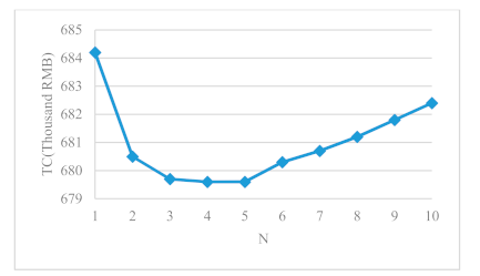
To test the effect of different N values on the total logistics cost and select the optimal value of N in Mode 1, N is changed from 1 to 10 in sequence. The demand for ship plate per unit time was set, $d_1=125$. The values of other parameters are shown in Table A1. The results are shown in Figure 3. The corresponding optimal replenishment interval $R_{sh}$ and $R_{hw}$ of different N values are calculated and shown in

Table 3. The effect of different n values on optimal replenishment interval.

$N$	Optimal ${\mathit{R}}_{\mathit{s}\mathit{h}}$	Optimal ${\mathit{R}}_{\mathit{h}\mathit{w}}$
1	0.278	0.278
2	0.284	0.142
3	0.287	0.096
4	0.289	0.072
5	0.290	0.058
6	0.291	0.049
7	0.292	0.042
8	0.293	0.037
9	0.294	0.033
10	0.295	0.030

.

Observation 2: For ship plate, when the value of N increases from 1 to 10, the optimal $R_{sh}$ increases and the optimal $R_{hw}$ decreases, the value of TC decreases first and then increases, and when N equals 4 and 5, the TC value reaches the minimum.

5.4. Analysis of the Effect of Demand on the Decision the IL Mode Decision

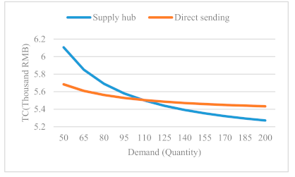
To test the effect of demand for parts on the IL mode decision, we changed it from 50 to 200 and observed its effect on the total logistics cost and the unit logistics cost of different logistics modes. The numerical values of other parameters were settled according to Table 2 and Table 3. Supply hub $T{C}_i$, Direct sending $T{C}_i$represent, respectively, the total IL costs of Mode 1 and Mode 2.

Table 4. Total costs and average cost comparison of ship plate in Mode 1 and Mode 2.

${\mathit{d}}_{\mathit{i}}$	Supply Hub $\mathit{T}{\mathit{C}}_{\mathit{i}}$	Direct Sending $\mathit{T}{\mathit{C}}_{\mathit{i}}$	Supply Hub $\frac{\mathit{T}{\mathit{C}}_{\mathit{i}}}{{\mathit{d}}_{\mathit{i}}}$	Direct Sending $\frac{\mathit{T}{\mathit{C}}_{\mathit{i}}}{{\mathit{d}}_{\mathit{i}}}$
50	305.3	284.2	6.11	5.68
65	380.3	364.6	5.85	5.61
80	455.2	445.0	5.69	5.56
95	530.1	525.2	5.58	5.53
110	605.0	605.5	5.50	5.50
125	679.8	685.7	5.44	5.49
140	754.8	765.9	5.39	5.47
155	829.7	846.1	5.35	5.46
170	904.5	926.2	5.32	5.45
185	979.4	1006.5	5.29	5.44
200	1054.3	1086.6	5.27	5.43

shows the changing trend for the total IL costs of the different modes with increasing demand for ship plate when the transportation path is determined.

Observation 3: The results illustrate that with the increase in demand for ship plate, the unit logistics costs of Mode 1 and Mode 2 are decreasing. When the demand for ship plate is small, Mode 2 costs less. However, with the increase in demand for ship plate, the optimal inbound logistics mode changes; the trend is shown in Figure 4.

5.5. Model Application

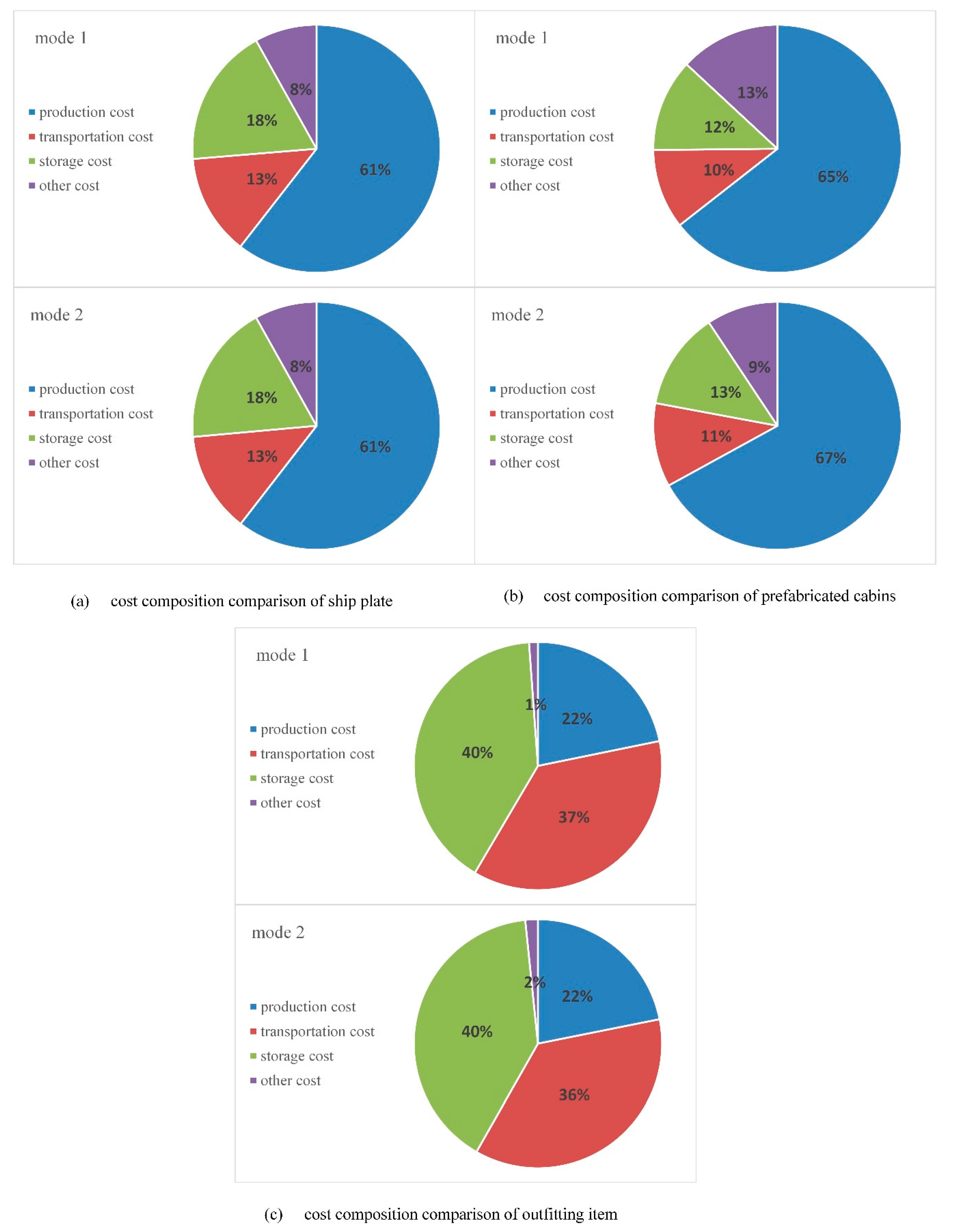
We set the demand for ship plate per unit time as $d_1=125$. , the demand for prefabricated cabins per unit time as $d_2=30$. , and the demand for outfitting item per unit time as $d_3=500$. The values of other parameters are shown in Table A1, Table A2, Table A3, Table A4, Table A5 and Table A6. We use Formulas (16) and (30) to determine the optimal ordering strategy in two IL mode, respectively.

Table 5. Total costs comparison of three typical parts in Mode 1 and Mode 2.

Parts	Supply Hub $\mathit{T}{\mathit{C}}_{\mathit{i}}$	Direct Sending $\mathit{T}{\mathit{C}}_{\mathit{i}}$	Optimal IL Mode
ship plate	679.8	685.7	Supply hub
prefabricated cabins	1912.4	1831.1	Direct sending
outfitting item	827.7	827.3	Direct sending

shows the total inbound logistic costs of different modes with different kinds of parts when the demand for each part is determined. Less cost mode is selected as the optimal IL mode. Figure 5 shows the proportion of the total cost, with production cost, transportation cost, storage cost, and others.

6. Discussion

The model developed in this study determines the optimal ordering strategy and IL mode choices. To numerically determine the impact of parts on ordering strategy and optimal IL mode choices, three different parts were opted for analysis in this study. The numerical simulations conducted imparts the following insights:

The optimal ordering strategy revealed through the developed model significantly optimize the IL cost savings. The optimal values of $R_{sh}$/$R_{sw}$ imparts the minimum IL costs. While the assumption 3 is deduced as an ideal pre-condition, the production intervals of the supplier at site may differ from the optimal transportation intervals of $R_{sh}$/$R_{sw}$. In this case, the achievement of optimal $R_{sh}$/$R_{sw}$ is impractical, assigning it a closest value may impart relatively optimal ordering strategy.

Moreover, the optimal IL model vary as a function of demand for the same parts under consideration. Similarly, to reduce the overall logistics cost for changing production plan or construction phase in cruise construction, the decision-making process for the management can be augmented by selecting the optimal logistics mode. This aspect optimizes various phases in cruise ship construction where the demand for parts is constantly changing. This dynamic decision-making aspect of the developed model augmenting the IL management enhance the novelty of this study in comparison to the available concurrent literature.

The optimal IL mode and the overall cost reduction varies for each part. For example, the prefabricated cabins have a remarkable overall logistics cost reduction. Hence, the developed model quantifies the IL costs and decision makers are enabled to select the optimal mode for each part and therefore reduce the overall logistics cost of the cruise ship construction.

The variation in cost for same parts in different IL modes is insignificant. However, for different parts in the same mode, this variation is remarkable. This change in costs is attributed to the salient characteristics of each part.

7. Conclusions

This paper analyzed two different modes of IL in cruise ship construction and established two IL cost models. Given the above analysis, we believe that it has a certain theoretical and practical significance.

In terms of theoretical significance, this paper developed IL cost optimization models based on JIT-logistics policy and sustainable logistics management in cruise ship construction. The model quantified the inbound logistics, which is a key issue in the cruise ship construction. In total, two decision models were formulated, and numerical examples were applied to demonstrate the application of the models.

In terms of practical significance, this paper discussed some of the key issues in the mass customization of logistics services. From the results of the numerical examples and the findings of the experiments, we answered the proposed questions and obtained conclusions as follows:

For cost composition (production costs, transportation costs, storage costs) of different kinds of parts in IL of cruise ship construction, there is a relationship. For example, the relationships in the costs involved in ship plate are: production cost > storage cost > transportation cost.

For the same parts in cruise ship construction, the decision-maker can choose the optimal IL mode according to the demand.

For different kinds of parts in cruise ship construction, the optimal logistics mode is also different. The model in this paper can serve as a reference for logistics decisions.

For the inbound logistics adopting JIT policy in cruise ship construction, the optimal replenishment interval should be selected to minimize the total costs.

The numerical examples above generate management implications for logistics management. The model in this paper can serve as a reference for logistics decisions and provide a direction for improving the efficiency and controlling the logistics costs in cruise ship construction.

This paper has some limitations, and some possible extensions can be made in the future. For example, it assumes that the replenishment interval of parts is fixed, whereas, in reality, they may be elastic. For simplification, only the same kind of parts were considered for single transportation; Additionally, the impacts of collaborative transportation were not considered.

References

- Sun, X.D.; Feng, X.G.; Gauri, D.K. The Cruise Industry in China: Efforts, Progress And Challenges. Int. J. Hosp. Manag. 2014, 42, 71–84. [Google Scholar]
- Ahi, P.; Searcy, C. A Comparative Literature Analysis of Definitions For Green And Sustainable Supply Chain Management. J. Clean. Prod. 2013, 52, 329–341. [Google Scholar]
- Sharma, S.; Gandhi, P.J. Scope and Impact of Implementing Lean Principles & Practices in Shipbuilding. Procedia Eng. 2017, 194, 232–240. [Google Scholar]
- Seuring, S.; Müller, M. From A Literature Review To A Conceptual Framework For Sustainable Supply Chain Management. J. Clean. Prod. 2008, 16, 1699–1710. [Google Scholar]
- Wei, N.K.; Zhang, S.C.; Zhang, L. Virtual Design Review Program Facing to Large Domestic Cruise Ships. Ship Eng. 2020, 42, 1–3. [Google Scholar]
- Boysen, N.; Emde, S.; Hoeck, M.; Kauderer, M. Part Logistics in the Automotive Industry: Decision Problems, Literature Review and Research Agenda. Eur. J. Oper. Res. 2015, 242, 107–120. [Google Scholar]
- Mincuzzi, N.; Falsafi, M.; Modoni, G.E.; Sacco, M.; Fornasiero, R. Managing Logistics in Collaborative Manufacturing: The Integration Services for an Automotive Application. In Collaborative Networks and Digital Transformation; Springer: Berlin/Heidelberg, Germany, 2019. [Google Scholar]
- Mukherjee, A.; Som, A.; Adak, A.; Raj, P.; Kirtania, S. Augmenting an Inbound Raw Material Handling System of a Steel Plant by Uncovering Hidden Logistics Capacity. In Proceedings of the 2012 Winter Simulation Conference, Berlin, Germany, 9–12 December 2012. [Google Scholar]
- Costa, F.H.d.O.; Silva, A.L.d.; Pereira, C.R.; Pereira, S.C.F.; Gómez, F.J. Achieving Organisational Resilience Through Inbound Logistics Effort. Br. Food J. 2019, 122, 432–447. [Google Scholar]
- Fink, S.; Benz, F. Flexibility Planning in Global Inbound Logistics. In 12th CIRP Conference on Intelligent Computation in Manufacturing Engineering, 18–20 July 2018, Gulf of Naples, Italy; Elsevier Science Bv: Amsterdam, The Netherlands, 2019. [Google Scholar]
- Semini, M.; Haarveit, D.E.G.; Alfnes, E.; Arica, E.; Brett, P.O.; Strandhagen, J.O. Strategies for Customized Shipbuilding with Different Customer Order Decoupling Points. Proc. Inst. Mech. Eng. Part M J. Eng. Mar. Environ. 2014, 228, 362–372. [Google Scholar]
- Kovács, G.; Kot, S. New logistics and production trends as the effect of global economy changes. Pol. J. Manag. Stud. 2016, 14, 115–126. [Google Scholar]
- Prajogo, D.; Oke, A.; Olhager, J. Supply Chain Processes: Linking Supply Logistics Integration, Supply Performance, Lean Processes And Competitive Performance. Int. J. Oper. Prod. Manag. 2016, 36, 220–238. [Google Scholar]
- Warnecke, H.J.; Huser, M. Lean Production. Int. J. Prod. Econ. 1995, 41, 37–43. [Google Scholar]
- Shah, R.; Ward, P.T. Defining and Developing Measures of Lean Production. J. Oper. Manag. 2007, 25, 785–805. [Google Scholar]
- Storch, R.L.; Lim, S. Improving Flow to Achieve Lean Manufacturing in Shipbuilding. Prod. Plan. Control 1999, 10, 127–137. [Google Scholar]
- Mello, M.H.; Strandhagen, J.O. Supply Chain Management in the Shipbuilding Industry: Challenges and Perspectives. Proc. Inst. Mech. Eng. Part M J. Eng. Mar. Environ. 2011, 225, 261–270. [Google Scholar]
- Saudi, M.H.M.; Juniati, S.; Kozicka, K.; Razimi, M.S.A. Influence of Lean Practices on Supply Chain Performance. Pol. J. Manag. Stud. 2019, 19, 353–363. [Google Scholar]
- Fullerton, R.R.; McWatters, C.S. The Production Performance Benefits from Jit Implementation. J. Oper. Manag. 2001, 19, 81–96. [Google Scholar]
- Inman, R.A.; Sale, R.S.; Green, K.W., Jr.; Whitten, D. Agile Manufacturing: Relation to Jit, Operational Performance and Firm Performance. J. Oper. Manag. 2011, 29, 343–355. [Google Scholar]
- Belekoukias, I.; Garza-Reyes, J.A.; Kumar, V. The Impact of Lean Methods and Tools on the Operational Performance of Manufacturing Organisations. Int. J. Prod. Res. 2014, 52, 5346–5366. [Google Scholar]
- Schoeneberg, T.; Koberstein, A.; Suhl, L. A Stochastic Programming Approach to Determine Robust Delivery Profiles in Area Forwarding Inbound Logistics Networks. OR Spectrum. 2013, 35, 807–834. [Google Scholar]
- Lee, K.; Cho, H.; Jung, M. Simultaneous Control of Vehicle Routing and Inventory for Dynamic Inbound Supply Chain. Comput. Ind. 2014, 65, 1001–1008. [Google Scholar]
- Straka, M.; Šaderová, J.; Bindzár, P.; Małkus, T.; Lis, M. Computer Simulation as a Means of Efficiency of Transport Processes of Raw Materials in Relation to a Cargo Rail Terminal: A Case Study. Acta Montan. Slovaca 2019, 24, 307–331. [Google Scholar]
- Calabro, G.; Torrisi, V.; Inturri, G.; Ignaccolo, M. Improving Inbound Logistic Planning for Large-Scale Real-World Routing Problems: A Novel Ant-Colony Simulation-Based Optimization. Eur. Transp. Res. Rev. 2020, 12, 1–11. [Google Scholar]
- Wu, M.C.; Hsu, Y.K.; Huang, L.C. An Integrated Approach to the Design and Operation for Spare Parts Logistic Systems. Expert Syst. Appl. 2011, 38, 2990–2997. [Google Scholar]
- Hearnshaw; Edward, J.S.; Wilson; Mark, M.J. A Complex Network Approach to Supply Chain Network Theory. Int. J. Oper. Prod. Manag. 2013, 33, 442–469. [Google Scholar]
- Lee, H.L.; Whang, S. Information Sharing in A Supply Chain. Int. J. Manuf. Technol. Manag. 2000, 1, 79–93. [Google Scholar]
- McMullen, P.R. An Ant Colony Optimization Approach to Addressing a Jit Sequencing Problem with Multiple Objectives. Artif. Intell. Eng. 2001, 15, 309–317. [Google Scholar]
- Goetschalckx, M.; Vidal, C.J.; Dogan, K. Modeling and Design of Global Logistics Systems: A Review of Integrated Strategic and Tactical Models and Design Algorithms. Eur. J. Oper. Res. 2002, 143, 1–18. [Google Scholar]
- Li, Y.P.; Ma, S.H. Common Component Supplier’s Synchronization under Uncertain Supply and Demand. Comput. Integr. Manuf. Syst. 2013, 19, 3184–3192. [Google Scholar]
- Aderohunmu, R.; Mobolurin, A.; Bryson, N. Joint Vendor-Buyer Policy in Jit Manufacturing. J. Oper. Res. Soc. 1995, 46, 375–385. [Google Scholar]
- Green, K.W.; Inman, R.A.; Birou, L.M.; Whitten, D. Total Jit (T-Jit) and Its Impact on Supply Chain Competency and Organizational Performance. Int. J. Prod. Econ. 2014, 147, 125–135. [Google Scholar]
- Ba, G.Z.; Gan, X.X. Jit-Transportation Problem and Its Algorithm. Int. J. Syst. Sci. 2011, 42, 2103–2111. [Google Scholar]
- Chen, Z.X.; Bidanda, B. Sustainable Manufacturing Production-Inventory Decision of Multiple Factories with Jit Logistics, Component Recovery and Emission Control. Transp. Res. Part e-Logist. Transp. Rev. 2019, 128, 356–383. [Google Scholar]
- Li, G.; Zhang, X.; Ma, S.H. Ordering Optimization and Coordination in Supply Chain Assembly System under Uncertain Delivery Conditions. Comput. Integr. Manuf. Syst. 2012, 18, 80–369. [Google Scholar]
- Ma, S.H.; Gong, F.M.; Liu, F.H. Production and Distribution Collaborative Decision-Making Based on Supply Hub. Comput. Integr. Manuf. Syst. 2008, 14, 2421–2430. [Google Scholar]
- Zhang, D.Z. An Integrated Production and Inventory Model for a Whole Manufacturing Supply Chain Involving Reverse Logistics with Finite Horizon Period. Omega-Int. J. Manag. Sci. 2013, 41, 598–620. [Google Scholar]
- Kutanoglu, E.; Lohiya, D. Integrated Inventory and Transportation Mode Selection: A Service Parts Logistics System. Transp. Res. Part e-Logist. Transp. Rev. 2008, 44, 665–683. [Google Scholar]
- Batarti, R.; Jaber, M.Y.; Aijazzar, S.M. A Profit Maximization for a Reverse Logistics Dual-Channel Supply Chain with A Return Policy. Comput. Ind. Eng. 2017, 106, 58–82. [Google Scholar]
Figure 1.
Diagrammatic map of IL (Inbound Logistics) Mode 1: Supply Hub.
Figure 2.
Diagrammatic map of IL Mode 1: Direct sending.
Figure 3.
The effect of different N values on the total logistics cost.
Figure 4.
Average costs comparison of ship plate in Mode 1 and Mode 2.
Figure 5.
Cost composition comparison of three typical parts in Mode 1 and Mode 2 (a) cost composition comparison of ship plate; (b) cost composition comparison of prefabricated cabins; (c) cost composition comparison of outfitting item.