
Atmospheric Pollution Impact Assessment of Brick and Tile Industry: A Case Study of Xinmi City in Zhengzhou, China

1
College of Chemistry, Zhengzhou University, Zhengzhou 450001, China
2
Research Institute of Environmental Science, Zhengzhou University, Zhengzhou 450001, China
3
School of Ecology and Environment, Zhengzhou University, Zhengzhou 450001, China
*
Author to whom correspondence should be addressed.
Sustainability 2021, 13(4), 2414; https://0-doi-org.brum.beds.ac.uk/10.3390/su13042414
Submission received: 8 January 2021
/
Revised: 15 February 2021
/
Accepted: 18 February 2021
/
Published: 23 February 2021
Abstract
:The brick and tile industry was selected to investigate the impact of pollutants emitted from such industry on air quality. Based on the 2018 Zhengzhou City Census data and combined with field sampling and research visits, an emission inventory of the brick and tile industry in Xinmi City was established using the emission factor method. Based on the established emission inventory, the concentrations of SO2, NOX, and PM2.5 emitted by 31 brick and tile enterprises were then predicted using the CALPUFF model (California puff model, USEPA), which had been evaluated for accuracy, and the simulation results were compared with the observed results to obtain the impact of pollutant emissions from the brick and tile industry on air pollution in the simulated region. Results show that SO2, NOX, and PM2.5 emissions from the brick and tile industry in the study area in 2018 were 564.86 tons, 513.16 tons, and 41.01 tons, respectively. The CALPUFF model can simulate the characteristics of meteorological changes and pollutant concentration trends, and the correlation coefficient of the fit curve between the pollutant observed data and the simulated data was higher than 0.8, which can reproduce the impact of key industrial point sources on air quality well. The simulated concentration values and spatial and temporal distribution characteristics of SO2, NOX, PM2.5 in spring, summer, autumn, and winter were obtained from the model simulations. The contribution of pollutant emissions from the brick and tile industry to the monthly average concentrations of SO2, NOX, and PM2.5 in the simulated region were 6.58%, 5.38%, and 1.42%, respectively, with the Housing Administration monitoring station as the receptor point. The brick and tile industry should increase the emission control measures of SO2 and NOX, and at the same time, the emission control of PM2.5 cannot be slackened.
1. Introduction
In recent years, with the rapid economic development of China, a sizable increase in energy consumption and pollutant emissions have caused tremendous impacts on the regional environment [1]. Atmospheric pollutants such as PM2.5 (particulate matter with an aerodynamic diameter less than or equal to 2.5 μm), SO2, NOX, etc., lead to a series of environmental problems and human health risks [2,3]. With the increasing severity of environmental pollution, environmental management has become urgent, and in the process of implementing countermeasures, it was gradually recognized that industrial waste gases have more serious impact on the atmosphere [4]. Industrial kilns are one of the main sources of air pollution emissions in the industrial sector. Brick kilns, as a typical industrial furnace, have a large number of enterprises and huge production capacity. By the end of 2016, China ranked first in the world in production of bricks and tiles, with an annual output of more than 810 billion pieces of sintered brick and tile products [5]. Bricks and tiles are important parts of construction materials such as for walls and roofing, and are widely used in housing and public buildings and other facilities. Therefore, the industry is directly bound up with the national economy as it produces the raw material for the construction industry, which is the main part of the national GDP. Due to the large number of enterprises and the high energy consumption of the brick and tile industry, it has caused serious air pollution problems, but there is still a lack of in-depth research on this issue. Therefore, it is of great significance to carry out research on the current status of air pollutant emissions from the brick and tile industry and their impact on air quality.
Air quality models are systematic tools based on atmospheric physical and chemical processes, combined with meteorological theories and mathematical modeling methods to simulate the diffusion, transport, transformation, and removal processes of atmospheric pollutants in the atmosphere [6]. Air quality models are widely used to study air pollution problems in different parts of the world, and the CALPUFF model, one of the air pollutant dispersion models, has been widely used both domestically and abroad [7,8,9,10]. For example, Abdul-Wahab et al. [11] used the CALPUFF model to simulate SO2 emissions from the Mina AI-Fahal refinery and concluded that topography of varying complexity can influence the diffusion and transport of SO2 in the atmosphere. Ghannam et al. [12] used the MM5/CALPUFF coupled model to simulate the effects of PM10, CO, and NOX on the surrounding air quality in industrial agglomerations in the United States. Ren et al. [13] used the CALPUFF model to simulate the air pollutant emissions in the area of a coal power project, which showed that the coal power project was the main contributor to the air quality in this region. Ma et al. [14] used the WRF-CALPUFF air quality model to simulate the pollution contributions of PM2.5, PM10, (particulate matter with an aerodynamic diameter less than or equal to 10 μm), SO2, and NOX from key enterprises in the main urban area of Cangzhou City during autumn and winter and the primary heavy pollution process. The above studies showed that the CALPUFF model was widely applicable to small-scale air pollution studies.
Regional pollutant emission inventories can provide data support for air pollution dispersion models to participate in air pollution prevention and control efforts [15]. For example, Ilze Pretorius et al. [16] obtained emission factors for SO2 and NOX from a power plant in South Africa in the form of online monitoring and field surveys, and used the emission factor method to calculate the emission intensity of the sources to create a high-resolution source emission inventory of air pollutants required for CALPUFF model simulations. Xue et al. [17] used the emission factor method to estimate the emissions of particulate matter, SO2, NOX, and fluoride from the cement industry in Beijing in 2010. Previous studies have shown that the emission factor method is broadly applicable to the preparation of air pollutant inventories for industrial point sources. Research shows that atmospheric pollution is closely related to many meteorological factors such as temperature, surface wind direction, wind speed, relative humidity, and precipitation [18,19,20]. Inversion weather is the main cause of atmospheric pollution in winter. Ground-level radiation combined with low-level inversion and sinking motion hinder the diffusion of pollutants in both horizontal and vertical directions. And under certain conditions of pollution sources, stable atmospheric structure and special topography of the region are also important reasons for the formation of regional pollution.
Located at the foot of Songshan Mountain in central Henan Province, Xinmi is a mountainous and hilly terrain. The rich mineral resources and clay resources around the main city of Xinmi provide sufficient raw materials for the brick and tile industry, which has gradually developed into a typical industry of Xinmi. The brick and tile enterprises emit large amounts of air pollutants which cause serious air pollution. Therefore, it is representative to choose the brick and tile industry in Xinmi City as the object of study. The objectives of this study were: (1) to establish an inventory of pollutant emissions from the brick and tile industry in Xinmi City in 2018 firstly using the 2018 Zhengzhou City Pollution Source Census data as the basis combined with field sampling data; (2) to simulate the pollutant concentrations caused by the brick and tile industry throughout the year using the CALPUFF model; (3) to study the environmental impact of SO2, NOX, and PM2.5, which were the main pollutants emitted from the brick and tile industry in Xinmi City in 2018, by comparing the simulation results and observed results to quantitatively assess the impact of pollutant emissions from the brick and tile industry on air quality in Xinmi City and provide a theoretical basis for the management of pollutants for the brick and tile industry.
2. Methodology
2.1. Scope of the Study
As shown in Figure 1, the study area of this study is Xinmi City, which is located in the hinterland of the Central Plains and belongs to Zhengzhou City, Henan Province, China. It is one of the 26 key cities to accelerate urbanization and 23 key cities to open up to the outside world in Henan Province, with a large number of industrial enterprises distributed here. The city has a temperate continental monsoon climate with moderate warmth and coolness, and four distinct seasons. Spring is dry with little rain, summer is hot and rainy, autumn is sunny, and winter is cold and snowy.
2.2. Model Introduction and Parameters
The CALPUFF model system is developed by the U.S. Environmental Protection Agency (EPA) to simulate the transport and transformation of atmospheric pollutants and is also one of the regulatory models used in China’s atmospheric environmental impact assessment [21,22,23]. The model is a three-dimensional transient Lagrange dispersion model system [24,25,26], which can be applied to simulate the transient diffusion, transport, and transformation of gases, particles, and other pollutants (such as PM2.5, SO2, NOX, etc.) derived by various meteorological factors [27,28,29]. The CALPUFF atmospheric dispersion model system consists of the CALMET (a diagnostic 3-D meteorological model) meteorological module [30,31], the CALPUFF plume transport module, the CALPOST (California puff post-processing model) post-processing module [32,33], and modules for pre-processing conventional ground station meteorological data, geographic data, altitude data, and precipitation data. The data pre-processing module generates pre-processed input files needed for the CALPUFF model from the pre-collected data, and in this study these inputs contain geographic data and data from ground-based weather monitoring stations. The CALPUFF model uses the meteorological field generated by CALMET to simulate the transport, dispersion, and deposition of pollutants emitted from each source [34].
The model used in the study is CALPUFF version 6.0 [35]. The simulation year for this study is 2018 and January, April, July, and October were chosen to be the representative months of four seasons. Xinmi City, Henan Province, was used as the study area, and the grid coordinate was chosen to Mercator (UTM) projection, with the reference latitude and longitude of the projection of 117° E and 0°, the grid contains a total of 80 × 80 grid points with resolution of 0.5 km. The study area is square, with the origin coordinates of (141.01, 3802.31) km and a total length and width of 40 km. Nine vertical layers were set up in CALPUFF, each vertical layer is 0 m, 20 m, 40 m, 80 m, 160 m, 320 m, 640 m, 1200 m, 2000 m, and 3000 m from the ground level.
2.3. Input Data
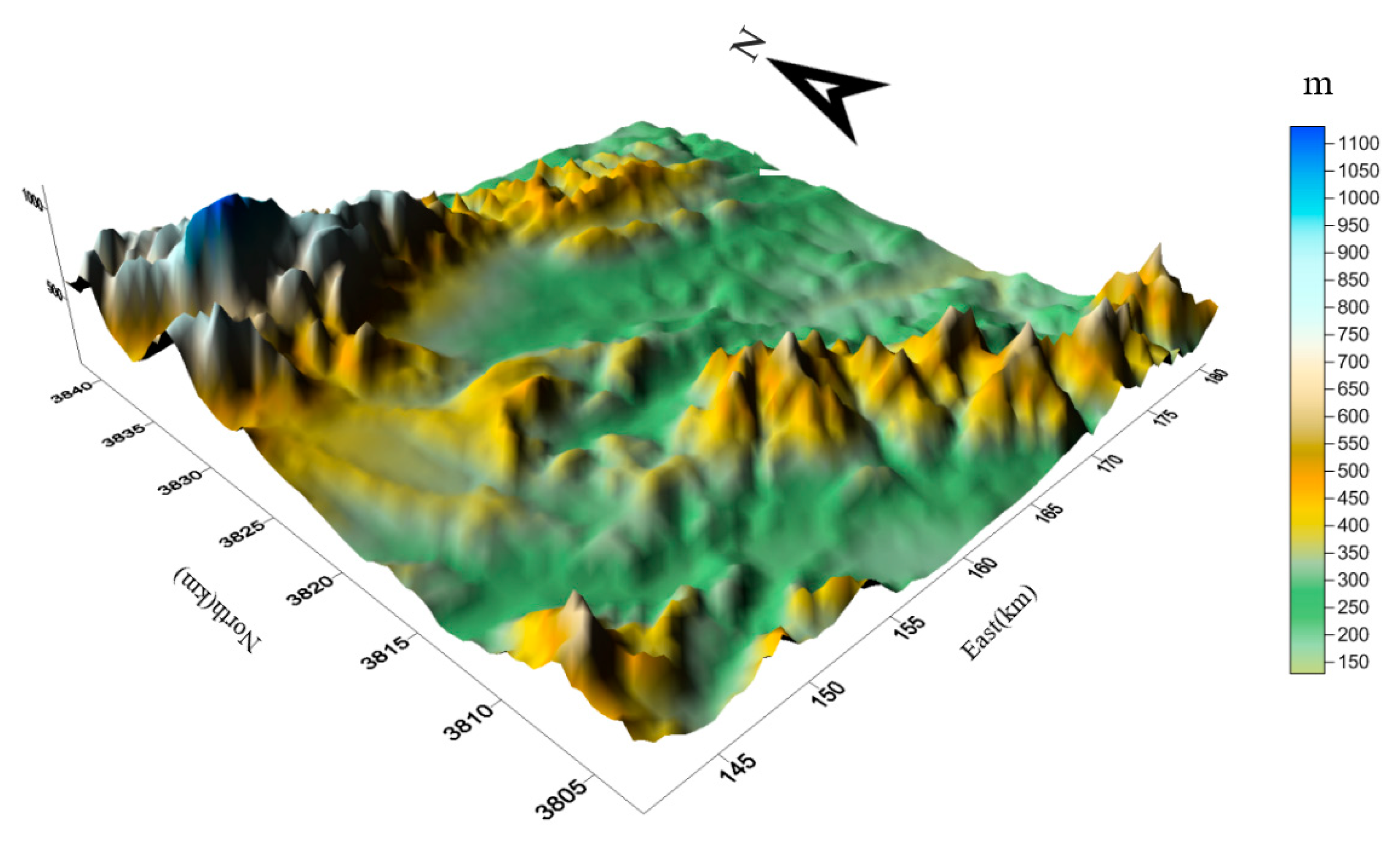
The data pre-processing module requires input of land use data, terrain elevation data, surface roughness, vegetation codes, and meteorological data from ground monitoring stations [36]. Geophysical data other than ground-based weather monitoring stations were downloaded from the CALPUFF model website (http://www.src.com/calpuff/data/ (accessed on 10 October 2019)). The terrain data downloaded in this study were obtained from the 3S Space Shuttle Radar Terrain Mapping File (STRM3) with a resolution of 90 m, and the terrain elevation data (TERREL.DAT) were processed by the terrain data pre-processing program (http://www.src.com/calpuff/data/terrain.html (accessed on 20 December 2019)). The land use data were obtained from the Asia portion of the USGS CLGC (the United States geological survey) database (https://earthexplorer.usgs.gov/ (accessed on 20 December 2019)) at a resolution of 1000 m and processed by the Land Use Data Preprocessing module to obtain gridded land use data (LU.DAT). The base time zone of the model was the eighth eastern region, the time step was 3600 s, and the chemical mechanism was the MESOPUFF II (the MESO scale puff) chemical mechanism [37]. The background concentration of ammonia was the default value, and the background concentration of ozone was the average of the ozone concentration data provided by the Zhengzhou Meteorological Monitoring Station, its latitude and longitude were 113.39° E and 34.43° N, respectively. This study only simulated the dry deposition processes from point sources and did not consider wet deposition. The three-dimensional topographic map of the study area is shown in Figure 2, which shows that the topography of the study area is high in the northwest, low in the southeast, and mountainous in the south and north, which is unfavorable to the transport and dispersion of pollutants. The central area is a hilly area, and the southeast and northeast sides of the terrain mat are relatively flat, which is favorable to the transport and diffusion of pollutants.
Meteorological data include ground monitoring station meteorological data and high-altitude meteorological data. The meteorological data of the ground monitoring station was derived from the 2018 continuous observations of the Zhengzhou Meteorological Station. The selected site is located inside the simulation domain of this study as its latitude and longitude were 113.39° E and 34.43° N, respectively, and thus it is reasonable to use the observed data from this station. The meteorological data mainly include wind direction, wind speed, temperature, and relative humidity. The CALPUFF model requires meteorological data in which ground meteorological data and altitude meteorological data were compulsory and rainfall data and surface station data were optional. In the simulation process of this study, rainfall and surface station data were not selected because wet deposition was not considered and domestic surface station data were missing. The initial meteorological field of the study area was generated using surface meteorological data, elevation data, and precipitation data simulated by the weather research and forecasting model (WRF) and then processed by the CALMET module because of the incomplete data from sounding weather stations near the study area. The WRF output data file format was converted to 3D.DAT file format by the CALWRF module [38]. The converted files extracted data on geopotential height, dew point, ground pressure, wind speed, sea level pressure, humidity, and surface temperature at each of the 27 altitude levels.
2.4. Emission Inventory Build Up
The activity level used to establish the emission inventory in this study was the production rate of brick and tile enterprises, and the data were obtained from the pollution source census data of Zhengzhou City. The emission factors were field research and test data, and two representative enterprises were selected as sampling points among 31 brick and tile enterprises in the study area to collect SO2, NOX, and PM2.5 emissions from the two enterprises. The concentrations of three pollutants, SO2, NOX, and PM2.5, emitted from the brick and tile industry in the study area were calculated and analyzed, and then the emission factors of pollutants from the brick and tile industry were calculated. The sampling instruments used for the particulate matter collection were the ELPI (electrical low-pressure impactor) particulate matter tester and the impactor MOUDI (microorifice uniform deposit impactor) manufactured by Dekati Company in Finland [39,40]. The calculation of PM2.5 concentration is shown in Equation (1), SO2 and NOX concentration is shown in Equation (2), and the calculation of emission factor is shown in Equation (3).
where, Ci denotes the mass concentration of PM2.5 emitted into the atmosphere in mg/m3; M2 denotes the mass of the membrane after sampling in g; M1 denotes the mass of the membrane before sampling in g; R denotes the dilution ratio; L denotes the flow rate of the sampler in L/min; t denotes the sample collection time in h. The sample is collected by the sample collector.
where, C2 denotes the baseline emission concentration of air pollutants in mg/m3; C1 denotes the measured emission concentration of air pollutants in the exhaust pipe in mg/m3; O1 denotes the measured value of oxygen content in dry flue gas in %; O denotes the baseline oxygen content in %.
where, EFi denotes emission factor, kg/t–product, kg/t–fuel, kg/t–raw material; Ci denotes pollutant concentration emitted into the atmosphere in mg/m3; Qi denotes average flue gas volume in the exhaust pipe in m3/h; t denotes sampling time in h; Mi denotes product output or fuel consumption during the sampling period in t or m3.
The localized emission factors were obtained from the measured sampling data and corresponding activity levels, and part of the measured emission factors were modified and extrapolated from the survey and online data. The selected localized emission factors are shown in Table 1, taking into account the actual situation of pollutant generation.
Through the enterprise data of the brick and tile industry to obtain the geographical location, raw material name and usage, fuel type and usage, product type and yield, control measures and efficiency of 31 enterprises, the emission factor method [41] was used to establish the emission inventory of the main pollutants SO2, NOX, and PM2.5 of the brick and tile industry in the study area in 2018, calculated as shown in Equation (4).
where, Ei denotes the emission of pollutant i in ton; Mj denotes the output of product j in ton; EFij denotes the emission factor of pollutant i when product j is produced in g/kg; and ηi denotes the overall efficiency of the pollution control measures for pollutant i in %.
3. Results
3.1. Emission Inventory
The SO2, NOX, and PM2.5 emissions from the brick and tile industry in the study area in 2018 were 564.86 tons, 513.16 tons, and 41.01 tons, respectively. The geographic location and spatial distribution of emissions of the 31 brick and tile enterprises in the study area are shown in Figure 3. From the figures, we can see that the distribution of the brick and tile enterprises was widely spread, and the enterprises with large pollutant emissions are located in the central part of the study area.
3.2. Model Validation
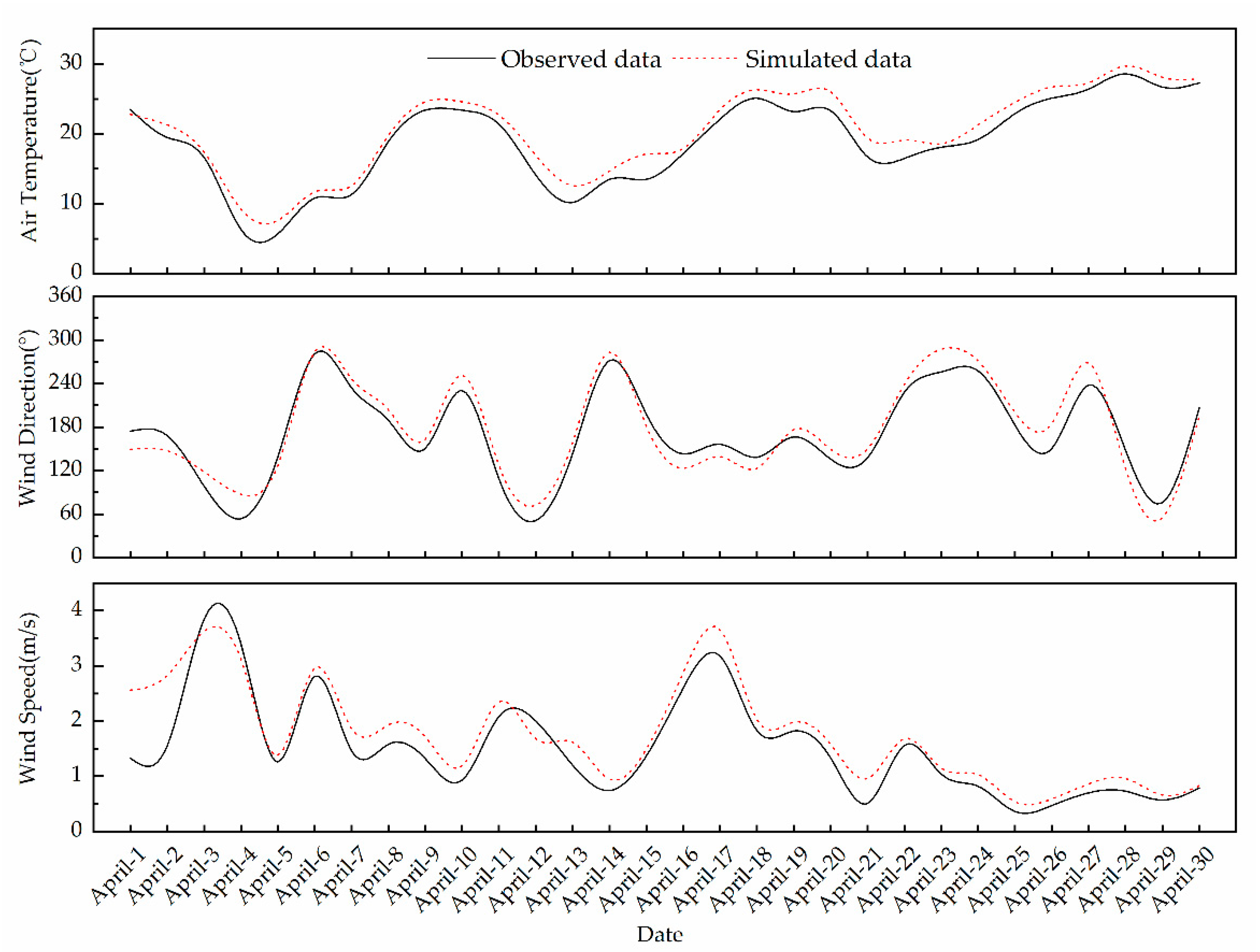
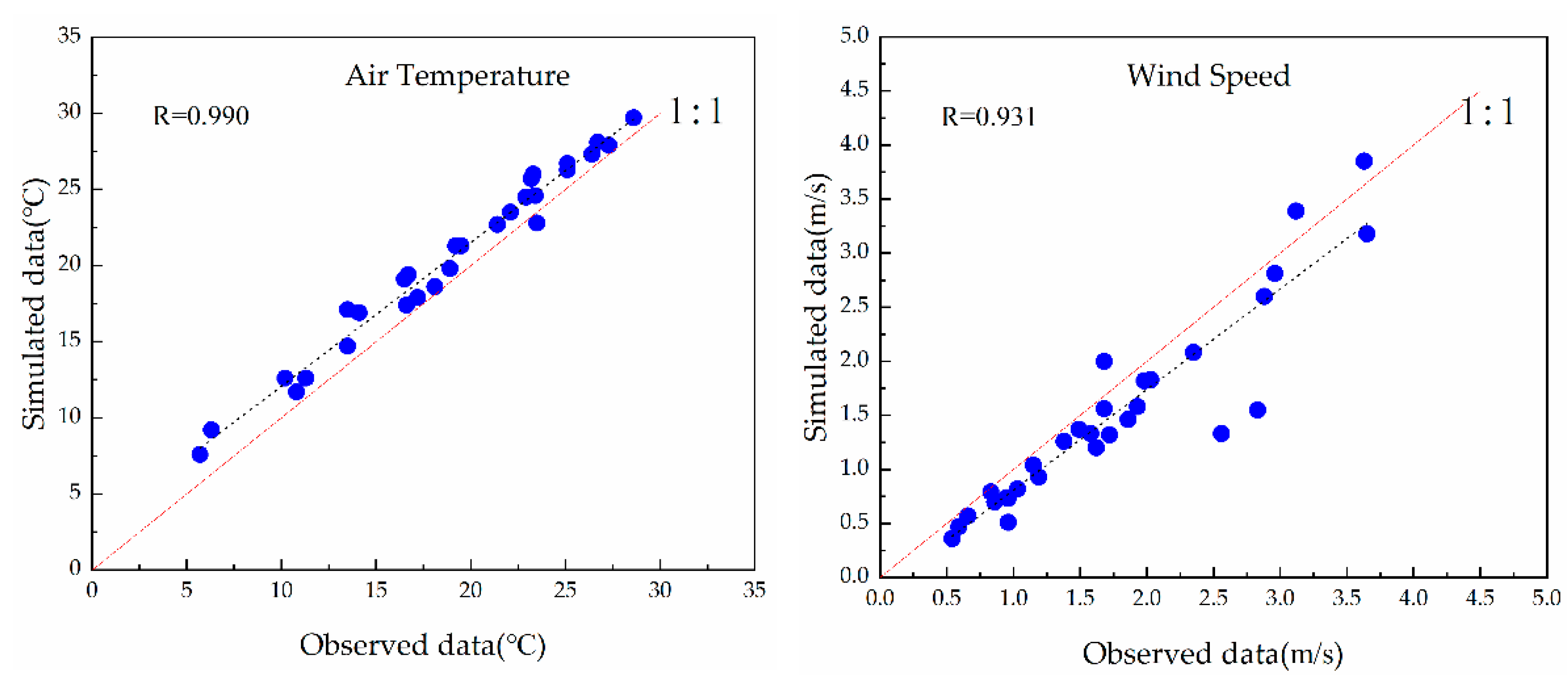
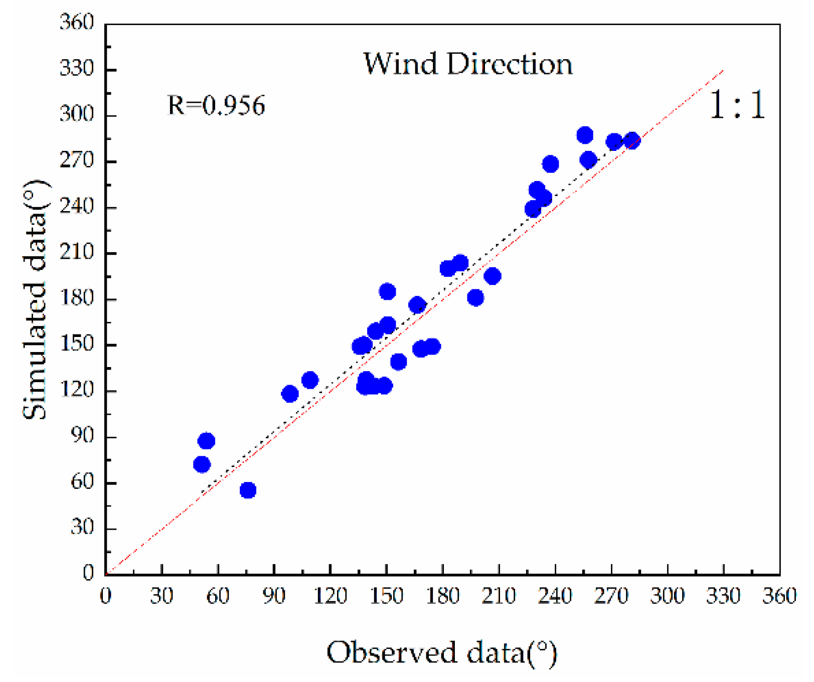
Simulation performance evaluation is a critical part of air quality modeling applications, and the correlation coefficient R can be used to assess the correlation between simulated and observed values [42]. This study validated the accuracy of the CALPUFF model using the atmospheric multi-pollutant emission inventory of the 2016 of Henan Province (Bai et al. [43]), as a baseline inventory. From the simulation results, we extracted the simulated meteorological variables of the Zhengzhou weather station, which is inside the study area, in April 2018 and their comparisons with the observed temperature, wind direction, and wind speed are shown in Figure 4. As can be seen from Figure 4, although there were some discrepancies between the simulated and observed values, the data differences were small, and their trends in time variation were almost the same. Figure 5 shows a scatter plot of simulated data versus observed data for air temperature, wind speed, and wind direction. From Figure 5, the correlation coefficients between the simulated and observed values of air temperature, wind speed, and wind direction are 0.990, 0.931, and 0.956, respectively. The independent samples t-test was performed on the simulated and observed values of air temperature, wind speed, and wind direction using SPSS (statistical program for social sciences, IBM) version 19. The t-test showed that the t-statistic for air temperature was 1.000, corresponding to a probability of 0.321, with a probability greater than the significance level of 0.05. The t-statistic for wind speed was 1.077, corresponding to a probability of 0.286, with a probability greater than the significance level of 0.05. The t-statistic for wind direction was 0.355, corresponding to a probability of 0.742, with a probability greater than the significance level of 0.05. There is no significant difference between the simulated and observed values of the three meteorological conditions. So, the CALMET model simulated meteorological field can meet the characteristics of the meteorological changes in the study area.
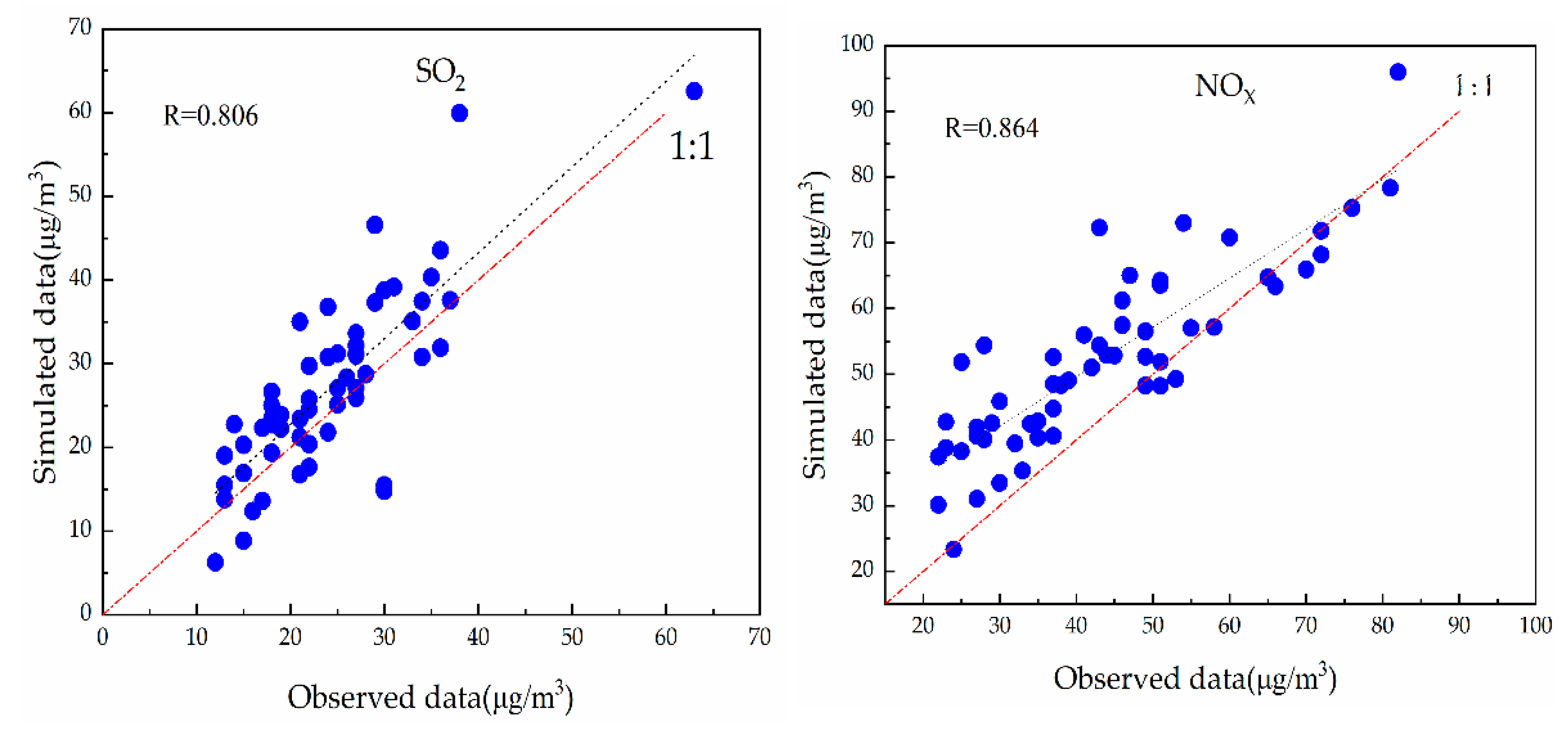
The air quality monitoring station at County Militia HQ with UTM coordinates of (165.95, 3829.16) km was selected as the source receptor site in the study area, and the daily average values of SO2, NOX, and PM2.5 concentrations from November to December 2018 of the monitoring station were compared with model outputs to validate the accuracy of the simulation results. As shown in Figure 6, the correlation coefficients of the SO2, NOX, and PM2.5 fit curves were 0.806, 0.864, and 0.875, respectively, indicating that the simulation fits well with observed data. The independent sample t-test was performed on the simulated and observed values of SO2, NOX, and PM2.5 using SPSS version 19. The t-test results showed that the t-statistic for SO2 was 1.563, corresponding to a probability of 0.121, with a probability greater than the significance level of 0.05. The t-statistic for NOX was 3.177, corresponding to a probability of 0.002, with a probability less than the significance level of 0.05. The t-statistic for PM2.5 was −2.747, corresponding to a probability of 0.015, with a probability less than the significance level of 0.05. The results show that the simulated values of SO2 are not significantly different from the observed values. While the simulated values of NOX and PM2.5 are somewhat different from the observed values, the differences are within the acceptable range with the mean simulated data for NOX being 20.5% higher than the mean observed data and the mean simulated data for PM2.5 being 21.8% lower than the mean observed data [9,44]. So, the CALPUFF model can be used to simulate the evolution of species concentrations emitted from brick and tile industry in the study area.
3.3. Meteorological Characterization
Xinmi city belongs to the northern temperate continental monsoon climate, and the monthly average temperature (T) variation in 2018 in the simulated area was obtained from the ground observed data of Xinmi meteorological monitoring station as shown in Table 2. The average monthly maximum temperature in the simulated range was 29.6 °C in July, the average monthly minimum temperature was 0.9 °C in January, and the average annual temperature was 16.2 °C in 2018. The average temperature of the four seasons varies significantly, with a large difference between winter and summer.
The average monthly and annual wind speed (WS) for 2018 in the simulated area obtained from the meteorological monitoring station is shown in Table 3, which shows that the lowest monthly average wind speed occurred in January with 1.29 m/s and the highest monthly average wind speed occurred in July with 2.03 m/s in the simulated area.
Using daily 24-h continuous wind direction and speed data from meteorological monitoring station for January, April, July, and October in 2018, a rose diagram of the simulated regional winds for all seasons was plotted, as shown in Figure 7. The dominant spring wind direction in the simulation area was between SSE-SE-ESE and WNW-WSW with a calculated average wind speed of 1.51 m/s; the dominant summer wind direction was between SSE-SE-ESE with a calculated average wind speed of 2.03 m/s; the dominant autumn wind direction was between WSW-WNW and SSE-SE-ESE with a calculated average wind speed of 1.44 m/s, and the dominant wind direction in winter was between WSW-WNW and NNE-NE-ENE, with a calculated average wind speed of 1.29 m/s. Wind speed was higher in spring and summer than in autumn and winter, and the dominant wind direction was the same in spring and summer, and the dominant wind direction was basically the same in autumn and winter, which was consistent with the temperate continental monsoon climate of Xinmi City. The wind speed in winter was obviously less than other seasons, and the low temperature leads to the lower boundary layer height (BLH), which is unfavorable to the dispersion of pollutants; while the high temperature in summer leads to the higher boundary layer height (BLH), which is more conducive to the diffusion of pollutants. Therefore, severe pollution is more likely to form in winter.
3.4. Air Pollutants Simulation Results
A total of 31 brick and tile enterprises were counted in the study area, and the impact of pollutant emissions from these brick and tile industries on the air quality of the study area was simulated based on the CALPUFF model using the 2018 brick and tile enterprise emission inventory estimated by the study as the baseline inventory. The hourly average concentrations of pollutants emitted by brick and tile enterprises in January, April, July, and October were obtained from the simulations.
3.4.1. SO2 Simulation Results
In terms of time, SO2 pollution had seasonal characteristics. The peak hourly average concentration was 156.32 μg/m3 in spring, 141.53 μg/m3 in summer, 186.54 μg/m3 in autumn, and 210.35 μg/m3 in winter, respectively, which meant that the peak hourly average concentration of SO2 in spring and summer was smaller than that in autumn and winter, and the peak hourly average concentration in winter was the highest. According to the ambient air quality (GB3095–2012), the primary concentration limit value of hourly average SO2 concentration is 150 μg/m3, which means that the peak hourly average SO2 concentration emitted by the brick and tile industry in autumn and winter of 2018 in the study area were 1.2 and 1.4 times higher than the primary concentration limit value, respectively.
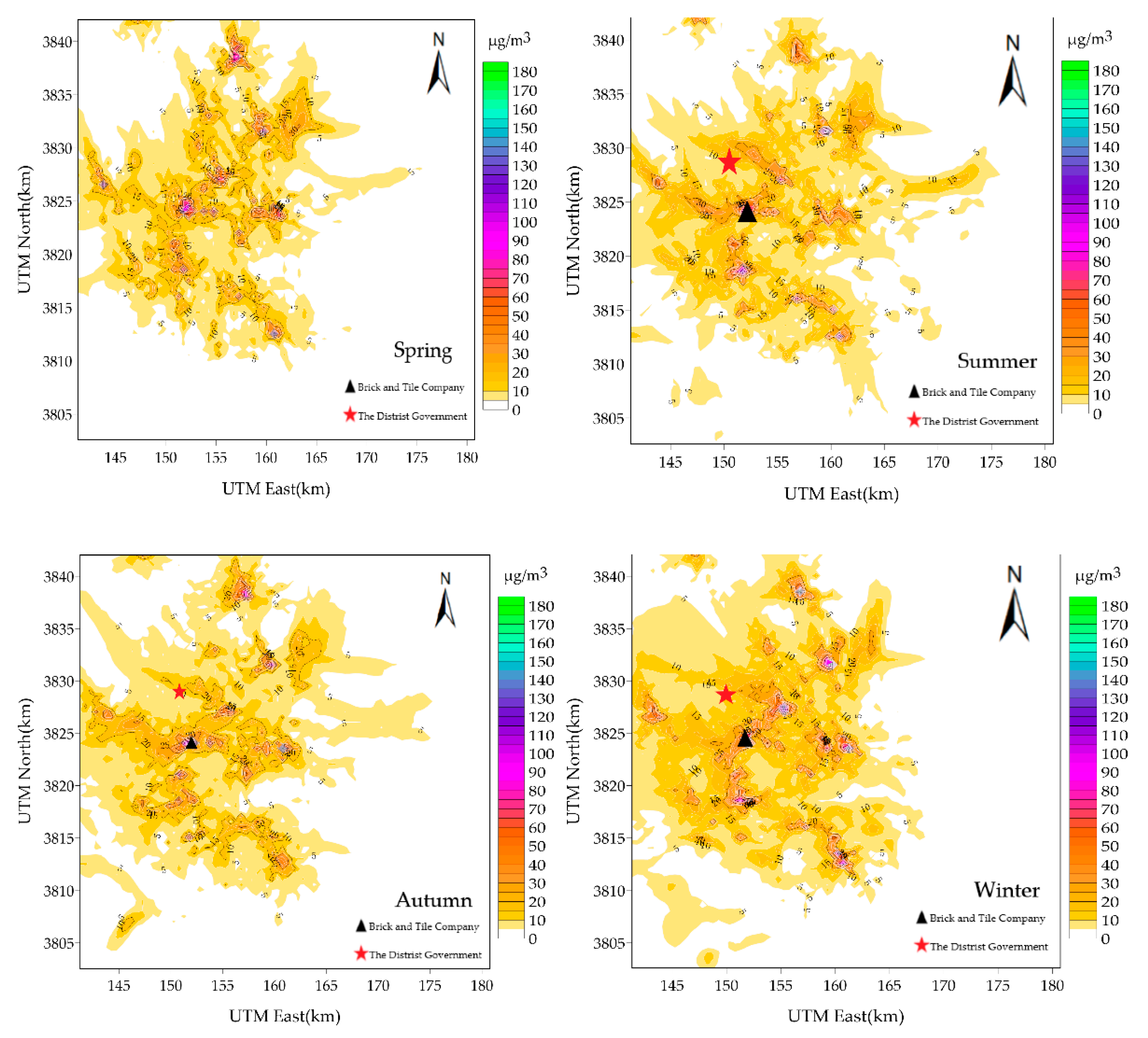
From the pollutant dispersion range, Figure 8 shows the contour map of hourly average concentration of SO2 based on the model simulation results. It can be seen that SO2 had a larger dispersion range in summer and a smaller dispersion range in autumn, winter, and spring. It was mainly due to the temperate continental monsoon climate of the study area, causing differences in average wind speed and direction among seasons. The meteorological data showed that the southeast and east winds predominated in the study area in summer, with an average wind speed of 2.03 m/s, which made SO2 diffuse to the west and northwest in summer, and due to the higher wind speed, the diffusion range was significantly large, and the concentration contour map showed that the SO2 concentration was still high in a range of about 10 km around the brick factory. While in autumn, winter, and spring, west, northeastern, and southeastern winds predominated, with average wind speeds of 1.44 m/s, 1.29 m/s, and 1.51 m/s, respectively, enabling SO2 to disperse along the downwind directions, but the dispersion range was smaller because of the lower wind speed.
3.4.2. NOX Simulation Results
On the basis of the model simulation results, the contour map of NOX four-season hourly average concentration was drawn, as shown in Figure 9. Combined with the three-dimensional topographic map of the study area (Figure 2), it can be seen that the NOX concentration distribution was basically the same as that of SO2, and points with higher pollutant concentrations were distributed in the basin-like area with lower topography in the middle and higher topography all around.
From the perspective of time variation, NOX pollution exhibited seasonal characteristics as well. The peak hourly average concentration of NOX was 142.42 μg/m3 in spring, 141.53 μg/m3 in summer, 167.65 μg/m3 in autumn, and 187.84 μg/m3 in winter, respectively. It is obvious that the concentration of NOX in spring and summer was lower than that in autumn and winter, and the peak hourly concentration in winter was the highest in all four seasons. It is worth mentioning that none of them exceeded the ambient air quality standard secondary concentration limit of 200 μg/m3.
3.4.3. PM2.5 Simulation Results
The hourly average concentration contour map of PM2.5 for four seasons drawn from the model simulation results was shown in Figure 10, and the pollution characteristics of PM2.5 were basically consistent with SO2 and NOX, indicating that the higher concentration points were also found in the high terrain around and low terrain in the middle. The peak hourly average concentration of PM2.5 was 12.80 μg/m3 in spring, 12.07 μg/m3 in summer, 13.39 μg/m3 in autumn, and 17.02 μg/m3 in winter, respectively. It is apparent that there was a relatively large increase in concentration in winter.
As far as the dispersion range is concerned, the dispersion distance of PM2.5 was relatively small compared with that of SO2 and NOX. In addition, the diffusion range was larger in summer due to wind speed, smaller in spring and autumn, and smallest in winter due to counter-temperature phenomenon and low wind speed.
4. Discussion
4.1. Analysis of Simulation Results
From Section 3.4, the concentration changes of all three pollutants were characterized by seasonality. The pollutants’ diffusion range was large, and the pollutants’ concentration was the lowest in summer, while the pollutants’ concentration was the highest in winter when the diffusion range was small. This is related to the meteorological factors in the study area, where high average wind speed and high average temperature in summer were beneficial to the diffusion of pollutants, thus resulting in low pollutant concentrations; while low average wind speed and low average temperature in winter were prone to inversion, which was unfavorable to the diffusion of pollutants, resulting in high pollutant concentrations.
Combining the contour map of hourly average pollutant concentrations in the study area and the three-dimensional topographic map (Figure 2), it can be seen that most of the points with high pollutant concentrations were located at lower terrain, which was related to the location of the brick and tile enterprises and the topography of the study area. Due to the high topography and poor air flow ability around the enterprises, it was easy to cause the accumulation of pollutants. The eastern part of the study area is flat, which was helpful for the diffusion of pollutants, and the brick and tile enterprises caused less pollution to this part of the area. While for the central and western parts of the area, the pollution caused was more serious because of the large number of enterprises in this part of the area, the large amount of pollutant emissions, and the high terrain around the enterprises.
Therefore, in order to avoid the accumulation of pollutants, brick and tile enterprises should take into account factors such as topography and meteorology to choose suitable plant sites.
4.2. Analysis of the Impact of Local Emission on Air Quality
The Ambient Air Quality Standard (GB3095–2012) stipulates that the 24 h average concentration secondary limits for SO2, NOX, and PM2.5 were 150 μg/m3, 100 μg/m3, and 75 μg/m3, respectively. The 24-h average concentration peaks and rates of contribution to the 24-h average concentration secondary limits of pollutants simulated by the CALPUFF model for different seasons were shown in Table 4. As shown in Table 4, the 24-h average concentration peak of SO2 in winter was 50.36 μg/m3, much higher than that in spring, summer, and autumn. The 24-h average concentration peak of NOx in winter was 45.04 μg/m3, much higher than that in spring, summer, and autumn. The 24-h average concentration peaks of PM2.5 in the four seasons were more or less similar, but it was the largest in winter at 3.24 μg/m3. As a result, brick and tile enterprises emit the highest concentration of pollutants in winter. The rates of contribution to the 24-h average concentration secondary limits of the 24-h average peak concentration of the three pollutants were the highest in winter, the second highest in autumn, and the lowest in summer. Among the three pollutants, NOX had the highest rates of contribution to secondary standard concentration limit value with 45.0% in winter, SO2 ranked second at 33.6%, and PM2.5 had the lowest of 4.3%.
The Xinmi Housing Management Office monitoring station was selected as pollutant receptor site, and the observed monthly average concentrations in winter were compared with the monthly average concentration simulated by the model, as shown in Table 5. The monthly average concentration of SO2 in winter at the monitoring station of housing management was 46.32 μg/m3, with a simulated value of 3.05 μg/m3 and a contribution of 6.58%; the monthly average concentration of NOX was 53.52 μg/m3, with a simulated value of 2.88 μg/m3 and a contribution of 5.38%; and the monthly average concentration of PM2.5 was 72.34 μg/m3, with a simulated value of 1.03 μg/m3 and a contribution of 1.42%.
Due to the lack of literature results of the brick and tile industry simulation studies, we compared the results with the simulation analysis of the Beijing-Tianjin-Hebei thermal power industry by the group of Box in [1]. The result showed that the maximum contribution concentration of the thermal power industry to the background concentration ranged from 1.92% to 6.85%, which was comparatively close to the results of this study.
4.3. Emission Control Measures
From Section 4.2, due to meteorological factors and topographical features, the impact of pollutant emissions from the brick and tile industry on air pollution in the region was seasonal, with winter being the most polluted of the four seasons. Among the three main pollutants emitted by the brick and tile industry, SO2 and NOX emissions contributed a high proportion to the local air quality concentration, which was caused by the fact that the raw materials of the brick and tile industry were mainly coal gangue containing a large amount of sulfur, and the enterprises lacked adequate and effective SO2 and NOX control facilities.
Therefore, our recommendations are as follows:
- (1)
- The brick and tile industry should strictly control and strengthen the governance of raw fuel crushing, drying and roasting, preparation and molding, and other stages of disorganized emission of smoke and powder dust. It should be equipped with de-dusting facilities in each link of the production process. In addition, it should develop and promote the comprehensive treatment technology and equipment for flue gas desulfurization, de-nitration, and de-dusting of brick and tile kilns.
- (2)
- Sintered brick kilns using coal, coal gangue, and other fuels should be sealed to store fuel and take measures such as windproof, dust suppression, and dust reduction.
- (3)
- Sintered brick kilns should be installed with automatic pollutant monitoring facilities. The installation of distributed control systems (DCS) shall be promoted to record the main parameters of the operation of environmental protection facilities and related production processes of industrial furnaces and kilns, so as to achieve real-time visualization and management through online monitoring systems to ensure compliance with the emission standards.
4.4. Significance and Limitations
The brick and tile industry, as a typical industrial furnace and kiln industry, has been studied mostly in terms of pollutant emission characteristics, source profiles, emission factors, and emission inventories. This study not only established a source emission inventory, but also simulated the impact of pollutants emitted from the brick industry on air quality by combining the CALPUFF model. Moreover, the source emission inventory in this study was based on the 2018 Zhengzhou City Pollution Source Census data, combining online data and field survey data, which is more detailed and accurate than the data collected in previous industrial emission inventories, thus improving the resolution of the source emission inventory.
Inevitably, there are still some limitations of this study due to limited data availability and other limitations. Firstly, when selecting representative enterprises for sampling, the enterprise information obtained was incomplete, which may cause some uncertainties in the emission inventory. In addition, the relatively small number of source monitoring points set up in the study area did not allow for full assessment of the source concentrations at the simulated sensitive sites. For this reason, as much valid business information as possible should be collected, and additional source monitoring points should be set up at the location of the sensitive sites in future studies.
Nonetheless, this study can still provide some guidance on the management of air pollutants in the brick and tile industry in Xinmi City and other areas with similar characteristics.
5. Conclusions
The meteorological data from the Zhengzhou meteorological monitoring station and the pollutant observed data from the Xinmi City air quality monitoring station were compared with the corresponding simulated data to evaluate the accuracy of the simulated meteorological field and pollutant concentration changes by the CALPUFF model. The results showed that the meteorological field simulated by the CALMET model could meet the meteorological conditions for pollutant concentration simulation in the study area; the correlation coefficient between the simulated pollutant concentrations and the observed concentration changes fit curve of the CALPUFF model was greater than 0.8, and there is no significant difference between the simulated data and the observed data for SO2, and the difference between the values of NOX and PM2.5 is within the acceptable range. The model can well reproduce the impact of industrial point sources on air quality.
The hourly average concentrations of SO2, NOX, and PM2.5 obtained from model simulations in spring, summer, autumn, and winter were analyzed, and the spatial and temporal distribution of the three pollutants in the study area was discussed. The simulated concentrations showed seasonal characteristics, with a large pollutant dispersion range in summer, smaller in winter, and more severe pollution in winter than in other seasons. The brick and tile industry had a greater impact on the pollution in the west-central part of the study area.
The peak concentrations of the three pollutants in different seasons were the highest in winter. In winter, NOX accounted for the highest percentage of the limits value of standard, accounting for 45.0%; SO2 followed, accounting for 33.6%; PM2.5 was the lowest, accounting for 4.3%. Comparing the monthly average concentration observed value of three pollutants in winter with the simulated value of Xinmi City Housing Authority Monitoring Station as the receptor point, it can be seen that SO2 and NOX had higher contributions to the atmospheric concentration of the study area, with a contribution rate of 6.58% and 5.38%, respectively; PM2.5 had the lowest contribution rate of 1.42%. Therefore, SO2 and NOx in the brick and tile industry in Xinmi City had greater potential for emission reduction, and the emission control of SO2 and NOX should be strengthened.
Author Contributions
Conceptualization, Q.X. and L.X.; methodology, L.X. and Q.X.; software, L.X., R.H. and Q.X.; validation, L.X. and R.H.; formal analysis, L.X. and Q.X.; investigation, R.H.; writing—original draft preparation, L.X.; writing—review and editing, Q.X., R.H. and L.X.; visualization, L.X.; supervision, Q.X. All authors have read and agreed to the published version of the manuscript.
Funding
This research was funded by the National Key Research and Development Program (grant number 2017YFC0212400).
Institutional Review Board Statement
Not applicable.
Informed Consent Statement
Not applicable.
Data Availability Statement
The data presented in this study are available on request from the corresponding author. The data are not publicly available due to the supporting project for this study has not yet been finished and the data cannot be made public at this time.
Acknowledgments
We would like to thank the Institute of Environmental Science, Zhengzhou University, for providing the experimental platform.
Conflicts of Interest
The authors declare no conflict of interest.
References
- Bo, X.; Wang, G.; Wen, R.; Heng, Y.J.; Ding, F.; Wu, C.Z. Air pollution effect of the thermal power plants in Beijing-Tianjin-Hebei region. China Environ. Sci. 2015, 35, 364–373. [Google Scholar]
- Gong, Z.X.; Geng, H.; Zhang, J.H.; Zhou, H.; Peng, Y.; Zhai, S.Y. Ecological and health risks of trace heavy metals in atmospheric PM2.5 collected in Wuxiang Town, Shanxi Province. Environ. Sci. 2018, 39, 1004–1013. [Google Scholar] [CrossRef]
- Xu, W.J.; Zeng, Z.T.; Xu, Z.Y.; Li, X.D.; Chen, X.W.; Li, X. Public health benefits of optimizing urban industrial land layout—The case of Changsha, China. Environ. Pollut. 2020, 263, 114388. [Google Scholar] [CrossRef] [PubMed]
- Guo, J.; Li, L.; Wu, X.C.; Zhuang, C.; Liu, S.J.; Huang, X.J. Simulation study on the effect of key industrial sources on air quality in winter heavy pollution process in Jinan. Acta Sci. Circumstantiae 2019, 39, 134–142. [Google Scholar] [CrossRef]
- Zhou, X. Promoting air pollution control in the brick and tile industry. Brick Mortar World 2018, 14, 15–17. [Google Scholar]
- Sirithian, D.; Thepanondh, S.; Laowagul, W.; Morknoy, D. Atmospheric dispersion of polycyclic aromatic hydrocarbons from open burning of agricultural residues in Chiang Rai, Thailand. Air Qual. Atmos. Health 2017, 10, 861–871. [Google Scholar] [CrossRef]
- Levy, J.I.; Spengler, J.D.; Hlinka, D.; Sullivan, D.; Moon, D. Using CALPUFF to evaluate the impacts of power plant emissions in Illinois: Model sensitivity and implications. Atmos. Environ. 2002, 36, 1063–1075. [Google Scholar] [CrossRef]
- Bo, X.; Ding, F.; Xu, H.; Li, S.B. Review of atmospheric diffusion spersion model CALPUFF technology. Adm. Tech. Environ. Monit. 2009, 21, 9–13. [Google Scholar]
- Holnicki, P.; Kaluszko, A.; Trapp, W. An urban scale application and validation of the CALPUFF model. Atmos. Pollut. Res. 2016, 7, 393–402. [Google Scholar] [CrossRef]
- Lee, H.D.; Yoo, J.W.; Kang, M.K.; Kang, J.S.; Jung, J.H.; Oh, K.J. Evaluation of concentrations and source contribution of PM10 and SO2 emitted from industrial complexes in Ulsan, Korea: Interfacing of the WRF–CALPUFF modeling tools. Atmos. Pollut. Res. 2014, 5, 664–676. [Google Scholar] [CrossRef] [Green Version]
- Abdul-Wahab, S.; Sappurd, A.; Al-Damkhi, A. Application of California Puff (CALPUFF) model: A case study for Oman. Clean Technol. Environ. Policy 2011, 13, 177–189. [Google Scholar] [CrossRef]
- Ghannam, K.; El-Fadel, M. Emissions characterization and regulatory compliance at an industrial complex: An integrated MM5/CALPUFF approach. Atmos. Environ. 2013, 69, 156–169. [Google Scholar] [CrossRef]
- Ren, Y.J.; Lai, W.A.; Gao, Q.X. Numerical simulation of air environment of Yangquan, Shanxi Province. Environ. Sci. Technol. 2010, 33, 174–180. [Google Scholar] [CrossRef]
- Ma, Y.; Bo, X.; Gao, S.; Cheng, G.Q.; Li, S.B.; Li, G. Study on atmospheric environmental impact of key industries in urban areas of Cangzhou, Hebei Province. Environ. Impact Assess. 2019, 41, 16–19. [Google Scholar] [CrossRef]
- Mao, H.M.; Zhang, K.S.; Di, B.F.; Yang, M.M.; Ma, S. The high-resolution temporal and spatial allocation of emission inventory for Chengdu. Acta Sci. Circumstantiae 2017, 37, 23–33. [Google Scholar] [CrossRef]
- Pretorius, I.; Piketh, S.; Burger, R. Emissions management and health exposure: Should all power stations be treated equal? Air Qual. Atmos. Health 2017, 10, 509–520. [Google Scholar] [CrossRef]
- Xu, Y.F.; Qu, S.; Yan, J.; Song, G.W.; Zhong, L.H. Development of an Air Pollutant emission inventory of cement industry for Beijing and pollution characteristics analysis. Environ. Sci. Technol. 2014, 37, 201–204. [Google Scholar] [CrossRef]
- Whiteman, C.D.; Hoch, S.W.; Horel, J.D.; Charland, A. Relationship between particulate air pollution and meteorological variables in Utah’s Salt Lake Valley. Atmos. Environ. 2014, 94, 742–753. [Google Scholar] [CrossRef]
- Bares, R.; Lin, J.C.; Hoch, S.W.; Baasandorj, M.; Mendoza, D.L.; Fasoli, B. The Wintertime Covariation of CO2 and Criteria Pollutants in an Urban Valley of the Western United States. J. Geophys. Res. Atmos. 2018, 123, 2684–2703. [Google Scholar] [CrossRef]
- Nidzgorska-Lencewicz, J.; Czarnecka, M. Thermal Inversion and Particulate Matter Concentration in Wrocław in Winter Season. Atmosphere 2020, 11, 1351. [Google Scholar] [CrossRef]
- Bo, X.; Wu, Z.X.; Wang, G.; Hu, C.J.; Ding, F.; Wu, C.Z. Study on the standardized application of CALPUFF model. Environ. Sci. Technol. 2014, 37, 530–534. [Google Scholar] [CrossRef]
- Ren, Z.; Ma, H.T.; Wang, L.; Yang, X.L. Using CALPUFF in atmospheric prediction and environmental capacity calculation. Environ. Sci. Technol. 2011, 34, 201–205. [Google Scholar] [CrossRef]
- Cui, H.L.; Yao, R.T.; Xu, X.J.; Xin, C.T.; Yang, J.M. A tracer experiment study to evaluate the CALPUFF real time application in a near-field complex terrain setting. Atmos. Environ. 2011, 45, 7525–7532. [Google Scholar] [CrossRef]
- Otero-Pregigueiro, D.; Fernandez-Olmo, I. Use of CALPUFF to predict airborne Mn levels at schools in an urban area impacted by a nearby manganese alloy plant. Environ. Int. 2018, 119, 455–465. [Google Scholar] [CrossRef] [PubMed]
- Rzeszutek, M. Parameterization and evaluation of the CALMET/CALPUFF model system in near-field and complex terrain—Terrain data, grid resolution and terrain adjustment method. Sci. Total Environ. 2019, 689, 31–46. [Google Scholar] [CrossRef]
- Ghannam, K.; El-Fadel, M. A framework for emissions source apportionment in industrial areas: MM5/CALPUFF in a near-field application. J. Air Waste Manag. Assoc. 2013, 63, 190–204. [Google Scholar] [CrossRef] [Green Version]
- Weng, J.S. The application and comparison of ISC3 and CALPUFF model. Environ. Sci. Technol. 2012, 25, 52–54. [Google Scholar]
- Guo, D.P.; Wang, R.; Zhao, P. Spatial distribution and source contributions of PM2.5 concentrations in Jincheng, China. Atmos. Pollut. Res. 2020, 11, 1281–1289. [Google Scholar] [CrossRef]
- Li, S.Y.; Xie, S.D. Spatial distribution and source analysis of SO2 concentration in Urumqi. Int. J. Hydrog. Energy 2016, 41, 15899–15908. [Google Scholar] [CrossRef]
- Tian, F.; Bo, X.; Xue, X.D.; Jia, Y.T.; Tang, Q.H.; Sun, H.T. Study on settlement of dioxin pollutants under complex terrain-weather conditions. China Environ. Sci. 2019, 39, 1678–1686. [Google Scholar] [CrossRef]
- Cui, H.L.; Yao, R.T.; Chen, L.Q.; Lv, M.H.; Xin, C.T.; Wu, Q. Field study of atmospheric boundary layer observation in a hilly Gobi Desert region and comparison with the CALMET/CALPUFF model. Atmos. Environ. 2020, 235, 13. [Google Scholar] [CrossRef]
- Wang, Y.; Li, Y.; Qiao, Z.; Lu, Y.L. Atmospheric transmission rule on air pollution in Beijing-Tianjin-Hebei urban agglomeration: A comparative analysis of two emission inventories. China Environ. Sci. 2019, 39, 4561–4569. [Google Scholar] [CrossRef]
- Akyuz, E.; Kaynak, B. Use of dispersion model and satellite SO2 retrievals for environmental impact assessment of coal-fired power plants. Sci. Total Environ. 2019, 689, 808–819. [Google Scholar] [CrossRef] [PubMed]
- Chen, J.S.; Bo, X.; Xu, J.F.; Kan, H.; Wu, P.C.; Qu, J.B. Research progress on VOCs simulationg in environmental impact assessment in China. Environ. Eng. 2018, 36, 143–147. [Google Scholar] [CrossRef]
- Ma, Y.L.; Wang, S.S.; Wang, K.; Liu, L.; Zhang, R.Q. Co-benefits analysis of energy cascade utilization in an industrial park in China. Environ. Sci. Pollut. Res. Int. 2019, 26, 16181–16194. [Google Scholar] [CrossRef] [PubMed]
- Lu, Y.Y.; Sun, W.; Deng, H.Q.; He, D.Y. Characteristics and simulation of atmospheric NO2 concentration in winter of Hefei City. Environ. Sci. Technol. 2017, 40, 124–130. [Google Scholar] [CrossRef]
- Scire, J.S.; Strimaitis, D.G.; Yamartino, R.J. A User‘s Guide for the CALPUFF Dispersion Model (Version 5); Earth Tech Inc.: Concord, MA, USA, 2000; Volume 521, pp. 1–521. [Google Scholar]
- Kan, H.; Bo, X.; Qu, J.B.; Yang, Z.X.; Wu, P.C.; Tian, F. Air quality impacts of power plant emissions in Hainan Province, 2015. China Environ. Sci. 2019, 39, 428–439. [Google Scholar] [CrossRef]
- Sui, Z.F.; Zhang, Y.S.; Peng, Y.; Norris, P.; Cao, Y.; Pan, W.P. Fine particulate matter emission and size distribution characteristics in an ultra-low emission power plant. Fuel 2016, 185, 863–871. [Google Scholar] [CrossRef]
- Peng, Y.; Sui, Z.F.; Zhang, Y.S.; Wang, T.; Norris, P.; Pan, W.P. The effect of moisture on particulate matter measurements in an ultra-low emission power plant. Fuel 2019, 238, 430–439. [Google Scholar] [CrossRef]
- Ding, Q.Q.; Wei, W.; Shen, Q.; Sun, Y.H. Major air pollutant emissions of coal-fired power plant in Yangtze River Delta. Environ. Sci. 2015, 36, 2389–2394. [Google Scholar] [CrossRef]
- Xu, W.B.; Xu, Y.L.; Wang, J.N.; Tang, X.L. Ambient air quality impact of emissions from thermal power industry. China Environ. Sci. 2016, 36, 1281–1288. [Google Scholar]
- Bai, L.; Lu, X.; Yin, S.S.; Zhang, H.; Ma, S.L.; Wang, C. A recent emission inventory of multiple air pollutant, PM2.5 chemical species and its spatial-temporal characteristics in central China. J. Clean. Prod. 2020, 269, 122114. [Google Scholar] [CrossRef]
- Oshan, R.; Kumar, A.; Masuraha, A. Application of the USEPA’s CALPUFF model to an urban area. Environ. Prog. 2006, 25, 12–17. [Google Scholar] [CrossRef]
Figure 1.
Geographical location of the studied area.

Figure 2.
Three-dimensional topographic map of the studied area.

Figure 3.
Location distribution of brick and tile enterprises and distribution of pollutant emissions (a) SO2, (b) NOX, (c) PM2.5.
Figure 3.
Location distribution of brick and tile enterprises and distribution of pollutant emissions (a) SO2, (b) NOX, (c) PM2.5.

Figure 4.
Meteorological factors temperature, wind speed, wind direction.

Figure 5.
Scatter plot of simulated versus observed data for air temperature, wind speed, and wind direction.
Figure 5.
Scatter plot of simulated versus observed data for air temperature, wind speed, and wind direction.


Figure 6.
Scatter plots of simulated and observed concentrations of three pollutants, SO2, NOX, and PM2.5 at the County Militia HQ.
Figure 6.
Scatter plots of simulated and observed concentrations of three pollutants, SO2, NOX, and PM2.5 at the County Militia HQ.


Figure 7.
Wind rose chart of the study area for different seasons in 2018.

Figure 8.
Contours of the hourly average concentration of SO2 in spring, summer, autumn, and winter.
Figure 8.
Contours of the hourly average concentration of SO2 in spring, summer, autumn, and winter.

Figure 9.
Contour map of hourly average concentration of NOX in spring, summer, autumn, and winter.

Figure 10.
The contour map of the hourly average concentration of PM2.5 in spring, summer, autumn, and winter.
Figure 10.
The contour map of the hourly average concentration of PM2.5 in spring, summer, autumn, and winter.


Table 1.
Localized emission factors for the brick and tile industry.
| Type of Product | Raw Material | Emission Factor | Unit | ||
|---|---|---|---|---|---|
| PM2.5 | SO2 | NOX | |||
| Coal gangue brick | Coal gangue, sludge, etc. | 0.140 | 34.856 | 7.148 | kg/10,000 standard bricks |
| Baked brick | Shale, fly ash, etc. | 0.033 | 0.948 | 2.016 | kg/10,000 standard bricks |
Table 2.
Average monthly temperature in the simulation area for 2018.
| Month | January | February | March | April | May | June | July | August | September | October | November | December | Annual |
|---|---|---|---|---|---|---|---|---|---|---|---|---|---|
| T (℃) | 0.9 | 3.6 | 9.2 | 19.1 | 23.4 | 26.7 | 29.6 | 27.9 | 23.4 | 18.1 | 9.1 | 3.2 | 16.2 |
Table 3.
Average monthly wind speed in the simulation area for 2018.
| Month | January | February | March | April | May | June | July | August | September | October | November | December | Annual |
|---|---|---|---|---|---|---|---|---|---|---|---|---|---|
| WS (m/s) | 1.29 | 1.36 | 1.49 | 1.51 | 1.47 | 1.83 | 2.03 | 1.76 | 1.53 | 1.44 | 1.39 | 1.31 | 1.54 |
Table 4.
The average concentration peak of pollutants in different seasons in 24 h and the rate of standard occupation.
Table 4.
The average concentration peak of pollutants in different seasons in 24 h and the rate of standard occupation.
| Season | SO2 | NOX | PM2.5 | ||||||
|---|---|---|---|---|---|---|---|---|---|
| Ci (μg/m3) | Cstandard (μg/m3) | Ratio to Standard Value (%) | Ci (μg/m3) | Cstandard (μg/m3) | Ratio to Standard Value (%) | Ci (μg/m3) | Cstandard (μg/m3) | Ratio to Standard Value (%) | |
| Spring | 37.90 | 150 | 25.3 | 34.07 | 100 | 34.1 | 2.39 | 75 | 3.2 |
| Summer | 35.18 | 150 | 23.5 | 33.06 | 100 | 33.1 | 2.28 | 75 | 3.0 |
| Autumn | 38.62 | 150 | 25.7 | 34.55 | 100 | 34.5 | 2.73 | 75 | 3.6 |
| Winter | 50.36 | 150 | 33.6 | 45.04 | 100 | 45.0 | 3.24 | 75 | 4.3 |
Note: Ci (μg/m3) represents the 24-h average concentration peak; Cstandard (μg/m3) represents the secondary standard concentration limit value.
Table 5.
Comparison of simulated and observed concentrations in brick and tile industry.
| Pollutants | Monthly Average of Simulated Concentrations (μg/m3) | Monthly Average of Observed Concentrations (μg/m3) | Ratio of Simulated to Observed Values (%) |
|---|---|---|---|
| SO2 | 3.05 | 46.32 | 6.58 |
| NOX | 2.88 | 53.52 | 5.38 |
| PM2.5 | 1.03 | 72.34 | 1.42 |
Publisher’s Note: MDPI stays neutral with regard to jurisdictional claims in published maps and institutional affiliations. |
© 2021 by the authors. Licensee MDPI, Basel, Switzerland. This article is an open access article distributed under the terms and conditions of the Creative Commons Attribution (CC BY) license (http://creativecommons.org/licenses/by/4.0/).
Share and Cite
MDPI and ACS Style
Xie, L.; Xu, Q.; He, R. Atmospheric Pollution Impact Assessment of Brick and Tile Industry: A Case Study of Xinmi City in Zhengzhou, China. Sustainability 2021, 13, 2414. https://0-doi-org.brum.beds.ac.uk/10.3390/su13042414
AMA Style
Xie L, Xu Q, He R. Atmospheric Pollution Impact Assessment of Brick and Tile Industry: A Case Study of Xinmi City in Zhengzhou, China. Sustainability. 2021; 13(4):2414. https://0-doi-org.brum.beds.ac.uk/10.3390/su13042414
Chicago/Turabian StyleXie, Liuzhen, Qixiang Xu, and Ruidong He. 2021. "Atmospheric Pollution Impact Assessment of Brick and Tile Industry: A Case Study of Xinmi City in Zhengzhou, China" Sustainability 13, no. 4: 2414. https://0-doi-org.brum.beds.ac.uk/10.3390/su13042414
Note that from the first issue of 2016, this journal uses article numbers instead of page numbers. See further details here.