
Aiming Strategy on a Prototype-Scale Solar Receiver: Coupling of Tabu Search, Ray-Tracing and Thermal Models

Processes, Materials and Solar Energy Laboratory, CNRS-PROMES (UPR 8521), 66120 Font-Romeu Odeillo, France
*
Author to whom correspondence should be addressed.
Sustainability 2021, 13(7), 3920; https://0-doi-org.brum.beds.ac.uk/10.3390/su13073920
Submission received: 10 February 2021
/
Revised: 25 March 2021
/
Accepted: 27 March 2021
/
Published: 1 April 2021
(This article belongs to the Special Issue Advances in Solar Thermal Energy)
Abstract
:An aiming point strategy applied to a prototype-scale power tower is analyzed in this paper to define the operation conditions and to preserve the lifetime of the solar receiver developed in the framework of the Next-commercial solar power (CSP) H2020 project. This innovative solar receiver involves the fluidized particle-in-tube concept. The aiming solution is compared to the case without the aiming strategy. Due to the complex tubular geometry of the receiver, results of the Tabu search for the aiming point strategy are combined with a ray-tracing software, and these results are then coupled with a simplified thermal model of the receiver to evaluate its performance. Daily and hourly aiming strategies are compared, and different objective normalized flux distributions are applied to quantify their influence on the receiver wall temperature distribution, thermal efficiency and particle outlet temperature. A gradual increase in the solar incident power on the receiver is analyzed in order to keep a uniform outlet particle temperature during the start-up. Results show that a tradeoff must be respected between wall temperature and particle outlet temperature.
1. Introduction
In all commercial solar power tower plants (CSP tower), the solar receiver is a major component, since it reaches the highest wall temperature of the solar loop. An Aiming Point Strategy (APS) is crucial to avoid any deterioration of the receiver due to uneven flux distribution leading to hot spots and strong thermal stresses [1]. APS limits the maximum flux density and distributes the flux more evenly on the receiver surface. These strategies are complex because, while avoiding the appearance of hot spots and preserving the lifetime of the receiver [2], the receiver size must be minimized for cost reasons and the spillage losses (part of the concentrated solar radiation that does not cross the receiver aperture) must be reduced to ensure a high overall optical efficiency.
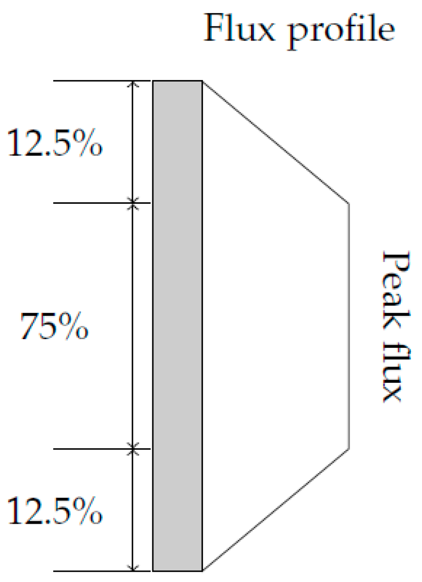
Many aiming strategies have been developed, tested and implemented [3]. Among them, Abengoa Solar considers five vertical points for each of the 24 panels of tubes in order to reach an even flux profile on the central 75% of each panel [4], as shown in Figure 1.
Reduction in spillage loss and improvement of the method were then achieved by SENER at Gemasolar by selecting heliostats with high focal for the central aiming points and heliostats with low focal for the top and bottom points [5]. This method is called deviation-based multi-aiming.
Another approach was investigated by Garcia-Martin et al. and relies on a closed loop automated system [6]. The objective was to optimize the temperature distribution within the volumetric receiver by applying a heuristic knowledge-based heliostat control strategy. Salomé et al. [7] developed an open loop control process based on the Tabu meta-heuristic algorithm and the HFLCAL (Heliostat Field Layout CALculation) approximation model for flux distribution estimations [8]. Besarati et al. developed a similar method but with a genetic algorithm as an optimization method [9]. The ant colony optimization [10] associated with the ray-tracing software STRAL [11] was chosen for the Jülich solar tower tests. The objective is to maximize the receiver output instead of the efficiency. The heliostat field management of the Ivanpah solar thermal power plant relies on the Solar Field INtegrated Control System (SFINCS) developed by BrightSource. The optimization of the heliostats aiming points is achieved by a closed-loop control system that aims to maximize the solar energy input in the receiver while respecting the flux limitations, which are 150 kW/m2, 600 kW/m2 and 300 kW/m2 for the reheater, evaporator and superheater, respectively. Finally, several methods have been described for circular receiver and are summarized by Collado [12].
Most of the aiming strategies were developed for commercial plants and for circular or flat receivers, and the amount of published literature is limited.
The objective of this paper is to assess the performance of an aiming point strategy on an experimental, hence smaller, solar receiver. Due to the complex geometry of the particle-based CSP prototype receiver (a tubular receiver with refractory panels around, see the next section), the APS has to be carried out following two steps. First, an APS at the tubes mid-plane and, second, the integration of the results in a ray-tracing software to account for the tubular geometry of the solar receiver and for the cavity impact. The CSP prototype receiver is presented in the next section. Then, the methodology is detailed. Finally, the consequences of APS on the wall/particles temperature and thermal/optical performance of the receiver are quantified and discussed at steady state and during start-up.
In this paper, the terms “flux” and “flux density” refer to the irradiance, corresponding to the power per surface unit (W/m2).
2. The Fluidized Particle-CSP Prototype
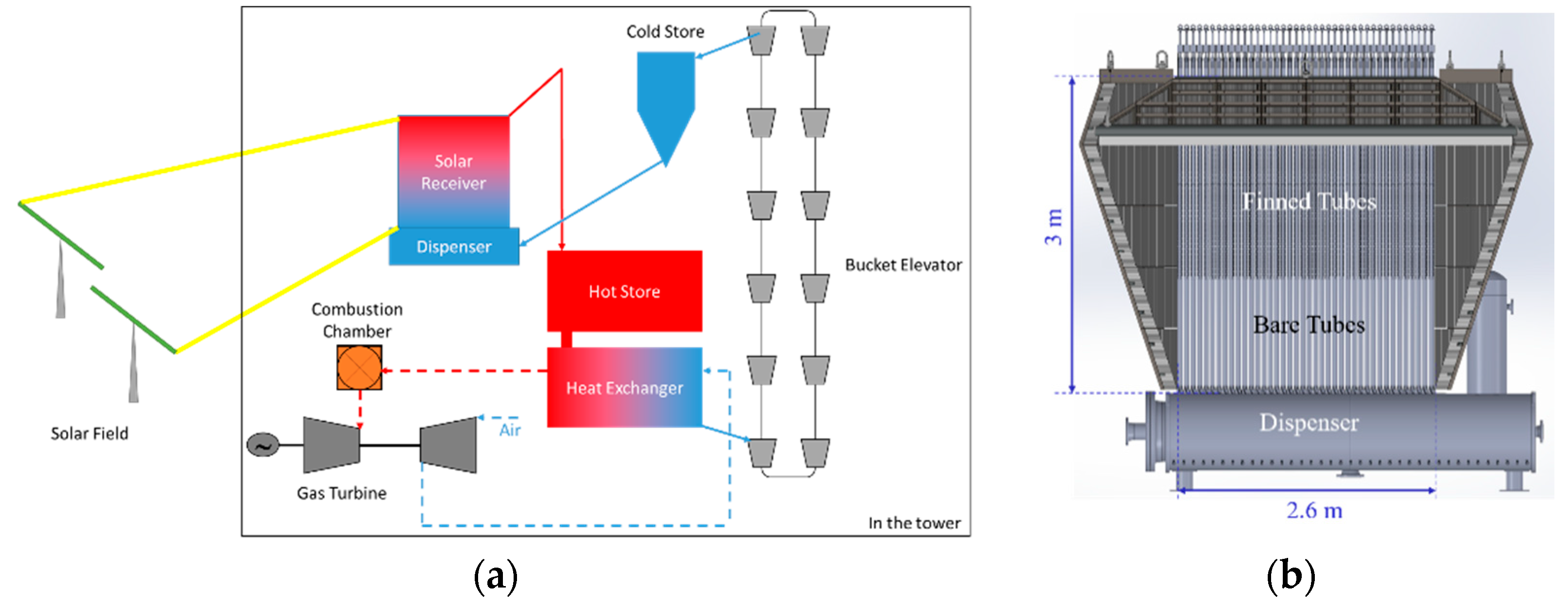
The Next-CSP project (http://next-csp.eu/, accessed on 30 March 2020) aims at demonstrating at prototype scale a complete concentrated solar energy conversion system using high temperature particles as heat transfer fluid and storage medium. It includes a multi-MW fluidized particle-in-tube solar receiver. As shown in Figure 2a, the fluidized particles flow upward from the dispenser in the forty 3 m-long-vertical tubes (Figure 2b) before filling a hot storage tank. A multi-stage fluidized bed heat exchanger and a gas turbine (hybrid or solar-only) constitute the power block. After passing through the heat exchanger, the cooled particles are collected in the cold store before flowing back to the solar receiver. Pressurized air of the gas turbine compressor is preheated by the hot particles in the fluidized bed heat exchanger before reaching the combustion chamber that overheats air up to the turbine inlet temperature (hybrid mode operation). The nominal conditions are a pressure of 6.5 bar, a turbine inlet temperature of 1000 °C, a gas flowrate of 8 kg/s and an electrical power of 2 MWel.
The concept of the fluidized particle-in-tube solar receiver was proven at 150 kW scale in the framework of the CSP2 project [13].
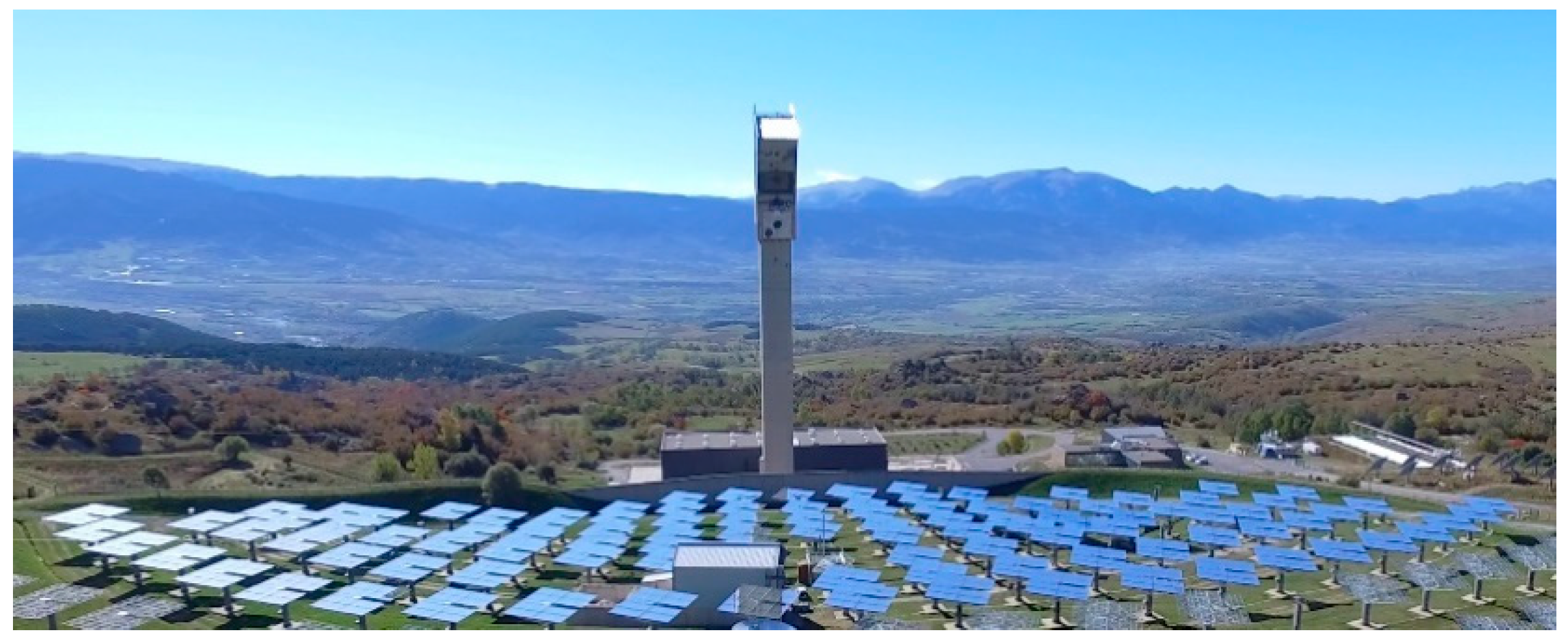
The Next-CSP system is tested at the Themis site in Targasonne (France). The Themis solar tower consists of a 104-m high tower and a field of 107 heliostats each with a 54 m2 reflective surface, as shown in Figure 3. The Next-CSP system is installed between the third and the fourth floor of the tower, corresponding to 83 m and 92 m in height.
As abovementioned, the Next-CSP absorber of the solar receiver consists of 40 vertical tubes in which the fluidized particles flow upwards. The particles are Olivine (magnesium silicate) with a mean diameter (d50) of 80 μm. Their density and specific heat are 3300 kg/m3 and 1.15 kJ/kg.K, respectively [14]. Each tube is made of two sections: 1 m of bare tube (lower part) and 2 m of finned tube. The tubes are 50.8 mm in outer diameter and there is a 14.2-mm gap between each tube. As shown in Figure 2b, a refractory panel is located behind the tubes to reflect the concentrated light passing through the gaps between the tubes onto the back of the tubes. In addition, a half cavity made of refractory panel is positioned around the absorber to form the receiver and improve the thermal efficiency. The angles of the cavity panels result from the position of the most Eastern, Western and Northern heliostats of the already existing solar field. This situation leads to a non-optimal heliostat layout with respect to the solar receiver and a high value of spillage when the aiming point strategy is applied. Nevertheless, this constraint does not affect the methodology developed hereafter.
3. Methodology
APS is essential to uniformly heating up the particles in all the 40 tubes in addition to the operation constraint of the solar receiver cited previously.
APS is investigated by applying the Tabu search [7], a meta-heuristic method, associated with the convolution–projection optical model UNIZAR (Universidad de Zaragoza) [15]. The Tabu search is an iterative method based on the hill climbing algorithm. At each iteration, a random aiming point is assigned to a random heliostat. If the cost function is improved, the heliostat is kept at this position, if not, it is sent back to its original aiming point and the aiming point is not re-assigned to this heliostat, hence the name “Tabu” of the method.
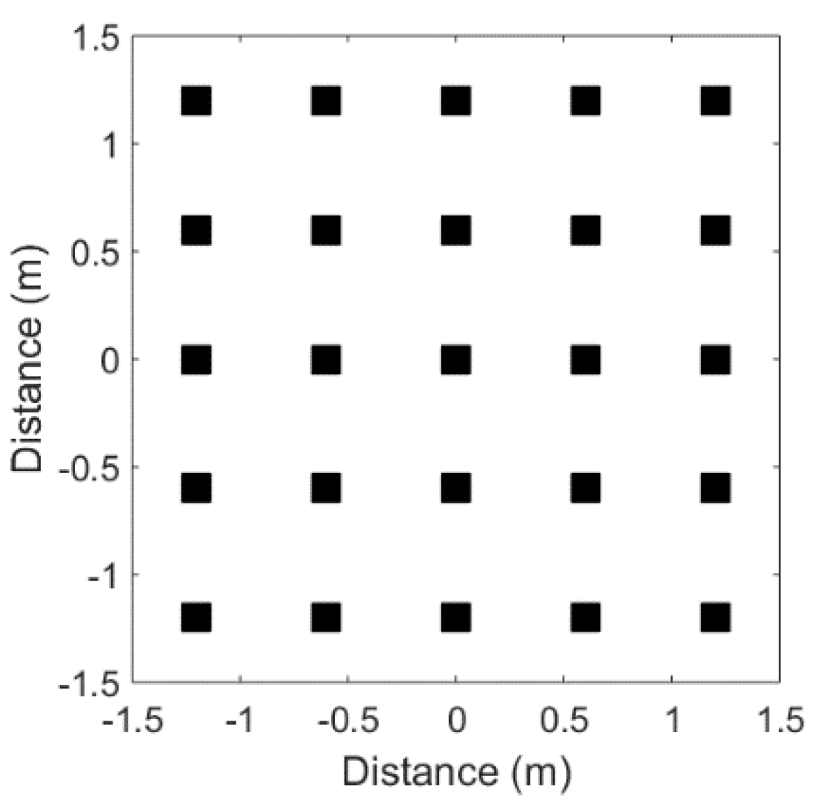
The slope error of the mirror is set to 1.5 mrad, which is a value commonly measured on the Themis heliostats. The APS is carried out on an aperture plane located on the mid-plane of the tubes. A 3 m × 3 m aperture plane is considered and 25 points are defined as shown in Figure 4. The choice of 25 points was the result of a trade-off from previous simulations. The distance between the points is 60 cm horizontally and vertically.
Hereafter the parameters of the aiming point strategy are defined.
The cost function is the root-mean-square deviation between an objective normalized flux distribution and the normalized simulated flux distribution.
The spillage loss (SL) is defined as:
where QAPS and QNoAPS are the power intercepted by the 3 m × 3 m aperture with and without APS (single aiming point for the entire heliostat field), respectively.
With APS, the spillage loss must be monitored and kept below a certain threshold. In our case, the spillage loss is limited to a maximum of 30% in the Tabu search (it is not the achieved value but the maximum value).
The objective normalized flux distribution is defined as a typical Gaussian distribution horizontally and the following normalized surge function vertically:
where xpeak is the vertical location of the maximum flux density and b is a parameter that allows modification of the shape of the vertical distribution (flat or sharp). Although previous studies showed that the mean flux density on the receiver must not exceed 500 kW/m2 to avoid hot spots [16], the limiting factor in this study is the maximal wall temperature given by the thermal model (presented below). Consequently, the maximum flux density can be slightly higher than 500 kW/m2 in tube section where the temperature difference between the wall and the particles is at its maximum.
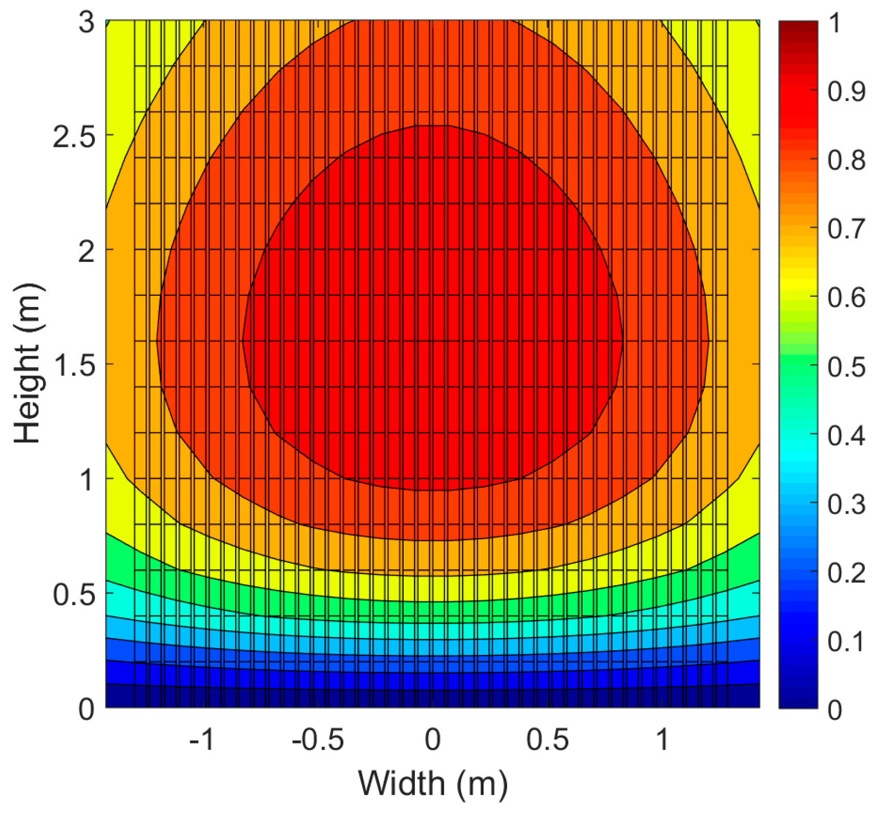
Figure 5 shows a typical objective normalized flux distribution with a schematic view of the tubes’ location. For the reference case, the maximum flux is located at the middle height of the tube (xpeak = 1.5 m), and the standard deviation of the Gaussian distribution σ2 and the parameter b are set to 12 and 0.5, respectively.
Daily APS (a single aiming point for each heliostat throughout the day) is examined and compared to hourly APS (aiming points changing every hour) to easily control the heliostat field during a full day of operation.
Results of APS are introduced into SOLTICE (SOLar Simulation Tool in ConcEntrating optics), a new open-source ray-tracing software developed by the CNRS-PROMES (Processes, Materials and Solar Energy) laboratory and Meso-Star SAS (simplified joint-stock company) [17]. SOLTICE is an upgrade of the previous version Solfast with reduced computation time. It is based on the same algorithm as Solfast which was validated in previous studies [18] and provides more options in terms of geometry and reflection behavior of surfaces. SOLTICE uses the Yet Another Markup Language (YAML) language to create geometries. It is designed to efficiently handle complex solar facilities. Indeed, the CAD model can be imported and therefore a complex ray’s path can be simulated. The influence of the variation of surface optical properties with wavelength can also be taken into account.
The flux distribution on each tube computed by SOLTICE is post-processed and considered in a simplified thermal model developed with the Matlab® software [19]. The thermal model is based on the Net Radiation Method, which establishes the balance on heat flux and radiosity.
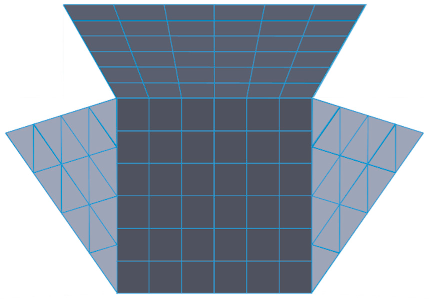
The discretization of the tubes for the thermal model is performed by dividing each of them into 15 parts in height, and considering the front and the back of the tube. This discretization results in 1200 elements for the forty tubes (30 elements per tube). The cavity is discretized in 104 elements, as shown in Figure 6 when the cavity is unfolded.
The flux density coming from SOLTICE is assigned to each element and a net power absorbed per element is defined as follows:
with Ai as the element area (m2), the solar incident flux density after the radiative balance in the solar spectrum (0.3 μm ≤ λ < 3 μm) achieved in SOLTICE (W/m2), Fij the view factor from element i to element j (-) and the radiosity of element i in the infrared spectrum (λ ≥ 3 μm) (W/m2).
The overall heat transfer is calculated based on experiments on a single bare tube [20] and finned tube [21] at the 1-MW solar furnace of CNRS-PROMES (Odeillo, France). The reference values of the wall-to-fluidized bed heat transfer coefficient htr,ref in the previously cited papers are calculated with the logarithmic mean temperature difference ΔTlm [22] using the internal wall temperature as follows:
with as the surface heat transfer (W/m2) and
with as the internal wall temperature (inlet/outlet) (K) and Tp,i/o the particle temperature (inlet/outlet) (K).
However, due to the structure of the thermal model, the surface heat transfer is calculated between the front wall and the particles by the equation:
with htr as the overall heat transfer coefficient (W/m2.K), Tfront the front wall temperature (K) and Tpart,mean the mean particle temperature between the inlet and the outlet (K).
Therefore, other values of overall heat transfer coefficient than the abovementioned experimental results are used to fit the thermal model architecture. These values were calculated by applying the structure of the thermal model to the experimental results on a single tube (bare and finned). The overall heat transfer coefficient was fitted in order to reach the experimental absorbed power in the particles. The calculated values for the bare and finned tubes are 350 W/m2.K (instead of the reference value of ~800 W/m2.K [20]) and 500 W/m2.K (instead of the reference value of ~1200 W/m2.K [21]), respectively.
The tubes should have been made in Inconel but, due to cost issues, a lower grade of alloy (Stainless Steel) painted with Pyromark 2500 was used. Nevertheless, the maximum wall temperature allowed in this study is 1000 °C, corresponding to the limit given by Inconel. The optical properties of the Pyromark 2500 [23] and of the diffuse refractory panels (ALSIFLEX®) [24] used for the cavity are shown in Table 1.
In the following sections, three indicators are defined. First, the optical efficiency ηopt and thermal efficiency ηth are defined as follows:
with as Qaperture the power reaching the receiver aperture (W), I the direct normal irradiation (W/m2) and Amirror the mirror surface of the heliostat field (m2).
with Qparticles as the power absorbed by the particles (W).
Finally, a temperature deviation (TD) is calculated as follows to evaluate the uniformity of the particle outlet temperature in each tube,
with n as the number of tubes (-), Ti the outlet particle temperature of tube i (K) and the mean particle outlet temperature (K).
4. Results
The performance of the solar receiver depends considerably on the APS. This section summarizes the simulation results. First, the performances of the receiver without APS are presented and compared with the case with APS. Then, the influence of the spillage loss threshold on the APS results is investigated as well as the influence of aiming point attribution for each heliostat. Daily and hourly APS are investigated and confronted. The following three subsections give an overview of the receiver thermal performance depending on the objective normalized flux distribution applied to the APS. Finally, the method to increase the power on the receiver during start-up is detailed. All the simulations are carried out March 21 at solar noon, with a DNI (Direct Normal Irradiance) of 950 W/m2. The particles enter at 400 °C and the total mass flowrate is 5 kg/s.
4.1. Performance without APS
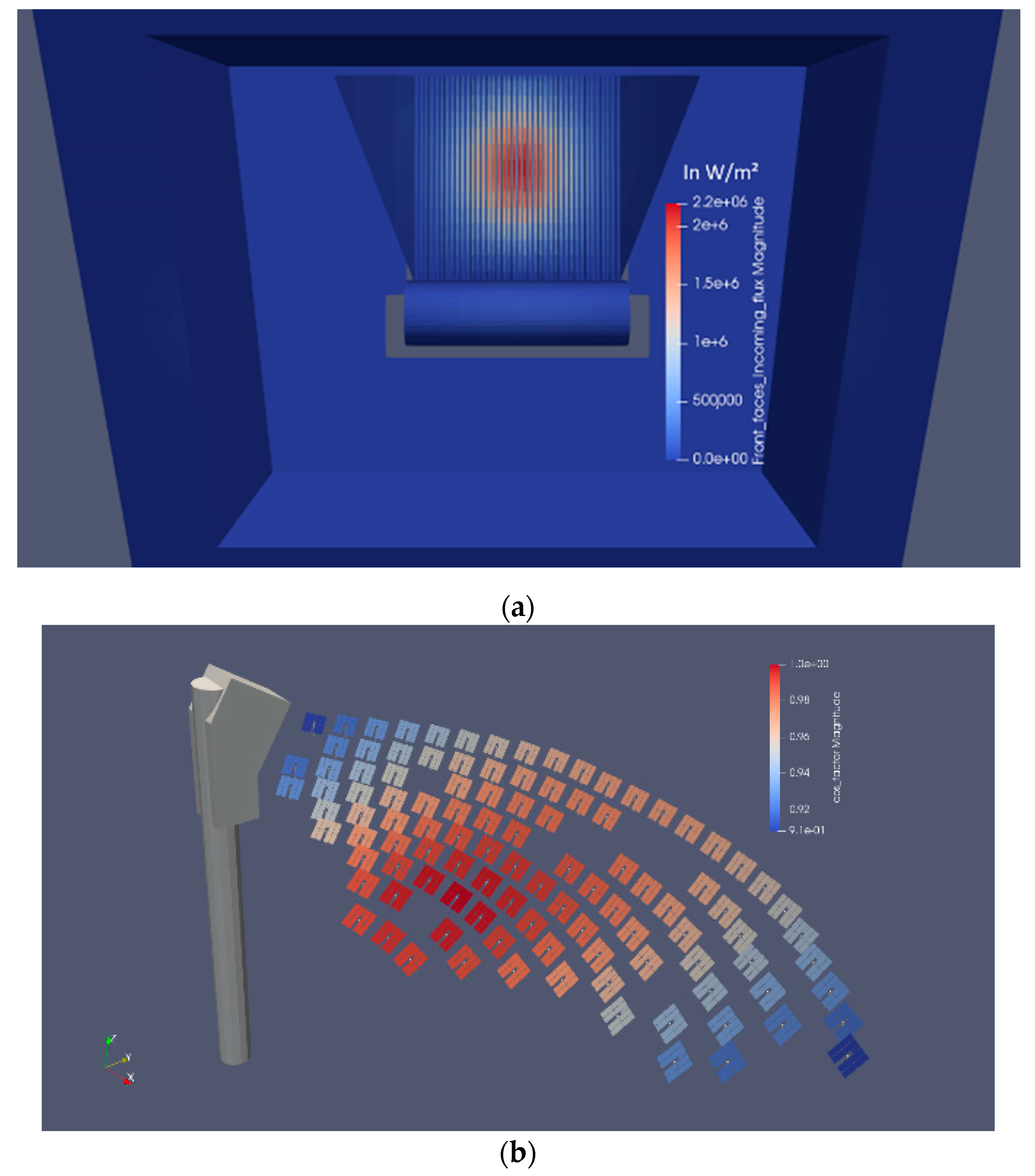
Figure 7 shows the simulation results of SOLTICE software observed in Paraview when no APS is applied. The maximum flux density on the tubes is 2.2 MW/m2 and the corresponding total absorbed power is 3.9 MW.
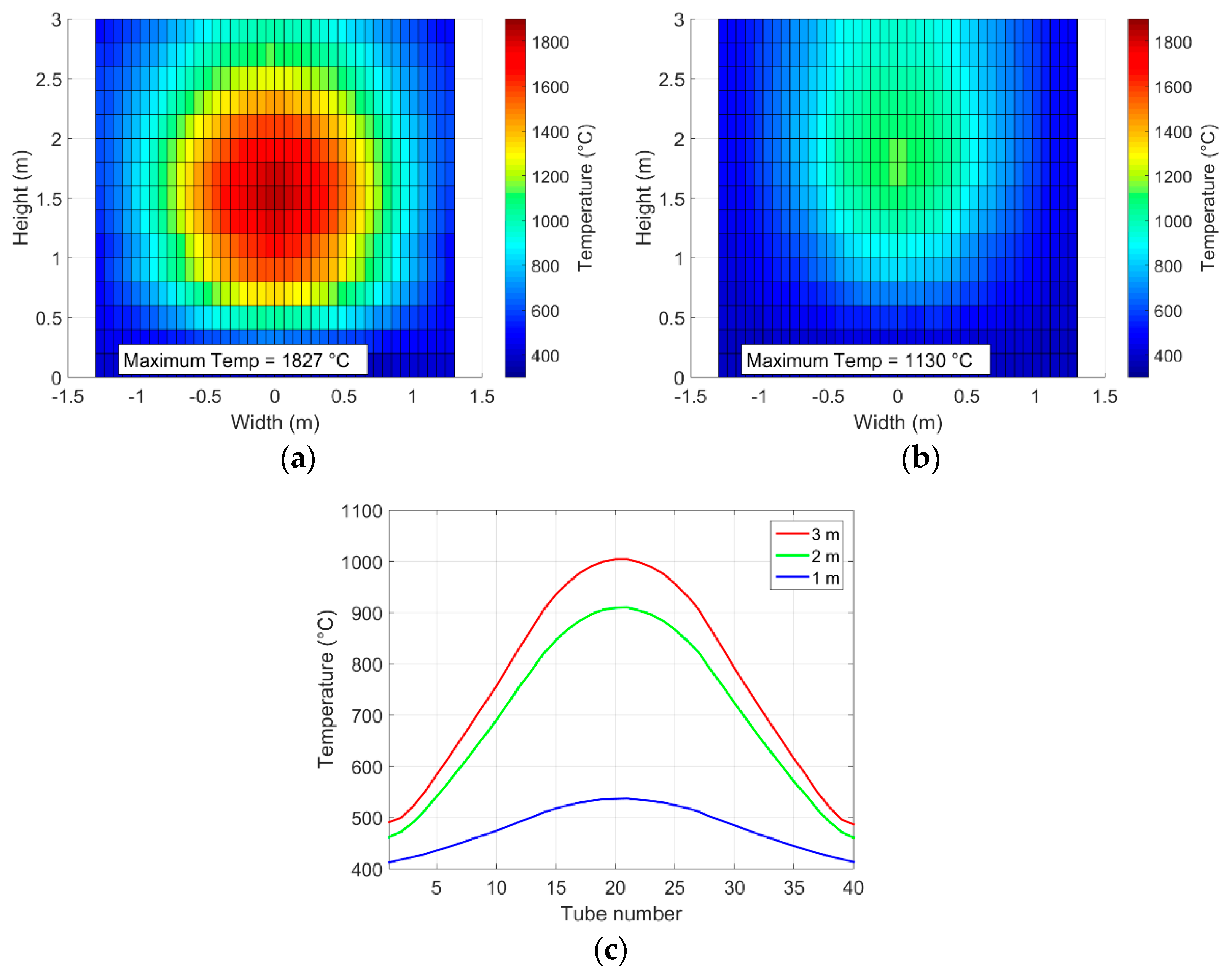
Despite a high optical efficiency in this case (80.8%), the results are not acceptable for operating the receiver. Figure 8 shows that the maximum tubes temperature (1827 °C) is much higher than the melting point of SS 310S, due to a maximum flux density of 2.2 MW/m2. Furthermore, the particle temperature in the 40 tubes is very heterogeneous, with a much higher particle temperature in the middle tubes.
These results prove the need to apply an APS in order to preserve the solar receiver, extend its lifetime and obtain more uniform particle temperature in all the 40 tubes.
4.2. Performance with the Reference Case APS
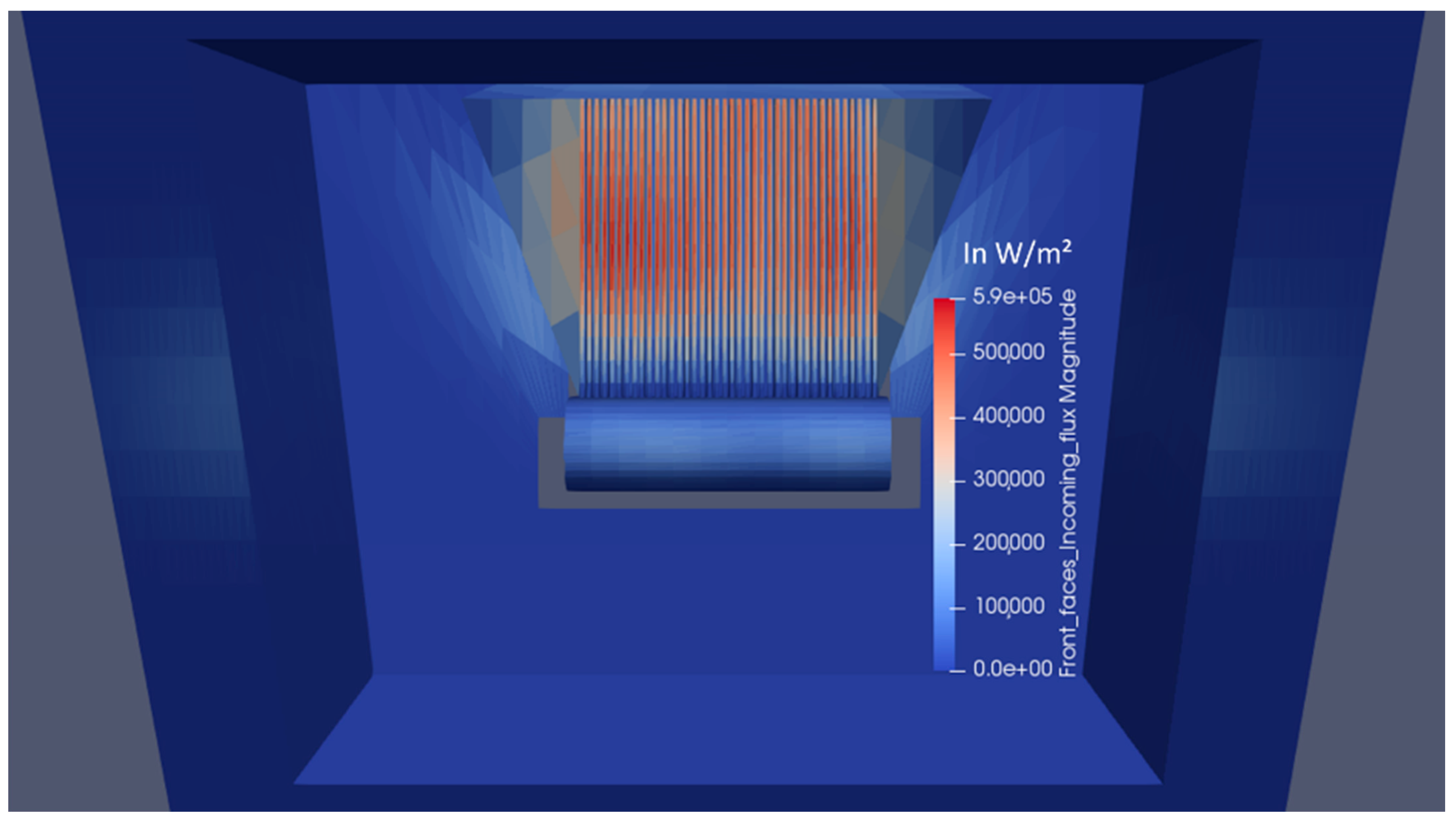
By applying the reference case APS, the maximum flux density drops from 2.2 MW/m2 down to 590 kW/m2, as shown in Figure 9 which is displayed in Paraview. This visualization allows observation of the spillage on the tower cladding.
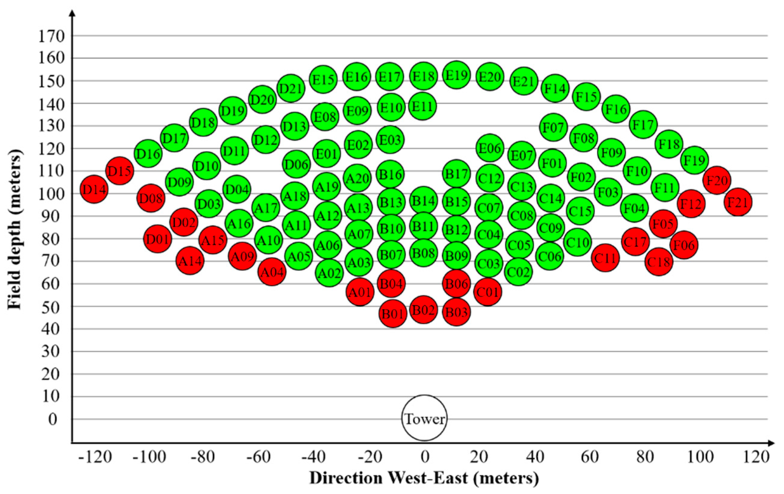
Despite the decrease in the maximum flux density, the maximum tube temperature is 1055 °C, hence still above the accepted limit. Therefore, 24 heliostats are removed from the simulations, as shown in red in Figure 10. The selected heliostats are the most western/eastern and the closest to the tower.
With this layout, the maximum flux density drops down to 460 kW/m2 and the maximum wall temperature decreases down to 976 °C. Removing these 24 heliostats allows an increase in the optical efficiency from 69.7% up to 73.7%, and the thermal efficiencies from 47.1% up to 50.9%.
In the following sections, only the 83 heliostats in green in Figure 10 are considered.
4.3. Influence of Spillage Loss Threshold on the APS Performance
The influence of the spillage loss threshold (from 15% to 30%) on the APS performance is analyzed in this section. Table 2 shows the evolution of the cost function and the spillage loss for the four cases.
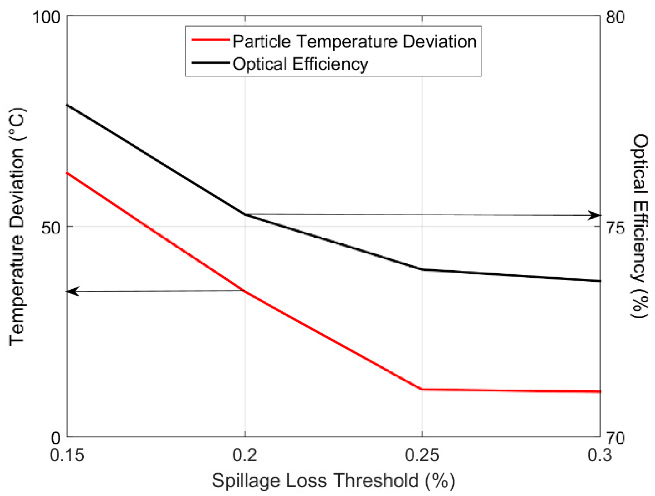
The spillage loss threshold has a strong influence on the APS performance. Indeed, by allowing 30% of spillage loss threshold, the cost function is around 0.05 compared to 0.22 for 15% of spillage loss threshold. The resulting maximum flux density is 650 kW/m2 for the 15% threshold, corresponding to a maximum tube temperature of 1233 °C. By increasing the spillage loss threshold, the optical efficiency inherently drops but the particle temperature becomes uniform at the exit of the 40 tubes. When allowing 30% of spillage, the threshold of 30% is not reached because there is no more possibility to improve the cost function. Figure 11 shows the evolution of the optical efficiency and of the temperature deviation as a function of the spillage loss threshold.
The spillage loss threshold is maintained at 30% in the following sections to focus on the influence of the other APS parameters.
4.4. Heliostat Aiming Points Attribution
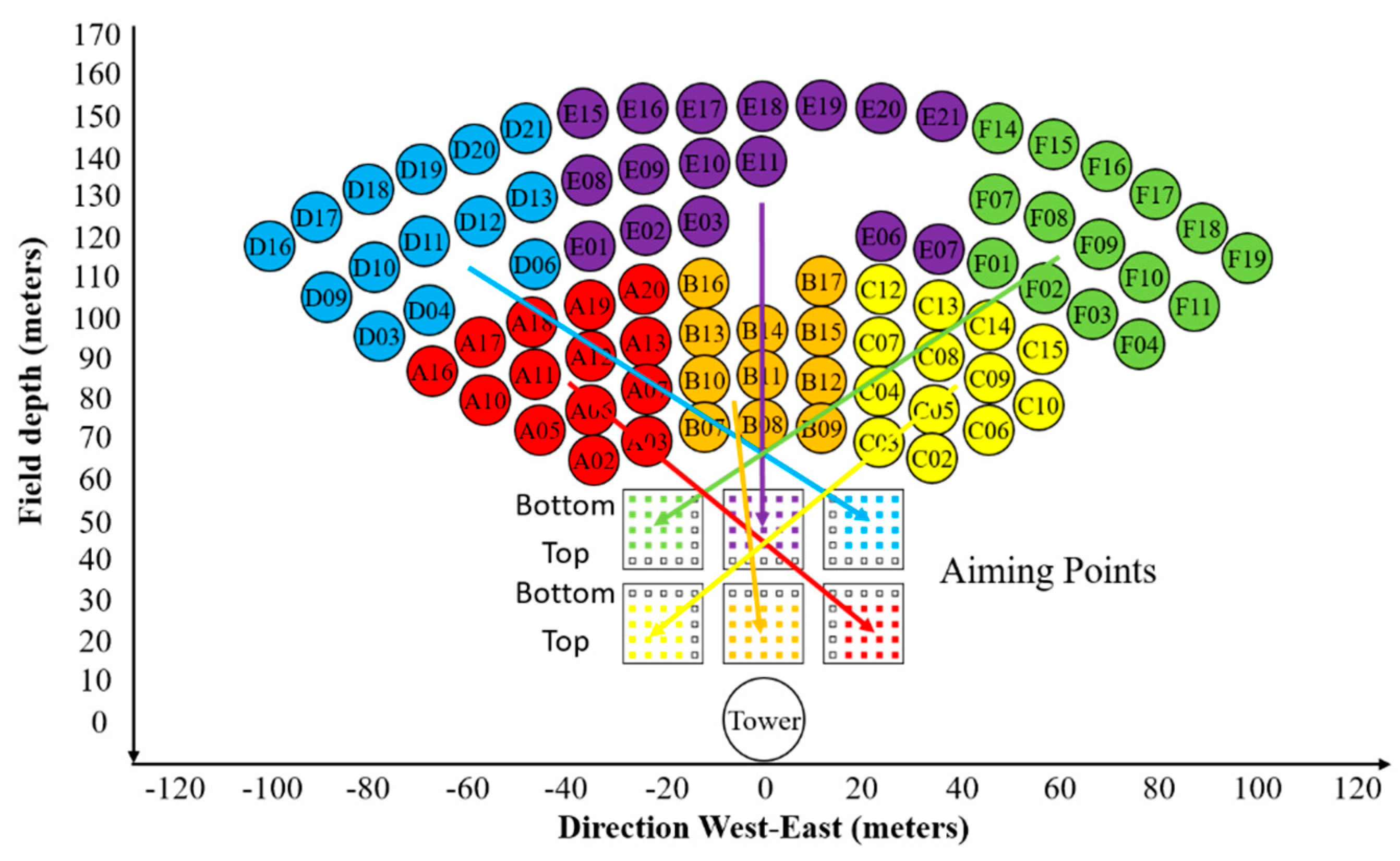
In all the previous simulations, each group of heliostats, depending on their location in the field (A to F group of heliostats), had an attribution of aiming points for the APS in order to minimize as much as possible the spillage due to the tower cladding. Indeed, the Next-CSP receiver is located in the tower and the cladding tilted shape (cf. Figure 7b) is not adapted to the absorber vertical design. The absorber’s tubes must be maintained vertical to respect a homogeneous fluidization of the particles. The attribution of aiming points is shown in Figure 12.
If this strategy is not applied, therefore if each heliostat can aim at the 25 aiming points, it can be observed in Table 3 that the cost function is slightly lower and the spillage loss threshold is reached.
The main consequence resulting from the ray-tracing simulation is a drop in the optical efficiency from 73.7% down to 65.1%, mostly due to an increase in spillage on the cladding and around the solar receiver. Therefore, the attribution of aiming points for each group of heliostats is maintained in the following sections.
4.5. Hourly vs. Daily APS
Daily APS is investigated and compared to hourly APS (previously considered) in order to facilitate the control of the heliostat field during a complete day. The DNI varies between 600 W/m2 and 950 W/m2 during the day. For the daily APS, the cost function considers the simulated and objective normalized flux distributions from 8 a.m. to 4 p.m. every hour. Table 4 shows the evolution of the cost function and the spillage loss as a function of the iteration number for hourly (8am, 10am and noon) and a daily APS.
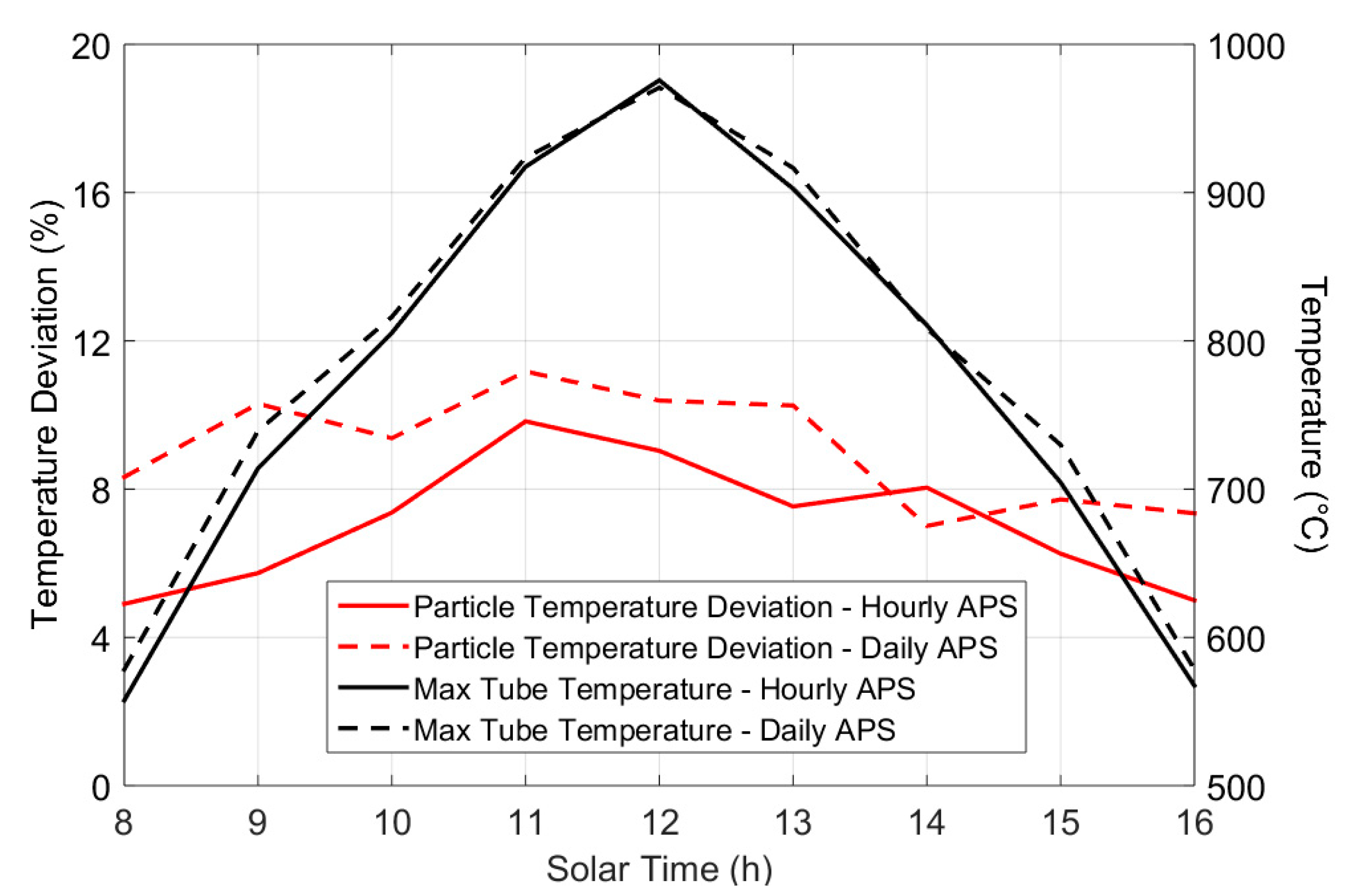
The convergence of the Tabu search for both APS is reached after ~2000 iterations. Similar values of the spillage losses and the cost function are found for all strategies. This behavior is confirmed by comparing the particle temperature deviation and the maximum tube temperature that are obtained with hourly and daily APS (Figure 13). In Figure 13, the particle flowrate is maintained constant during the day, which will not be the case in real operation.
This analysis confirmed that a daily APS is an interesting option to control the heliostat field. Given the low power for high sun incident angle (morning and afternoon), the daily APS should be achieved with the whole solar field (107 heliostats) and lower particle flowrate, and some heliostats should be defocused and refocused before and after noon, respectively.
4.6. Influence of Horizontal Flux Distribution Profile on Particle Temperature
The objective normalized flux distribution is modified horizontally (normal distribution with different standard deviations) to determine its influence on the particle outlet temperature uniformity. The effect of the diffuse reflective cavity can be observed in Figure 14. Indeed, the particle temperature in the side tubes (1 and 40) is higher than in the neighboring tubes (2 and 39) due to the reflection of the concentrated solar radiation on the side cavity refractory panels.
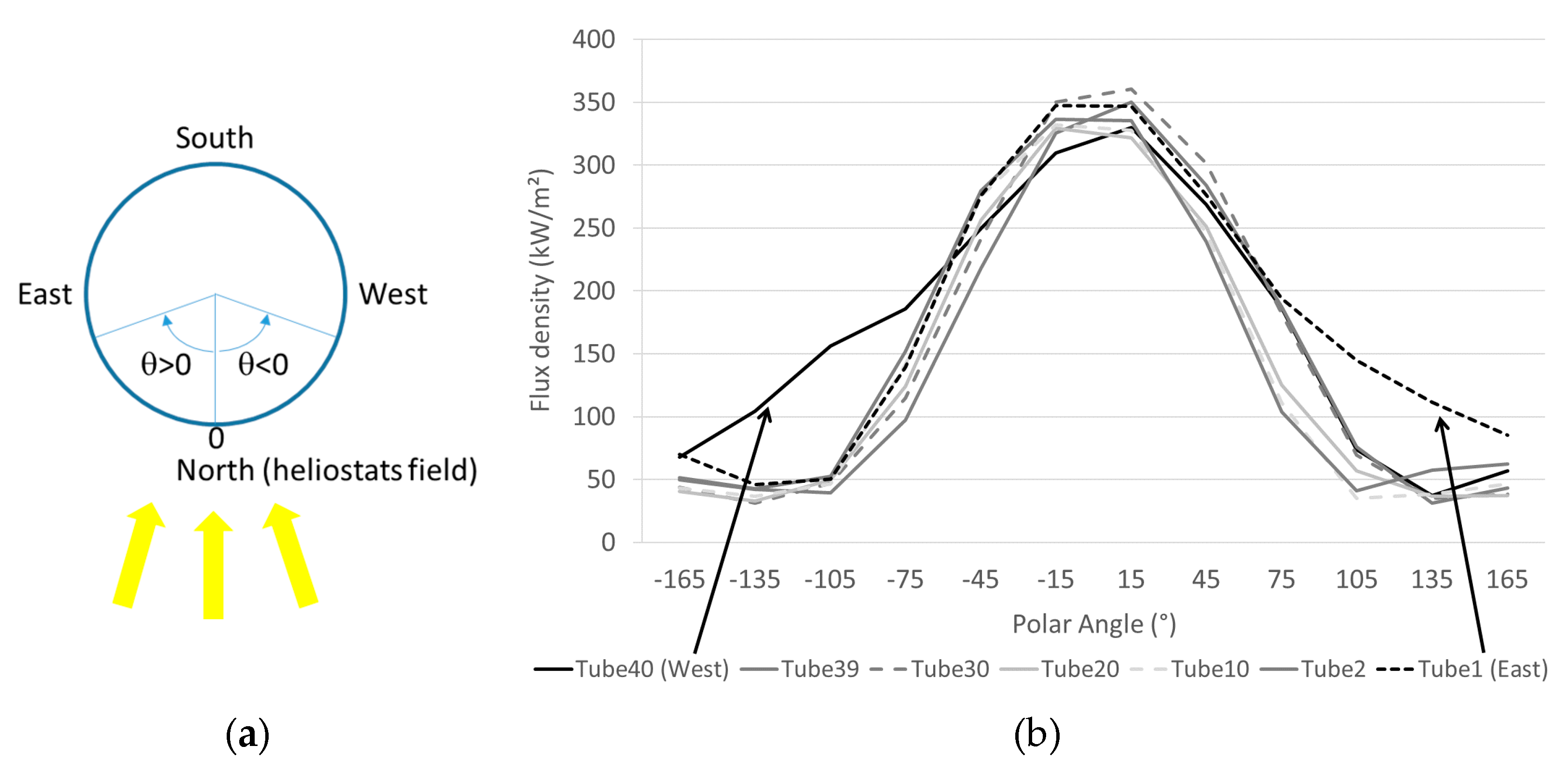
This trend is confirmed in Figure 15b that illustrates the effect of the solar radiation diffusion on the cavity lateral panels on the side tubes’ radial flux density profile for the reference case.
For each tube, the radial distribution is strongly asymmetrical relative to the north/south plane, as the back of the tubes is only enlightened by the solar beam reflection on the diffuse back refractory panel while the front of the tubes receives the direct concentrated solar radiation. However, the radial distribution is rather symmetrical relative to the east/west plane as shown in Figure 15a. Figure 16 confirms this trend. It shows the solar flux density as a function of the tube height (middle tube number 20) for different polar angle.
The low flux density at the bottom of the tube is due to the incident solar flux blocked by the dispenser.
Table 5 specifies the particle temperature deviation as well as the maximum tube temperature for each case. The case with a horizontal standard deviation σ2 = 12 results in the most uniform particle outlet temperature and the lowest maximum tube temperature.
For these three cases, the mean particle outlet temperatures are, respectively 673 °C, 668 °C and 664 °C.
4.7. Influence of Vertical Flux Distribution Profile on Thermal Performance
In this section, the objective normalized vertical flux distribution is modified, flattening it more or less by varying the parameter b in the normalized surge function. Figure 17 shows the influence of the flattening (b = 0.1) and the sharpening (b = 1.5) of the vertical flux distribution on the tube temperature profile. Sharpening the vertical flux distribution leads to higher maximum tube temperature due to higher flux density.
The optical efficiency increases from 65.7% up to 76.6% when the vertical distribution is sharpened. With a rather similar thermal efficiency of the receiver of approximately 50%, sharpening the vertical flux distribution allows increase in the particle temperature from 647 °C to 680 °C, but is limited by the maximum tube temperature that must not exceed 1000 °C.
In addition, the transition from bare tubes to finned tubes at 1-m height is represented by a thicker horizontal lines, and results in a discontinuity of the tube temperature due to the better heat transfer between the tube and the particles above 1 m.
4.8. Influence of Peak Flux Location on Thermal Performance
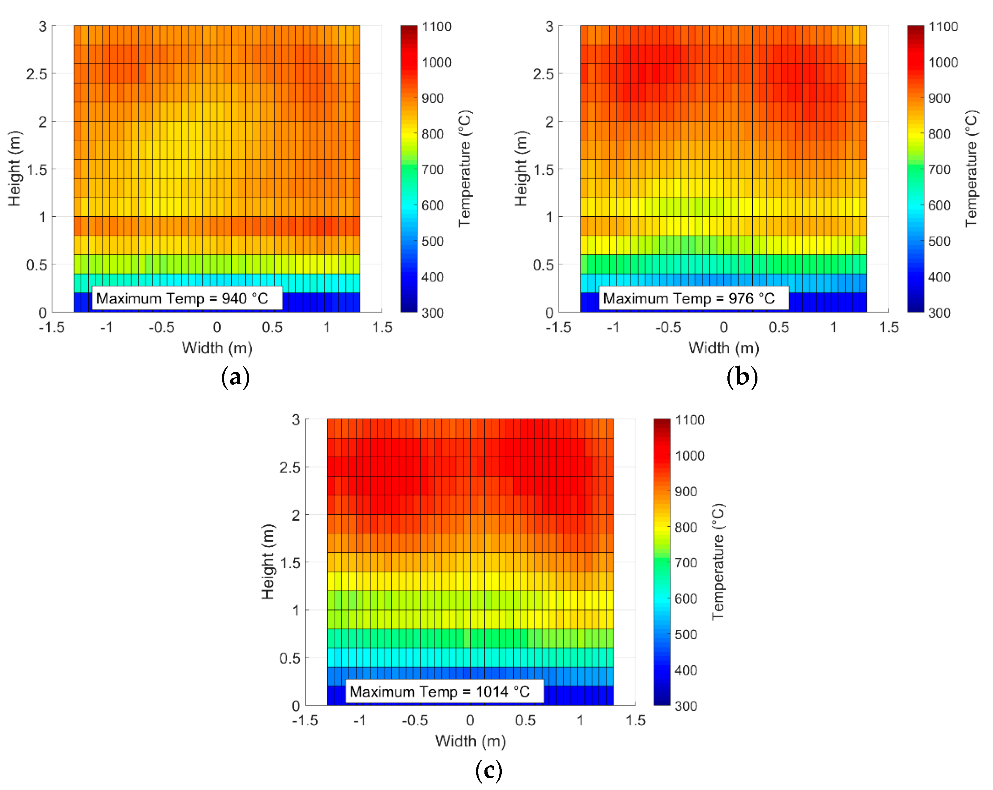
The location of the peak flux is modified from 1.2 m to 1.8 m on the objective normalized flux distribution in order to calculate the corresponding optical/thermal performance and the wall temperature. Figure 18 shows that the maximum tube temperature increases from 940 °C up to 1014 °C when the peak flux location moves from 1.2 m to 1.8 m, respectively.
The maximum optical and thermal efficiencies are obtained for the last case (1.8 m), leading to the highest particle outlet temperature of 673 °C, but the maximum tube temperature exceeds the limit of 1000 °C. Therefore, the location of the peak flux must respect a tradeoff between the maximum tube temperature and the particle outlet temperature.
4.9. Summary of the Performance Analysis
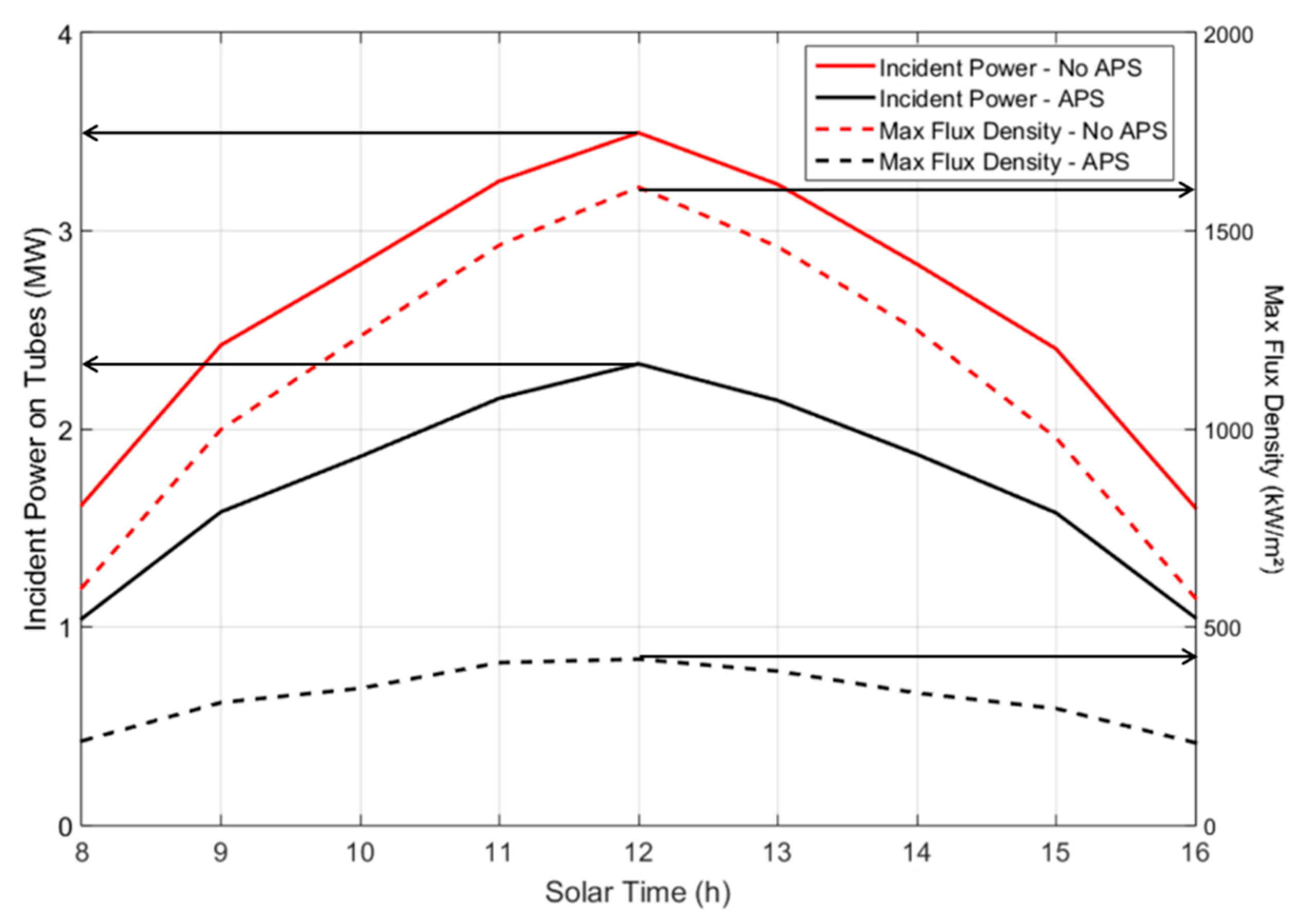
Aiming point strategy leads to a considerable decrease in the highest flux density on the receiver tubes, hence on the maximum temperature on the receiver tubes. The thermal gradient on the tubes is also reduced. Figure 19 shows that reducing the maximum flux density at noon from 1.6 MW/m2 down to 420 kW/m2 results in a drop in incident power on the tubes from 3.5 MW down to 2.3 MW.
Modifying the horizontal flux profile has an inherent influence on the particle temperature deviation. However, the shape of the vertical flux profile as well as the peak flux location strongly affects the performance of the solar receiver and the maximum tube temperature.
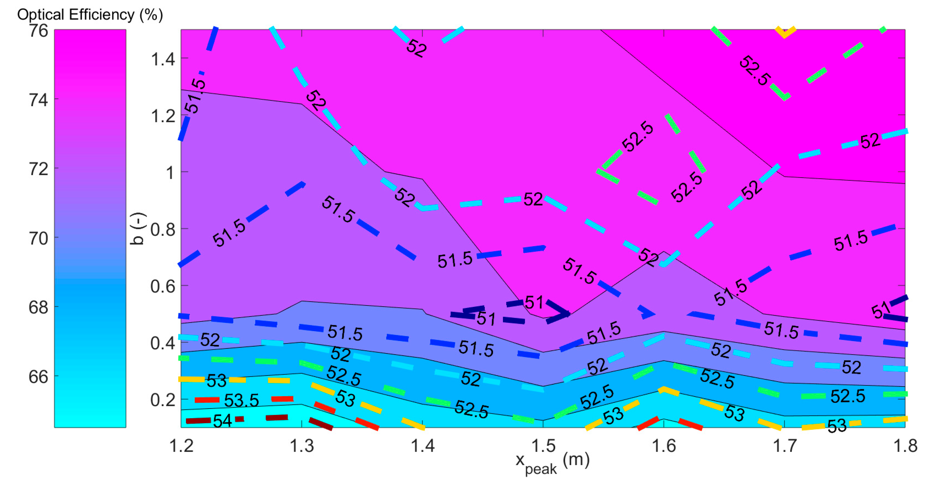
Figure 20 presents the optical and thermal efficiencies for different peak flux locations and vertical flux profiles. The higher thermal performance is observed for lower optical efficiency, and hence lower tube temperature.
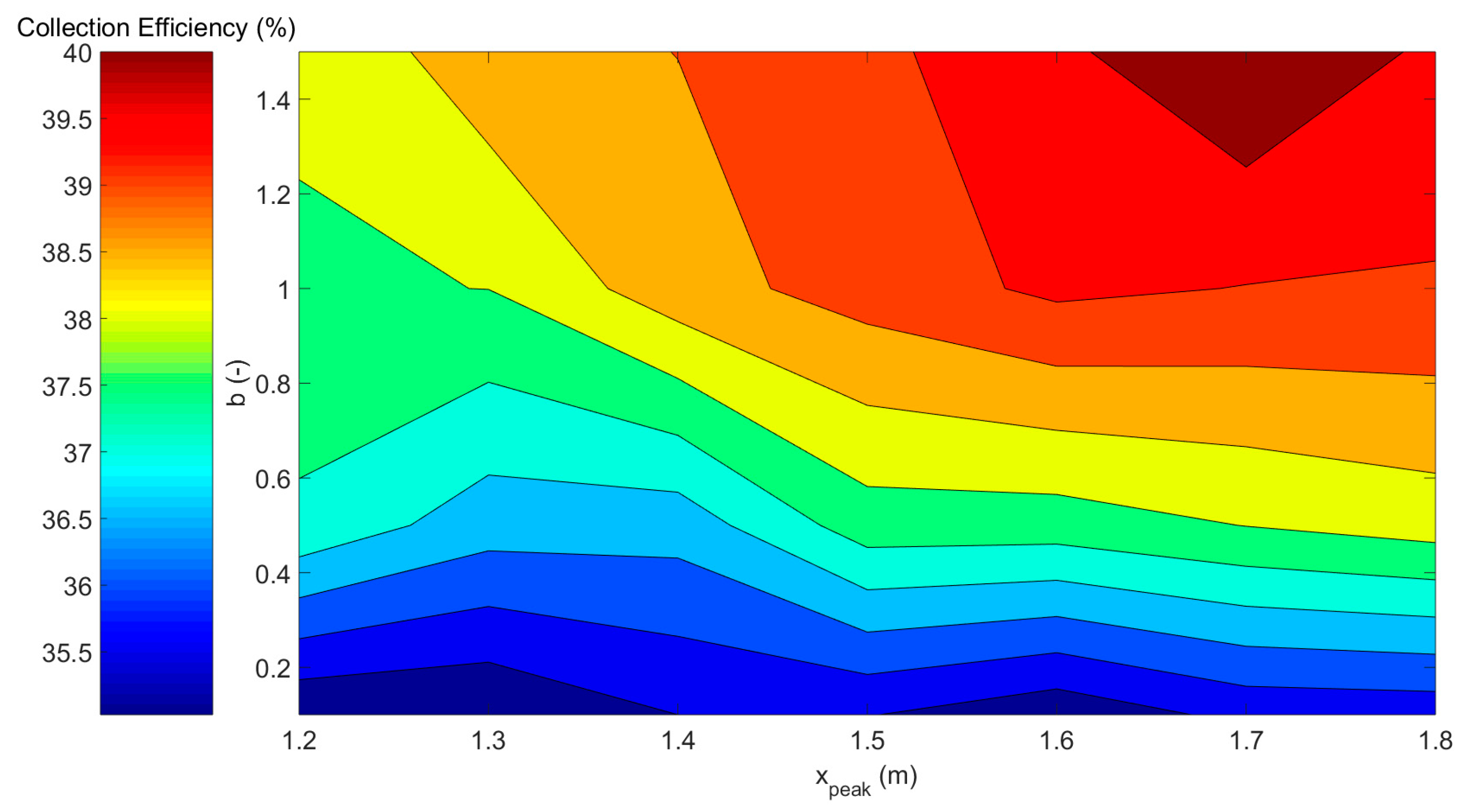
To obtain a better assessment of the system performance, the collection efficiency, corresponding to the product of the optical and thermal efficiency is illustrated in Figure 21.
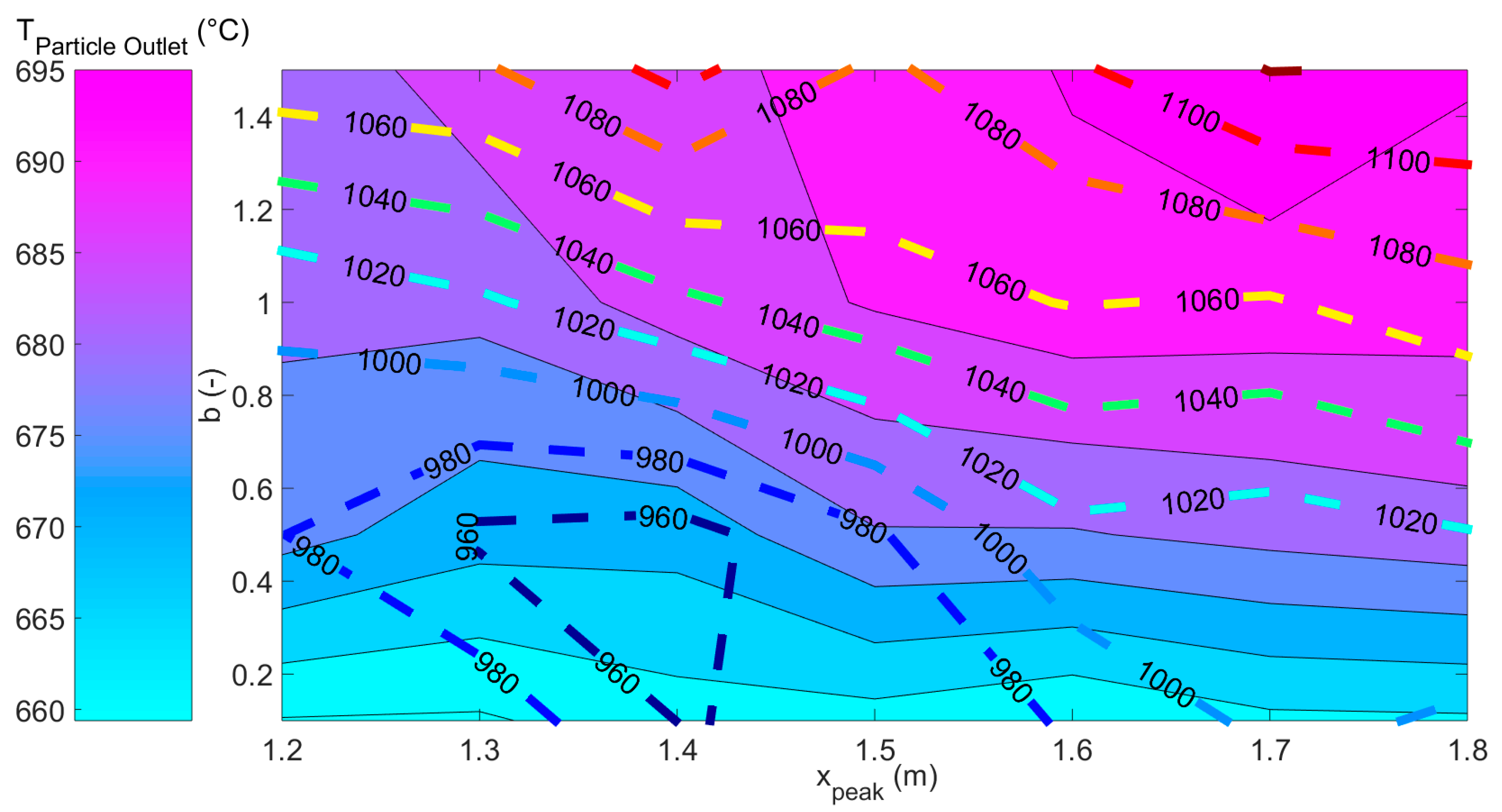
The influence of the peak flux location is rather low when the vertical flux profile is flattened (b ≤ 0.6). However, for a sharp vertical flux profile, higher collection efficiencies are achieved when the peak flux is located at the upper part of the tubes. The particle outlet temperature is directly correlated to the collection efficiency, as shown in Figure 22.
The limitation in maximum tube temperature results in operation conditions corresponding to the bottom left zone (flattened vertical flux distribution and low height of peak flux). The reference case considered in this study corresponds to a point in this zone, and leads to a particle outlet temperature of 680 °C and a maximum tube temperature of 977 °C.
4.10. Power Increase during Start-Up with Aiming Point Strategy
Increasing the power uniformly on the forty receiver tubes is essential to obtain a similar particle outlet temperature in each tube while controlling the tube wall temperature during start-up.
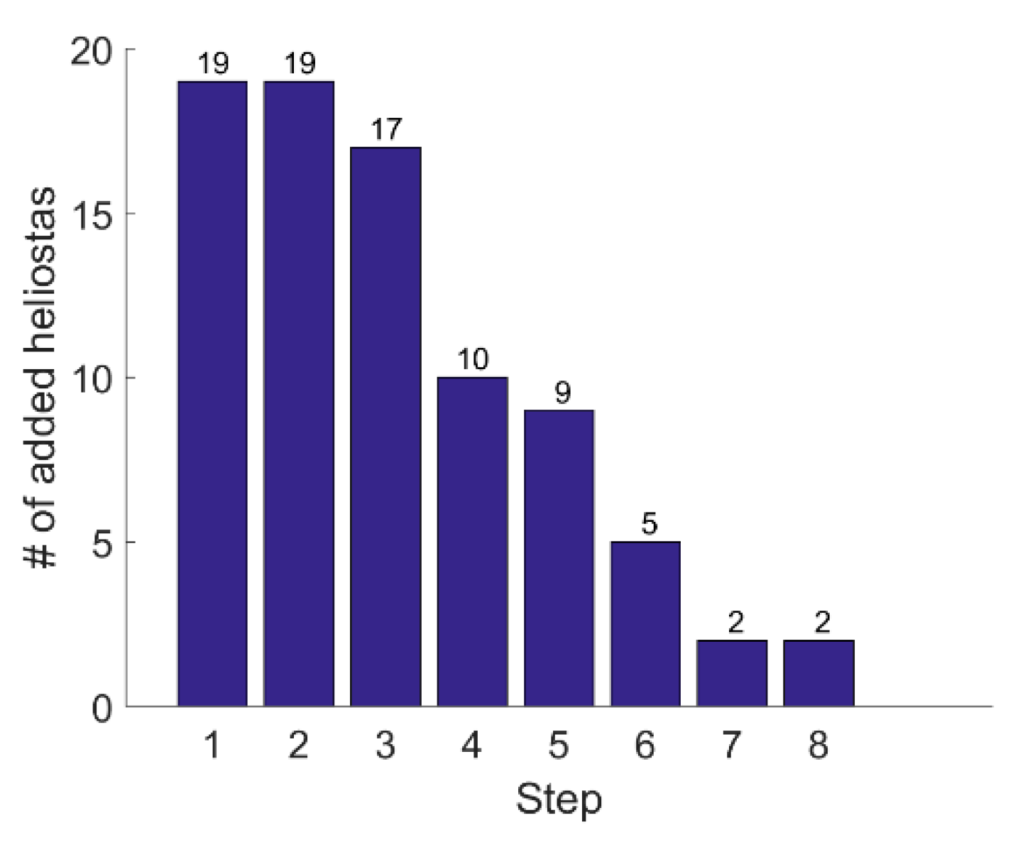
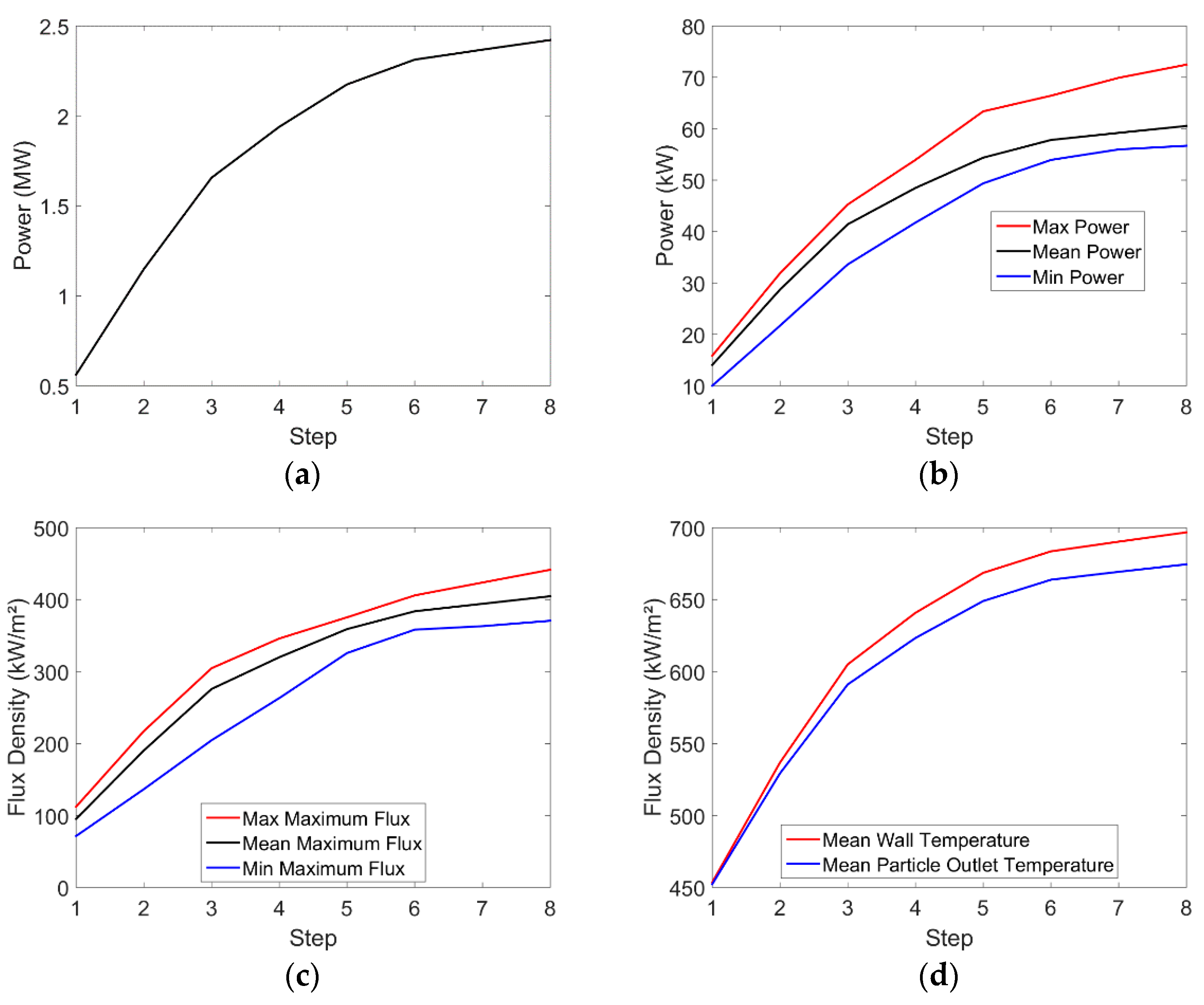
A method was elaborated to select the appropriate heliostats in order to increase the power gradually while keeping similar power and flux densities on the 40 tubes. For each step, one heliostat, if existing, is assigned to each aiming point of the grid. It leads to eight steps with increasing solar power to end up with the 83 heliostats focusing on the solar receiver.
Figure 23 shows the number of heliostats added per step while Figure 24 presents the evolution of the total power, the min/mean/max power, the min/mean/max maximum flux density on the tubes and the mean particle outlet and wall temperature as a function of the step. The particle flowrate is constant during the start-up and the DNI is kept at 950 W/m2.
It confirms that the power increases gradually, with a reasonable power difference on the tubes. The maximum flux density is quite similar for each tube along the steps.
The gradual increase in power needs to account for the sun position while carrying out this operation, the duration required to achieve each step with the heliostats focusing, but also the DNI evolution. However, these results show that the method allows keeping rather uniform power and flux density on each tube during the gradual power increase.
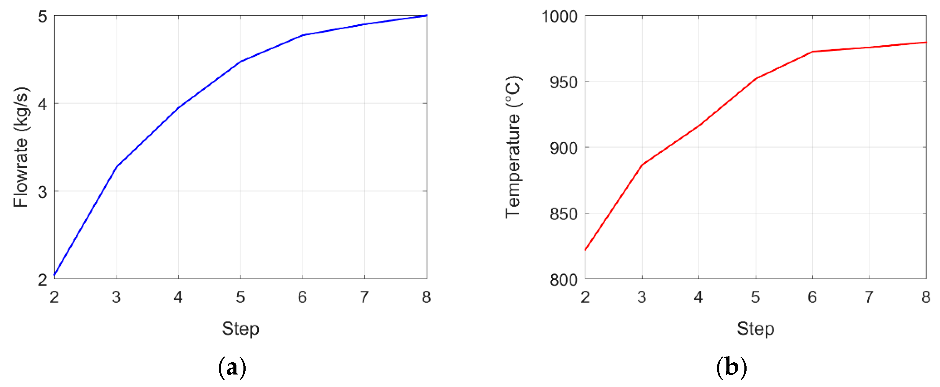
In order to keep a constant particle outlet temperature while increasing the incident power, it is possible to reduce the particle flowrate. As an example, Figure 25 shows the particle flowrate as well as the maximum wall temperature for a particle outlet temperature of 675 °C. The plots start at step 2 because the power at step 1 is too low to reach 675 °C.
5. Discussion
The values of thermal efficiency presented in this paper do not correspond to the upper limit of this technology. Indeed, it is low due to the layout of the existing heliostat field of Themis and of the tower design that constrains the receiver geometry. A more central heliostat field or a more vertical (instead of tilted) tower cladding would lead to higher optical efficiency when applying the aiming point strategy. Upscaling this receiver technology with an adapted heliostat field layout leads to thermal efficiency above 80% [16]. In a commercial power plant, the objective would be to reach a particle temperature as high as possible (~750 °C), which could be achieved by increasing the tubes’ height. In this study, the purpose is to reach high particle temperature for a given 3-m tube height, with the limiting factor being the maximum wall temperature.
Improvements of the heat transfer coefficient between the tube wall and the particles will help reach the higher particle outlet temperature, and hence higher thermal efficiency, while maintaining the maximum tube temperature below 1000 °C.
6. Conclusions
This paper studies the influence of the aiming point strategy on a fluidized particle-CSP prototype. At nominal conditions, the receiver thermal efficiency benefits from the aiming point strategy, increasing at noon from 50.2% up to 52.2%. However, the optical efficiency (including spillage) is strongly affected by the APS, dropping at noon from 83.7% down to 73.7%. Indeed, the inherent spillage loss due to the aiming point strategy leads to a lower optical efficiency and, with a similar thermal efficiency, the lower power available on the tubes results in a lower particle outlet temperature.
The shape of the flux distribution has a strong influence on the wall temperature, particle outlet temperature, thermal and optical efficiency. A tradeoff has to be applied in order to increase the particle outlet temperature as much as possible while keeping the maximum wall temperature below the acceptable limit imposed by the tube material, hence preserving the lifetime of the solar receiver.
The model presented in this paper will be compared with experimental results. A scanning bar travelling at the aperture of the receiver will allow comparison of the simulated and experimental flux distributions with the aiming point strategy. Uncertainties with the optical simulations can be due to the actual tracking error and beam quality of the heliostats. As for the thermal model, it will be confronted to temperature profiles measured with thermocouple data and a thermographic camera installed on a drone.
Future studies should include thermo-mechanical stresses on the tubes, accounting for the flux variations on the receiver during the day, the start-up and shut-down, the thermal shock due to cloud appearance and other fluctuating parameters all along the year such as the DNI or the ambient temperature.
Author Contributions
Methodology, B.G.; software, B.G.; supervision, G.F.; writing—original draft, B.G.; writing—review and editing, G.F. All authors have read and agreed to the published version of the manuscript.
Funding
This project has received funding from the European Union’s Horizon 2020 research and innovation program under grant agreement No 727762, project acronym NEXT-CSP. This work was also supported by the French “Investments for the future” program managed by the National Agency for Research, under contract ANR-10-EQPX-49-SOCRATE (Equipex SOCRATE) and under contract ANR-10-LABX-22-01 (labex SOLSTICE).
Conflicts of Interest
The authors declare no conflict of interest.
References
- Liao, Z.; Li, X.; Xu, C.; Chang, C.; Wang, Z. Allowable flux density on a solar central receiver. Renew. Energy 2014, 62, 747–753. [Google Scholar] [CrossRef]
- Lata, J.M.; Rodríguez, M.; Álvarez de Lara, M. High flux central receivers of molten salts for the new generation of commercial stand-alone. J. Sol. Energy Eng. 2008, 130, 021002. [Google Scholar] [CrossRef]
- Grobler, A. A review of aiming strategies for central receiver. In Proceedings of the 2nd Southern African Solar Energy Conference, Port Elizabeth, South Africa, 27–29 January 2014. [Google Scholar]
- Kelly, B.D. Advanced Thermal Storage for Central Receivers with Supercritical Coolants; Tech. Rep.; Abengoa Solar Inc.: Lakewood, CO, USA, 2010. Available online: http://www.osti.gov/scitech/biblio/981926 (accessed on 30 March 2020).
- Augsburger, G. Thermo-Economic Optimisation of Large Solar Tower Power Plants. Ph.D. Thesis, École Polytechnique Fédérale de Lausanne, Lausanne, Switzerland, 2013. [Google Scholar]
- García-Martín, F.; Berenguel, M.; Valverde, A.; Camacho, E. Heuristic knowledge-based heliostat field control for the optimization of the temperature distribution in a volumetric receiver. Sol. Energy 1999, 66, 355–369. [Google Scholar] [CrossRef]
- Salomé, A.; Chhel, F.; Flamant, G.; Ferrière, A.; Thiery, F. Control of the flux distribution on a solar tower receiver using an optimized aiming point strategy: Application to THEMIS solar tower. Sol. Energy 2013, 94, 352–366. [Google Scholar] [CrossRef]
- Schwarzbözl, P.; Pitz-Paal, R.; Schmitz, M. Visual HFLCA—A Software Tool for Layout and Optimisation of Heliostat Fields. In Proceedings of the 15th SolarPACES Conference, Berlin, Germany, 15–18 September 2009. [Google Scholar]
- Besarati, S.M.; Goswami, D.Y.; Stefanakos, E.K. Optimal heliostat aiming strategy for uniform distribution of heat flux on the receiver of a solar power tower plant. Energy Convers. Manag. 2014, 84, 234–243. [Google Scholar] [CrossRef]
- Dorigo, M.; Gambardella, L. Ant colony system: A cooperative learning approach to the travelling salesman problem. Evol. Comput. 1997, 1, 53–66. [Google Scholar] [CrossRef] [Green Version]
- Belhomme, B.; Pitz-Paal, R.; Schwarzbözl, P.; Ulmer, S. A New Fast Ray Tracing Tool for High-Precision Simulation of Heliostat Fields. J. Sol. Energy Eng. 2009, 131, 031002. [Google Scholar] [CrossRef]
- Collado, F.J.; Guallar, J. A two-parameter aiming strategy to reduce and flatten the flux map in solar power tower plants. Sol. Energy 2019, 188, 185–189. [Google Scholar] [CrossRef]
- Pérez López, I.; Benoit, H.; Gauthier, D.; Sans, J.L.; Guillot, E.; Mazza, G.; Flamant, G. On-sun operation of a 150 kWth pilot solar receiver using dense particle suspension as heat transfer fluid. Sol. Energy 2016, 137, 463–476. [Google Scholar] [CrossRef]
- Kang, Q.; Flamant, G.; Dewil, R.; Baeyens, J.; Zhang, H.L.; Deng, Y.M. Particles in a circulation loop for solar energy capture and storage. Particuology 2019, 43, 149–156. [Google Scholar] [CrossRef]
- Collado, F.J.; Gómez, A.; Turégano, J.A. An analytic function for the flux density due to sunlight reflected from a heliostat. Sol. Energy 1986, 37, 215–234. [Google Scholar] [CrossRef]
- Gueguen, R.; Grange, B.; Bataille, F.; Mer, S.; Flamant, G. Shaping high efficiency, high temperature cavity tubular solar central receivers. Energies 2020, 13, 4803. [Google Scholar] [CrossRef]
- PROMES-CNRS, MESO-STAR SAS. SOLSTICE, SOLar Simulation Tool in ConcEntrating Optics, Version 0.7.1, France. Available online: https://www.labex-solstice.fr/solstice-software/ (accessed on 3 February 2021).
- Caliot, C.; Benoit, H.; Guillot Sans, J.-L.; Ferrière, A.; Flamant, G.; Coustet, C.; Piaud, B. Validation of a Monte Carlo integral formulation applied to solar facility simulations and use of sensitivities. J. Sol. Energy Eng. 2015, 137, 021019. [Google Scholar] [CrossRef] [Green Version]
- Grange, B.; Ferrière, A.; Bellard, D.; Vrinat, M.; Couturier, R.; Pra, F.; Fan, Y. Thermal performances of a high temperature solar absorber based on compact heat exchange technology. J. Sol. Energy Eng. 2011, 133, 031004. [Google Scholar] [CrossRef]
- Benoit, H.; Pérez López, I.; Gauthier, D.; Sans, J.L.; Flamant, G. On-sun demonstration of a 750 °C heat transfer fluid for concentrating solar systems: Dense particle suspension in tube. Sol. Energy 2015, 118, 622–633. [Google Scholar] [CrossRef]
- Le Gal, A.; Grange, B.; Tessonneaud, M.; Perez, A.; Escape, C.; Sans, J.L.; Flamant, G. Thermal analysis of fluidized particle flows in a finned tube solar receiver. Sol. Energy 2019, 191, 19–33. [Google Scholar] [CrossRef]
- Incropera, F.P.; Dewitt, D.P.; Bergman, T.L.; Lavine, A.S. Fundamentals of Heat and Mass Transfer, 6th ed.; John Wiley & Sons: Hokoben, NJ, USA, 2006; pp. 669–722. [Google Scholar]
- Ho, C.K.; Mahoney, A.R.; Ambrosini, A.; Bencomo, M.; Hall, A.; Lambert, T.N. Characterization of Pyromark 2500 paint for high-temperature solar receivers. J. Sol. Energy Eng. 2014, 136, 014502. [Google Scholar] [CrossRef]
- Refractaris, R. Properties of Scuttherm. Available online: www.refractaris.com (accessed on 3 February 2021).
Figure 1.
Side view of panel with the optimized flux profile [3].
Figure 1.
Side view of panel with the optimized flux profile [3].

Figure 2.
(a) Hybrid solar gas turbine concept with particle receiver (particles in solid lines, air in dotted lines)—(b) particle receiver with 40 vertical tubes (tube 1 = left, tube 40 = right).
Figure 2.
(a) Hybrid solar gas turbine concept with particle receiver (particles in solid lines, air in dotted lines)—(b) particle receiver with 40 vertical tubes (tube 1 = left, tube 40 = right).

Figure 3.
Themis site with the tower and 107 heliostats (~5780 m2 of reflective surface).

Figure 4.
A 5 × 5 grid of aiming points.

Figure 5.
Typical objective normalized flux distribution when the Aiming Point Strategy (APS) is applied on the target located at the mid-plane of the tubes and schematic view of the receiver tubes (vertical lines).
Figure 5.
Typical objective normalized flux distribution when the Aiming Point Strategy (APS) is applied on the target located at the mid-plane of the tubes and schematic view of the receiver tubes (vertical lines).

Figure 6.
Discretization of the cavity (unfolded view of the cavity).

Figure 7.
(a) Results of ray-tracing software SOLTICE without APS—interface with ParaView (colors correspond to flux densities, in W/m2)—(b) cosine efficiency of the solar field.
Figure 7.
(a) Results of ray-tracing software SOLTICE without APS—interface with ParaView (colors correspond to flux densities, in W/m2)—(b) cosine efficiency of the solar field.

Figure 8.
Calculated (a) front of tube, (b) back of tube and (c) particle temperature without APS (the results are not acceptable for operating the receiver).
Figure 8.
Calculated (a) front of tube, (b) back of tube and (c) particle temperature without APS (the results are not acceptable for operating the receiver).

Figure 9.
Results of ray-tracing software SOLTICE with APS—Interface with ParaView (colors corresponds to flux densities, in W/m2)—Visualization of the spillage on the tower cladding.
Figure 9.
Results of ray-tracing software SOLTICE with APS—Interface with ParaView (colors corresponds to flux densities, in W/m2)—Visualization of the spillage on the tower cladding.

Figure 10.
Operating heliostats in green—Removed heliostats in red.

Figure 11.
Influence of the spillage loss threshold on the optical efficiency and particle outlet temperature uniformity.
Figure 11.
Influence of the spillage loss threshold on the optical efficiency and particle outlet temperature uniformity.

Figure 12.
Aiming points’ attribution for each heliostat by color-coding. The heliostat color corresponds to the range of aiming points color.
Figure 12.
Aiming points’ attribution for each heliostat by color-coding. The heliostat color corresponds to the range of aiming points color.

Figure 13.
Evolution of the particle temperature deviation and maximum tube temperature during the day for hourly and daily APS.
Figure 13.
Evolution of the particle temperature deviation and maximum tube temperature during the day for hourly and daily APS.

Figure 14.
Influence of horizontal flux distribution profile on the particle temperature at different tube heights—(a) σ2 = 10, (b) σ2 = 12 and (c) σ2 = 14—Simulations at noon.
Figure 14.
Influence of horizontal flux distribution profile on the particle temperature at different tube heights—(a) σ2 = 10, (b) σ2 = 12 and (c) σ2 = 14—Simulations at noon.

Figure 15.
(a) Radial discretization of the tubes—(b) Effect of the solar radiation diffuse reflection on the refractive cavity on the side tubes’ radial flux density profile—Simulation at noon.
Figure 15.
(a) Radial discretization of the tubes—(b) Effect of the solar radiation diffuse reflection on the refractive cavity on the side tubes’ radial flux density profile—Simulation at noon.

Figure 16.
Vertical flux density profiles for tube #20 with polar angle (cf. Figure 15a) as the parameter (in degrees)—Simulation at noon.
Figure 16.
Vertical flux density profiles for tube #20 with polar angle (cf. Figure 15a) as the parameter (in degrees)—Simulation at noon.

Figure 17.
Influence of vertical flux distribution profile on the front tube temperature—(a) b = 0.1, (b) b = 0.5 and (c) b = 1.5.
Figure 17.
Influence of vertical flux distribution profile on the front tube temperature—(a) b = 0.1, (b) b = 0.5 and (c) b = 1.5.

Figure 18.
Influence of peak flux location on the front tube temperature—Peak flux density xpeak at (a) 1.2 m, (b) 1.5 m and (c) 1.8 m from the bottom of the tubes.
Figure 18.
Influence of peak flux location on the front tube temperature—Peak flux density xpeak at (a) 1.2 m, (b) 1.5 m and (c) 1.8 m from the bottom of the tubes.

Figure 19.
Influence of APS on the incident power and maximum flux density—Spillage threshold of 30%.
Figure 19.
Influence of APS on the incident power and maximum flux density—Spillage threshold of 30%.

Figure 20.
Optical (filled contour) and thermal (dotted isolines) efficiency as a function of the peak flux location (parameter xpeak) and the shape of the vertical flux profile (parameter b).
Figure 20.
Optical (filled contour) and thermal (dotted isolines) efficiency as a function of the peak flux location (parameter xpeak) and the shape of the vertical flux profile (parameter b).

Figure 21.
Collection efficiency as a function of the peak flux location (parameter xpeak) and the shape of the vertical flux profile (parameter b).
Figure 21.
Collection efficiency as a function of the peak flux location (parameter xpeak) and the shape of the vertical flux profile (parameter b).

Figure 22.
Particle outlet temperature (filled contour) and maximum tube temperature (dotted isolines) as a function of the peak flux location (parameter xpeak) and the shape of the vertical flux profile (parameter b).
Figure 22.
Particle outlet temperature (filled contour) and maximum tube temperature (dotted isolines) as a function of the peak flux location (parameter xpeak) and the shape of the vertical flux profile (parameter b).

Figure 23.
Number of heliostats added per step.

Figure 24.
(a) Total power on tubes (b) Min/Mean/Max Power per tube (c) Min/Mean/Max maximum flux density per tube (d) Mean particle outlet and wall temperature while increasing the power on the Next-commercial solar power (CSP) receiver.
Figure 24.
(a) Total power on tubes (b) Min/Mean/Max Power per tube (c) Min/Mean/Max maximum flux density per tube (d) Mean particle outlet and wall temperature while increasing the power on the Next-commercial solar power (CSP) receiver.

Figure 25.
(a) Flowrate and (b) Maximum wall temperature while increasing the power on the Next-CSP receiver and keeping a particle outlet temperature of 675 °C.
Figure 25.
(a) Flowrate and (b) Maximum wall temperature while increasing the power on the Next-CSP receiver and keeping a particle outlet temperature of 675 °C.


Table 1.
Optical properties of Pyromark 2500 and ALSIFLEX® 1260.
| Optical Property | Pyromark 2500 | ALSIFLEX® |
|---|---|---|
| Solar Absorptance αS (-) | 0.9 | 0.2 |
| Emissivity ε (-)/IR Absorptance αIR (-) | 0.85 | 0.93 |
Table 2.
Influence of the spillage loss threshold on the APS performance.
| Iteration | Cost Function | Spillage Loss | ||||||
|---|---|---|---|---|---|---|---|---|
| 15% | 20% | 25% | 30% | 15% | 20% | 25% | 30% | |
| 1 | 0.3906 | 0.3906 | 0.3906 | 0.3906 | 0% | 0% | 0% | 0% |
| 100 | 0.2467 | 0.2402 | 0.2447 | 0.2061 | 14.83% | 14.21% | 14.36% | 16.3% |
| 500 | 0.2267 | 0.1529 | 0.0717 | 0.0594 | 14.98% | 19.98% | 24.59% | 26.08% |
| 1000 | 0.2234 | 0.1188 | 0.0646 | 0.0546 | 14.98% | 19.95% | 24.91% | 26.58% |
| 2000 | 0.2214 | 0.1123 | 0.0573 | 0.0504 | 15% | 19.99% | 24.92% | 26.23% |
Table 3.
Evolution of cost function and spillage loss with and without aiming points attribution (AP attribution).
Table 3.
Evolution of cost function and spillage loss with and without aiming points attribution (AP attribution).
| Iteration | Cost Function | Spillage Loss | ||
|---|---|---|---|---|
| AP Attribution | No AP Attribution | AP Attribution | No AP Attribution | |
| 1 | 0.3906 | 0.3906 | 0% | 0% |
| 100 | 0.2061 | 0.2143 | 16.3% | 20.72% |
| 500 | 0.0594 | 0.057 | 26.08% | 28.73% |
| 1000 | 0.0546 | 0.0509 | 26.58% | 29.39% |
| 2000 | 0.0504 | 0.0456 | 26.23% | 29.99% |
Table 4.
Evolution of cost function and spillage loss for hourly and daily APS.
| Iteration | Cost Function | Spillage Loss | ||||||
|---|---|---|---|---|---|---|---|---|
| 8 a.m. | 10 a.m. | Noon | Daily | 8 a.m. | 10 a.m. | Noon | Daily | |
| 1 | 0.3228 | 0.3813 | 0.3906 | 0.3672 | 0% | 0% | 0% | 0% |
| 100 | 0.1942 | 0.2394 | 0.2061 | 0.2073 | 14.94% | 16.4% | 16.3% | 16.99% |
| 500 | 0.0665 | 0.0632 | 0.0594 | 0.0632 | 26.14% | 26.83% | 26.08% | 25.4% |
| 1000 | 0.0596 | 0.0565 | 0.0546 | 0.0584 | 26.89% | 26.25% | 26.58% | 25.69% |
| 2000 | 0.0559 | 0.0546 | 0.0504 | 0.0545 | 27.5% | 25.95% | 26.23% | 25.52% |
Table 5.
Particle temperature deviation and maximum tube temperature for different horizontal distributions.
Table 5.
Particle temperature deviation and maximum tube temperature for different horizontal distributions.
| Horizontal Standard Deviation | Temperature Deviation (°C) | Max Tube Temperature (°C) |
|---|---|---|
| σ2 = 10 | 9.74 | 982 |
| σ2 = 12 | 9.03 | 976 |
| σ2 = 14 | 17.8 | 983 |
Publisher’s Note: MDPI stays neutral with regard to jurisdictional claims in published maps and institutional affiliations. |
© 2021 by the authors. Licensee MDPI, Basel, Switzerland. This article is an open access article distributed under the terms and conditions of the Creative Commons Attribution (CC BY) license (https://creativecommons.org/licenses/by/4.0/).
Share and Cite
MDPI and ACS Style
Grange, B.; Flamant, G. Aiming Strategy on a Prototype-Scale Solar Receiver: Coupling of Tabu Search, Ray-Tracing and Thermal Models. Sustainability 2021, 13, 3920. https://0-doi-org.brum.beds.ac.uk/10.3390/su13073920
AMA Style
Grange B, Flamant G. Aiming Strategy on a Prototype-Scale Solar Receiver: Coupling of Tabu Search, Ray-Tracing and Thermal Models. Sustainability. 2021; 13(7):3920. https://0-doi-org.brum.beds.ac.uk/10.3390/su13073920
Chicago/Turabian StyleGrange, Benjamin, and Gilles Flamant. 2021. "Aiming Strategy on a Prototype-Scale Solar Receiver: Coupling of Tabu Search, Ray-Tracing and Thermal Models" Sustainability 13, no. 7: 3920. https://0-doi-org.brum.beds.ac.uk/10.3390/su13073920
Note that from the first issue of 2016, this journal uses article numbers instead of page numbers. See further details here.